PHYSICAL REVIEW E 70, 026202 (2004)
Spatiotemporal structures in a model with delay and diffusion M. Bestehorn* Department of Theoretical Physics II, Brandenburg University of Technology, 03013 Cottbus, Germany
E. V. Grigorieva† Department of Physics, Belarus State University, 220050 Minsk, Belarus
S. A. Kaschenko‡ Department of Mathematics, Yaroslavl State University, 150000 Yaroslavl, Russia (Received 20 February 2003; revised manuscript received 25 November 2003; published 9 August 2004) Pattern formation described by differential-difference equations with diffusion is investigated. It is shown that an arbitrarily small diffusion induces space-time turbulence just at the instability threshold of the homogeneous stationary solution. We prove this property by deriving a complex Ginzburg-Landau equation on the basis of normal form analysis. Well above threshold, such turbulent structures give way to synchronized states ordered by spirals and targets. This secondary instability can be understood with an asymptotic method representing the system as a cellular automaton network. DOI: 10.1103/PhysRevE.70.026202
PACS number(s): 89.75.Kd, 02.30.Ks, 45.70.Qj, 87.23.Cc
I. INTRODUCTION
Various structures despite their different natures often demonstrate similar features. That implies the existence of some universal laws which are still far from being completely understood. To this end, investigations of a number of basic models have aroused permanent interest, for instance, two-component reaction-diffusion equations or the complex Ginzburg-Landau equation used commonly to simulate such spectacular patterns as spirals, targets, and spatiotemporal chaos in both living and artificial media [1,2]. In most cases, except for models of front propagation, systems of no fewer than two variables are necessary because they can provide excitable or oscillatory behavior of local subsystems so that the physical background of the process is a competition between two players (activator-inhibitor, predator-prey, phaseamplitude, etc.) having different relaxation rates and diffusion scales. There is also another mechanism that can support oscillations in a single-component system. We refer here to the mathematical model proposed by Hutchinson [3] many years ago, ˙ = M关1 − N共t − 兲兴N, N
共1.1兲
which includes a time-delayed term in order to describe the feedback regulation of a biological population living in a homogeneous environment. Here N共t兲 ⬎ 0 is the normalized number of the population, M ⬎ 0 is the Malthusian coefficient of linear growth, and ⬎ 0 means the average age of the species reproducers. In the limit = 0, Eq. (1.1) tells us about one of the simplest quadratic nonlinear laws—the logistic law—of growth with a final stationary state of the
*Electronic address:
[email protected] † ‡
Electronic address:
[email protected] Electronic address:
[email protected]
1539-3755/2004/70(2)/026202(12)/$22.50
population. It is a delay that induces self-oscillations in the absence of interaction with another species or component [4]. Moreover, by varying the only parameter M one can further observe the transition to oscillations of relaxational type [5] in an infinite-dimensional phase space of this functional equation. Equation (1.1) can be exploited for systems with restored resources; hence it is indeed of a general meaning. Related problems arise, in particular, in the dynamics of nuclear reactors [6] or in the dynamics of loss-modulated lasers with optoelectronic feedback [7]. The oscillatory property of the delayed system can also be used to construct neuron models [8]. In a similar way, the delay due to the finite speed of amplifiers has recently been incorporated into a model of an electronic neural network [9]. In order to describe the dynamics of a mobile population living in the area ⍀ 苸 R2, Eq. (1.1) has been generalized to the parabolic boundary value problem [6,10]
冏 冏
N N = D⌬N + M关1 − aN共t − 兲兴N, t
= 0, 共1.2兲 x苸⌫
where ⌬ is the Laplacian, is the normal to the smooth boundary ⌫ of the area ⍀ 苸 R2, and D ⬎ 0 is the mobility coefficient. The Malthusian factor M = M共x兲 ⬎ 0 and the inhomogeneous resistance of the environment a = a共x兲 can be space dependent; if not, they can be set M = 1 , a = 1 without loss of generality. More complicated models of several equations for competing stage-structured population dynamics are discussed in [11]. While the pointlike system (1.1) or the diffusion system (1.2) with = 0 demonstrates rather regular or stationary dynamics, the joint efforts of diffusion and delay in Eq. (1.2) can induce various nonstationary patterns, including spatiotemporal chaos, target centers, and spiral waves. To our knowledge, such a rich variety of structures in single-species systems has not been yet demonstrated; see, for example, the
70 026202-1
©2004 The American Physical Society
PHYSICAL REVIEW E 70, 026202 (2004)
BESTEHORN, GRIGORIEVA, AND KASCHENKO
reviews [1,2,12,13]. This phenomenon seems to be close to that in an optical resonator with passive Kerr-like nonlinear media where two-dimensional feedback provides a spatial transformation of patterns and, as a consequence, nonlocal coupling between distant points [14]. But the differences are essential [15]: (i) contrary to the spatial shift, the time delay introduces extra (infinite) numbers of degrees of freedom and (ii) quadratic nonlinearity leads to relaxation oscillations, which result in more possibilities for the system (1.2). We also note several schemes for time-delayed feedback control of spatial patterns recently proposed and aimed at stabilizing or manipulating patterns originally produced by systems without feedback [16,17]. However, in the case of local feedback one can suppose additional complexity induced by the delayed coupling for every spatial element. Thus pattern formation due to delay and diffusion is certainly of importance. It is hence reasonable to consider systematically such a mechanism in the framework of the fundamental Eq. (1.2) distributed in time and in space and containing only two parameters D and . The paper is organized as follows. In the first part, we use bifurcation analysis and derive the normal form in the neighborhood of the instability threshold of the homogeneous stationary solution N = a−1 of Eq. (1.2). It appears to be the complex Ginzburg-Landau equation with parameters always satisfying Benjamin-Feir instability. That explains the existence of “diffusion chaos” already at threshold. This behavior is replaced by a regime of another sort, namely, spiral waves, when the time delay increases further. These patterns, however, cannot be described completely in the framework of the local analysis. In this case we develop a special asymptotic theory. Instead of boundary value problem systems, we study a set of coupled difference-differential equations which are obtained from Eq. (1.2) as a result of the standard approximation of the Laplacian. The main assumption is that the delay is sufficiently large and the diffusion parameter D is sufficiently small (or the area ⍀ is sufficiently wide, which is biologically natural). These conditions can provide intensive oscillations of spiking type. We first approximate analytically such a solution to the equation without diffusion. Second, we consider the dynamical regimes of two Hutchinson oscillators with diffusionlike coupling. In-phase or out-of-phase oscillations are found depending on the diffusion value, and analytical approximations are obtained of antiphase regimes. Then the dynamics of a one-dimensional open chain as well as that of a circuit of a few coupled oscillators will be studied and the existence of wavelike regimes will be demonstrated. These results have an independent meaning in the context of intensively studied problems on synchronization of relaxation oscillations [18]. Finally, we consider a twodimensional cellular network for which we formulate a simple algorithm for the action on the base of the obtained features of coupled oscillators. This way of investigation, started by Wiener and Rosenblueth [19], enables us to expose the existence of various attractors similar to target centers, spiral waves, etc. II. NORMAL FORM ANALYSIS
First we consider a one-dimensional homogeneous environment. Taking without loss of generality the rate M = 1 , a
= 1 and fixing the size of the system L, we can write Eq. (1.2) as
N 2 = N共x,t兲 − N共x,t兲N共x,t − 兲 + ␦xx N共x,t兲, t
冏 冏 N x
= 0, x=0
冏 冏 N x
共2.1兲 = 0, x=2
where ␦ = L−2D is the diffusion coefficient. In the pointlike system without diffusion, ␦ = 0, a stable limit cycle is created in the vicinity of a certain critical value for the time delay. This result has been obtained by several methods [4] including a normal form analysis. Below we expand the method to the case of the spatially distributed system (2.1) and derive the amplitude equation that predicts one of the well-known ways to obtain complex behavior when ␦ → 0. Note that the diffusion coefficient ␦ = L−2D becomes smaller and smaller when the spatial size of the system increases, so the situation is typical. An analogous situation can occur in systems with a large delay, for which an amplitude equation of a similar universal type has been obtained recently in [20]. The system (2.1) has two stationary homogeneous solutions N共x , t兲 = Nsj, Ns1 = 0,
共2.2兲
Ns2 = 1.
In order to verify their stability we write the equation for a small deviation from the stationary state z共x , t兲 = N共x , t兲 − Nsj, neglect the nonlinear term, and seek for the solution in the form z = exp共t兲共cos kx兲. That results in the characteristic equation = 1 − Nsj − Nsje− − ␦k2 ,
共2.3兲
from which we conclude that the homogeneous solution Ns1 = 0 is always unstable for any perturbation of the wave number k ⬍ ␦−1/2, while the state Ns2 = 1 can be stable or undergoes a Hopf bifurcation at the critical value for the time delay. In the last case, substituting the characteristic roots in the form k = i0 + ␦1k into Eq. (2.3), we find that oscillatory instability with the frequency 0 = 1 occurs for the homogeneous mode k = 0 at the time delay 0 = / 2, and other modes become unstable at ⬎ 0. However, if ␦ → 0 then an (asymptotically) infinite number of spatial modes around the homogeneous one occur in the same critical conditions in a small neighborhood of the critical parameter,
= 0 + ␦1 .
共2.4兲
In this vicinity the modes are excited simultaneously with the same (asymptotic) frequency 0. Following the normal form theory we represent the solution in the form 2
z共x,t兲 = ␦ e 1/2
i0t
+␦
u2je 兺 j=0
2
ij0t
+␦
3/2
u3jeij t + ¯ + c.c. 兺 j=0 0
共2.5兲 where the amplitudes , ukj are functions of the slow time variable ␦t and of the spatial variable x. In addition, each function should obey the corresponding boundary conditions.
026202-2
PHYSICAL REVIEW E 70, 026202 (2004)
SPATIOTEMPORAL STRUCTURES IN A MODEL WITH…
The amplitude of the main term of this series is determined by the following order parameter equation:
冉 冊 冏 冏
s = 1 1 − i
x
2 + 共1 + ic1兲xx − 兩兩2共1 + ic2兲, 2
冏 冏 x
= 0,
x=0
共2.6兲 = 0, x=2
where c1 = −
, 2
c2 =
3 + /2 . 3/2 − 1
共2.7兲
Details of the derivation are given in Appendix A. Equation (2.6) is the complex Ginzburg-Landau equation (CGLE), the universal equation without delay and without any small parameter. Instead, the complex coefficients support both amplitude and phase diffusion. If 1 ⬎ 0, i.e., the time delay exceeds the threshold value / 2, Eq. (2.6) has the homogeneous periodic solution = 0exp共i1␦t兲 where
20 =
51 , 3/2 − 1
1 = −
1/2 + 20共3 + /2兲/5 . 1 + /22
The corresponding homogeneous solution of the original equation is N共x,t兲 = 1 + 2␦1/20 cos 共t + ␦1t兲 + O共␦兲.
共2.8兲
This periodic state can be unstable as the coefficients satisfy the well-known Benjamin-Feir condition [21] 1 + c 1c 2 ⬍ 0 which is satisfied for the coefficients given in Eq. (2.7). Hence we conclude that there is a possibility of diffusion chaos already at onset. The results are the same for a two-dimensional space region with corresponding boundary conditions. Figures 1(a)–1(f) represent numerical simulations of both Eqs. (2.1) and (2.6). For both systems we used a FTCS method for time and space discretization [22]. A mesh of 256⫻ 256 points in space gives a reasonable resolution and accuracy. The code was implemented on an alpha workstation. To compute the delay term in the original system, all former time steps up to the delay time have to be stored in an array, making the code rather memory consuming. This is of course not necessary in the case of the Ginzburg-Landau equation. For both (and also for all following) series, the initial pattern was constructed of two spatially separated squares where the values of the fields were chosen randomly with an equal distribution between ±0.05. For the rest of the layer we put (or N) to zero. Both series clearly show the occurrence of diffusion chaos or phase turbulence. The initial seeds invade the regions without excitation and finally fill the whole domain. Pattern formation stays time dependent and chaotic in the long time limit. When the time delay is increased further, diffusion chaos is replaced by a regime of another sort, namely, spiral waves [Figs. 2(a)–2(c)]. In the original system, turning spirals are
FIG. 1. Numerical solution of (a)–(c) the two-dimensional (2D) Hutchinson equation with diffusion (2.1) and (d)–(f) of the cubic 2D Ginzburg-Landau Eq. (2.6) on a quadratic domain. The initially randomly excited squares expand and finally fill the whole layer. The Benjamin-Feir condition is satisfied and spatiotemporal chaotic patterns are found in the long time limit. = 1.1 0. Here and in all following boxes the side length is scaled to 1, and the small expansion parameter is ␦ = 6 ⫻ 10−6.
formed rather soon and also fill the whole layer at the end. If two fronts meet, they annihilate each other, a behavior well known from excitable media (see, e.g., [12]). However, the spatiotemporal behavior of these patterns cannot be described fully adequately in the framework of a local analysis. Actually, to trace the evolution of the system further away from threshold one can continue the procedure and obtain higher order nonlinear terms. Then the normal partial differential equation takes the form
冉 冊
= 1 1 − i + 共1 + ic1兲⌬ − 兩兩2共1 + ic2兲 + ␦兩兩4共c3 2 s + ic4兲,
共2.9兲
where c3 =
3共7 − 8兲 , 10共3 − 2兲
c4 =
3共2 + 7兲 . 5共3 − 2兲
The real part of the coefficient of the quintic term is positive, c3 ⬎ 0. This means that when the amplitude of the solution becomes relatively large the system leaves the local vicinity of the homogeneous solution and diverges. Nevertheless, bounded solutions of Eq. (2.9) can be found for not too large 1. Figures 2(d)–2(f) show frames where the suppression of diffusion chaos and the tendency to form traveling waves and spirals can be seen. This picture is supported by the fact that the Benjamin-Feir unstable region is bounded from above in the k-1 plane if complex quintic terms are present [23]. To demonstrate this we make for Eq. (2.9) the ansatz
共x,y,t兲 = 关Ak + a共x,t兲兴exp兵i关kx + 共k兲t + ⌽共x,y,t兲兴其 共2.10兲 with Ak being the smaller (stable) real root of
026202-3
PHYSICAL REVIEW E 70, 026202 (2004)
BESTEHORN, GRIGORIEVA, AND KASCHENKO
FIG. 2. (a)–(c) Numerical solution of the 2D Hutchinson equation with diffusion (2.1) well above threshold, = 1.5 0. Now spirals are formed early and persist in time. The development strongly resembles that known from excitable media. (d)–(f) Numerical solution of the quintic Ginzburg-Landau Eq. (2.9), but above threshold, 1 = 0.41. The diffusion chaos is suppressed and more regular structures evolve as a secondary instability, already showing the tendency to form spirals. (g)–(i) Numerical solution of the seventh order Ginzburg-Landau equation with global stability. Spirals and excitable behavior are found well above threshold for 1 = 0.8.
1 − k2 − A2k + ␦c3A4k = 0 and
共k兲 = − 1/2 − c1k2 − c2A2k + ␦c4A4k . Note that a = 0 , ⌽ = const is an exact solution of Eq. (2.9) and describes traveling waves. To test their stability, one may perform the usual linear analysis. After adiabatic elimination of the amplitude [21], one arrives at a linear phase diffusion equation having the form 2 t⌽ = vxx⌽ + D储xx ⌽ + D⬜2yy⌽
共2.11兲
with the diffusion coefficients D⬜ = 1 +
− c2 + 2␦c4A2k −1+
D储 = D⬜ +
2␦c3A2k
c1 ,
共2.12兲
.
共2.13兲
2k2 −
A2k
+ 2␦c3A4k
Both coefficients are negative at threshold (Benjamin-Feir instability) but may change their sign for larger values of 1, allowing for a region of stable traveling waves or homoge-
FIG. 3. Phase diagram found by the method of phase equations applied to the quintic CGLE. Bounded solutions exist between the two bold lines. Thin solid line, D⬜ = 0; thin dashed line, D储 = 0 In the small region between the upper bold and the dashed line nonchaotic solutions are possible.
neous oscillations (Fig. 3). It is in this region where spirals can be formed. Finally, Figs. 2(g)–2(j) presents solutions of the CGLE including a seventh order term of the simple form − 兩 兩 6 , which is here not systematically derived from the basic equation, but only used to assure global stability. Now the region of larger 1 can be explored and spirals are clearly the preferred structure. To get a more accurate insight into the mechanisms of spiral dominated structures, we now leave the local approximation in normal forms and wish to present another way to understand pattern formation far away from threshold in the next part. III. DYNAMICS OF COUPLED HUTCHINSON EQUATIONS WITH A LONG TIME DELAY
Here we turn to the systems of coupled differentialdifference equations ˙ = D⌬ N + N关1 − N共t − 1兲兴, N K
共3.1兲
where ⌬K is the difference analogy of the Laplacian, taking into account the boundary conditions and geometry of the region, the current time variable is normalized so that the time delay is equal to unity, and N共t兲 苸 RK is a vector whose elements mean “the population number” in the corresponding subcell of the area ⍀. The system (3.1) may be also referred to as a model describing the dynamics of the population living in k local areas, and the operator D⌬K describes
026202-4
PHYSICAL REVIEW E 70, 026202 (2004)
SPATIOTEMPORAL STRUCTURES IN A MODEL WITH…
the exchange of specimens between neighboring areas in the absence of migrations within the areas. The constant characterizes the time delay, which is assumed to be sufficiently large, Ⰷ 1, while the coupling coefficient D Ⰶ 1. These conditions are not very hard because numerical simulation shows that ⬃ 20 ⬇ 3 is already long enough to induce strongly nonlinear oscillations. Without coupling 共D = 0兲 each equation of the system (3.1) has a slow-oscillating periodic solution N0共t兲. We find such a solution to be stable in a system with the coupling coefficient D exceeding the critical one Dc = exp共−兲. That is why it is convenient to consider the small diffusionlike coefficient in the form D = e −,
⬎ 0;
then the critical coefficient of diffusion corresponds to the critical c = 1. Being simpler than Eq. (1.2), the model (3.1) has nevertheless a rich set of attractors. Below we shall obtain analytical approximations for the most important solutions from this set, namely, the slowly oscillating solution characterizing synchronous oscillations as well as the antiphase solution for two coupled oscillators. We then numerically demonstrate solutions with shifted phases in one-dimensional open and closed chains and in a two-dimensional region. The solutions can be interpreted as wavelike patterns moving with a velocity dependent on the coupling coefficient. When the diffusion coefficient decreases the oscillations become out of phase and the patterns get more and more complicated. Our conclusions, however, have to be considered only as tendencies for the original parabolic Eq. (1.2). It turns out to be impossible to expand correctly the results obtained to the boundary value problem (1.2) because increasing the dimension K of the system (3.1) requires increasing the parameter . Nevertheless, the observed structures correlate quite well with those found for the original model. A. Solitary Hutchinson oscillator
A single Hutchinson oscillator with a large time delay is determined by ˙ = N关1 − N共t − 1兲兴, N
Ⰷ 1.
FIG. 4. (a) Numerical solution of Eq. (3.2) (bottom) and its analytical approximation (top) by Eqs. (B2), (B3), (B7). = 3. (b) Synchronous and (c) antiphase solutions of Eqs. (3.5) with = 4 and = 0.5 (b), 2.7 (c). The vertical axis denotes the number of the population 共N , N0 苸 关0 , 10兴 , N1 , N2 苸 关0 , 30兴兲.
delayed systems, which allow us to integrate the equation step by step using the large parameter . It is possible to show that after a certain time these solutions again fall within S. Thus, the operator of the shifting along the trajectories, which makes a function from S correspond to a function also from S, is naturally determined. To a fixed point of the operator there corresponds a periodic solution of Eq. (3.2) of the same stability. Let us choose t = 0 at the moment of the onset of a spike and determine the set S0 of initial functions 共s兲 , s 苸 关−1 , 0兴, in the form
共3.2兲
From the local analysis we know that there is a stable limit cycle if ⬎ / 2. This cycle is close to a harmonic one at its creation. Far away from threshold the harmonic oscillations are transformed into sharp spikes with large-period pulses. The corresponding periodic solution is called slowly oscillating as the intervals between neighboring local maxima or minima are larger than the time delay. In order to get such a solution analytically we consider the phase space of Eq. (3.2), which is the Banach space C关−1,0兴 of continuous functions, i.e., the values of the functions from C关−1,0兴 should be given as initial conditions. In this space, we shall distinguish a (fairly wide) set S and construct uniform asymptotic approximations of the solutions with initial conditions from this set. One way for the asymptotic buildup of solutions of the spiking type is opened by peculiarities of
S0:共s兲 = es关1 + g共s兲兴;
兩g兩 艋 −2,
g共0兲 = 0. 共3.3兲
Details of the further procedure are given in Appendix B. Finally, we find that Eq. (3.2) has an orbitally stable periodic solution N0共t兲 with the period T0 =
e 关1 + o共1兲兴.
共3.4兲
The maxima and minima of the spikes Nmax = e−1关1 + o共1兲兴, Nmin = exp兵− e关1 + o共1兲兴其 follow each other in a time tmin − tmax = 1 + o共1兲, which determines the width of the spike. The comparison between numerical and analytical solutions given in Fig. 4(a) confirms
026202-5
PHYSICAL REVIEW E 70, 026202 (2004)
BESTEHORN, GRIGORIEVA, AND KASCHENKO
that the approximation obtained is already quite satisfactory for = 3, i.e., twice above the threshold. Summarizing, after generation of a spike of large amplitude ⬃e−1, the system recovers its properties during the long period ⬃e / , which is caused by the fact that the population decreases to a superexponentially small value. From the biological point of view, such a dramatic scenario can result in disappearance of the population. But it can easily be prevented by a small additional influence like migration from neighboring areas. We consider this mechanism in the next section. B. Two coupled Hutchinson oscillators
The dynamics of two coupled Hutchinson oscillators is governed by the system ˙ = N 关1 − N 共t − 1兲兴 + D共N − N 兲, N 1 1 1 2 1 共3.5兲 ˙ = N 关1 − N 共t − 1兲兴 + D共N − N 兲, N 2 2 2 1 2 where the coupling term D共N2 − N1兲 is the difference analogy of the diffusion operator in the original partial differential equation, D = e− , ⬎ 0. If the coupling coefficient is relatively strong, then the system (3.5) demonstrates in-phase oscillations as shown in Fig. 4(b). In this case each equation of the system (3.5) has the slowly oscillating periodic solution N0共t兲 given in the previous section. The synchronous solution becomes unstable when the coupling becomes weaker than the critical one, ⬎ c. Oscillations are still intensive but they are antiphase and their period decreases essentially as Fig. 4(c) demonstrates. In order to prove analytically the existence of such antiphase regimes and estimate the critical value c we consider a sufficiently wide set of initial conditions, namely, N1共s兲 = 共s兲 苸 S1 , N2共s兲 = 共s兲 苸 S2, where S1 = 兵共s兲 苸 C关−1,0兴:0 ⬍ 共s兲 艋 共1 + c兲exp s,
共0兲 = 1其, 共3.6兲 S2 = 兵共s兲 苸 C关−1,0兴:c1exp 共s − 兲 艋 共s兲 艋 c2exp 共s − 兲其, and 0 ⬍ c ⬍ 1 , 0 ⬍ c1 ⬍ 1 , c2 ⬎ 1. Such conditions correspond to the situation in which the first oscillator is ready to generate a spike, N1共0兲 = 1, while the second oscillator is still in a refractory phase as N2共0兲 ⬃ exp共−兲. Integrating Eqs. (3.5) asymptotically for t 苸 关0 , 1兴, one finds N1共t兲 ⬃ exp共t兲 and N2共t兲 ⬃ exp关共t − 兲兴. If ⬍ 1 the spike of the second oscillator starts during the spike of the first one. That causes further synchronization of the oscillators. In the case of ⬎ 1 the spike of the second oscillator can start only after the spike of the first one and antiphase conditions are still valid. Thus the critical coupling is c = 1, which is also confirmed by the numerical integrations. We leave further details of the proof for Appendix C and formulate the result here. Let t1 be the first positive root of the equation N2共t兲 = 1. Then for each c , c1 苸 共0 , 1兲 and c2 艌 , there is a sufficiently large for which
N1共s + t1兲 苸 S2,
N2共s + t1兲 苸 S1,
t1 = + o共1兲. 共3.7兲
That means the initial situation (3.6) arises again in time t1 = + o共1兲 with replacing N1 ↔ N2. From the above statement one may conclude that N1共s + t2兲 苸 S1,
N2共s + t2兲 苸 S2,
t2 = 2 + o共1兲, 共3.8兲
where t2 is the next root of the equation N1共t兲 = 1 following t1. Hence, the solutions again fall within the same set of functions and T = t2 = 2 is a period of spiking antiphase oscillations of the system (3.5). The period T is essentially shorter than the period T0 of the slowly oscillating solution because the minimal values of the population increase from superexponentially to exponentially small values. Numerical simulations readily confirm these conclusions. From the ecological point of view, in both cases of independent areas, D = 0, or of strongly coupled areas, D ⬎ exp共−兲, oscillations of a single species are determined by the function N0共t兲 which are abrupt and can be dangerous for populations to survive and develop. The average number of the population 1 t→⬁ t
M = lim
冕
t
N共s兲ds
0
in the stable periodic regime is M(N0共t兲) = 1. However, in the case of weak coupling, D ⬍ exp共−兲, the average population increases essentially, M(N1共t兲) ⬃ exp共兲 , Ⰷ 1, and living conditions become more safe and predictable. The same result is expected in an isolated area due to an additional small influence of the order of exp共−兲 , ⬎ 1. Thus weak external forcing can be an effective tool for control of population growth. C. Open chain of coupled oscillators
An open chain of coupled Hutchinson oscillators is described by ˙ = D共N − 2N + N 兲 + N 关1 − N 共t − 1兲兴, N k k+1 k k−1 k k 1 艋 k 艋 K,
N 0 ⬅ N 1,
NK+1 ⬅ NK ,
共3.9兲
where D = e− , ⬎ 0 , Ⰷ 1. Analytical estimations of typical dynamical regimes can be obtained on the base of the method applied above. Rather than giving here cumbersome formulas we illustrate our conclusions by numerical simulations in the case of five oscillators 共K = 5兲. Figures 5(a)–5(c) demonstrate three possible spiking regimes: completely synchronized, shifted phase, and antiphase states. In Fig. 5(a) one can see a synchronous solution N0共t兲 which is realized if the coupling coefficient is relatively strong, ⬍ ␣K. Here the constant ␣K ⬍ 1 depends on the total number of oscillators K so that ␣K → 0 under K → ⬁. As mentioned before, oscillations are intensive and their period is asymptotically large, ⬃exp共兲.
026202-6
PHYSICAL REVIEW E 70, 026202 (2004)
SPATIOTEMPORAL STRUCTURES IN A MODEL WITH…
D. Closed chain of coupled oscillators
The dynamical behavior of coupled Hutchinson oscillators organized as a ring is described by the system ˙ = D共N − 2N + N 兲 + N 关1 − N 共t − 1兲兴, N k k+1 k k−1 k k 1 艋 k 艋 K,
FIG. 5. Patterns corresponding to the temporal evolution of intensities of five coupled oscillators calculated with Eqs. (3.9) for (a) K = 5 , = 4 , = 0.3, (b) = 0.8, (c) = 1.6, and (d) Eqs. (3.10) and (3.12) and (e) (3.12), (3.13) for = 0.7. The horizontal axis is the oscillator index 共k = 1 , . . . , 5兲, the vertical axis the time 共t 苸 关0 , 30兴兲. The highest (lowest) intensity is represented by white (black) domains.
Figure 5(b) shows a wave structure formed by oscillations of a shifted phase under ␣K ⬍ ⬍ 1. Spikes of the main oscillator (in our case N3) generate waves of spikes moving to both ends along the chain and creating a structure that is a one-dimensional analog of targets. The period of oscillations Tk is less than T0共兲 but still asymptotically long. Spikes of the k oscillator are retarded with respect to the spike of the leading oscillator k0 in time by 兩k − k0兩. Therefore characterizes the velocity of the wave. The maximal amplitude of the main spike is slightly smaller than the maxima of the spikes on the boundary. The appropriate initial conditions are Nk共s兲 = k共s兲 苸 Sk where Sk = 兵k共s兲 苸 C关−1,0兴:0 ⬍ 共s兲 艋 共1 + ck兲exp 共s − 兩k − k0兩兲其 共3.10兲 and ck ⬃ 1 are arbitrary constants. One can also organize the initial conditions to give “antitargets:” Sk = 兵k共s兲 苸 C关−1,0兴:0 ⬍ 共s兲 艋 共1 + ck兲exp 关s − 共k0 − 1兲 + 兩k − k0兩兴其.
共3.11兲
In this case waves periodically starting from the ends of the chain annihilate in the center. In Fig. 5(c) we present the antiphase solution realized for relatively weak coupling with ⬎ 1. All functions N j having odd indices generate spikes almost at the same time; the duration of the spikes is close to 1. At a time + O共−1/2兲 later the functions of the even numbers begin to grow, etc. The basic characteristics of Nk共t兲 do not depend on k: T = 2 + o共1兲,
Nmax = exp 关1 + o共1兲兴,
Nmin = exp关− c兴,
N 0 ⬅ N K,
NK+1 ⬅ N0 ,
共3.12兲
where D = e− , ⬎ 0 , Ⰷ 1. In such a circuit four qualitatively different regimes are possible. Again, the completely synchronous solution Nk共t兲 = N0共t兲 is observed if the coupling coefficient is relatively strong, ⬍ K where K ⬍ 1 depends on K so that K → 0 under K → ⬁. Targets appear under 2 / K ⬍ ⬍ 1. In contrast to the open chain, in the ring each oscillator can be the central one, for example, N2 has been chosen as the leader for Fig. 5(d). The waves of spikes propagate from this oscillator in both directions and annihilate at the opposite diameter. The regime can be realized if the period of oscillations is sufficiently longer than the round trip time of the wave. In the case 2 / K ⬍ ⬍ bK , bK ⬍ 1, there can also exist attractors of the traveling wave type, as shown in Fig. 5(e). In this case special initial conditions have been prepared in order to force spikes to propagate in a certain direction over the circle, namely, we set Nk共s兲 = k共s兲 苸 Sk where Sk = 兵k共s兲 苸 C关−1,0兴:0 ⬍ k共s兲 艋 共1 + ck兲exp共− 兲,
k ⫽ i其,
共3.13兲 Si = 兵i共s兲 苸 C关−1,0兴:0 ⬍ i共s兲 艋 exp关ci共k0 − i兲共s + 1兲兴, i = k0 − 1,k0,k0 + 1其, and ci ⬎ 1 , ck ⬃ 1 are arbitrary constants. Here, the initial function k0+1 corresponds to the excitory state, the functions k0 , k0−1 provide the refractory state of oscillators, and all other k⫽i correspond to the rest states. Then the wave of excitation moves from k0 to k0 + 1 over the circle, doing the round trip in time TK ⬃ K + o共1兲, which is, hence, the period of oscillations. The neighboring spikes are shifted with respect to each other in time by ⬃. In the case of a long ring circuit (large K) two-, three -, and so on spike traveling solutions are also possible. The existence of such traveling waves in the ring is important for understanding wave structures in a twodimensional network in which an excitation circulated permanently in closed contours can create complicated periodic patterns. In the case of weak coupling, ⬎ 1, the oscillations are analogous to oscillations in an open chain and produce celllike zigzag structures. The spikes of neighboring oscillators follow each other in a time ⬃. If K is odd the structures are rather regular because odd (even) oscillators are synchronized. If K is even, then more complicated patterns can be observed. E. Two-dimensional network
c ⬎ 0.
Such solutions zigzag most over the “spatial” variable k and correspond to a stable cell-like structure.
The conclusions made above on the dynamics of chains can be expanded to the case of a two-dimensional network described by
026202-7
PHYSICAL REVIEW E 70, 026202 (2004)
BESTEHORN, GRIGORIEVA, AND KASCHENKO
˙ = N 关1 − N 共t − 1兲兴 + D N ij ij ij
兺
共m,k兲苸Zi,j
共Nmk − Nij兲, 共3.14兲
where D = e− , ⬎ 0 , Ⰷ 1 , i , j characterize the plane coordinates of the oscillator, and Zi,j is the set of coordinates of the nearest, say, six, cells. In such a network, a spontaneous spike of the Nij oscillator at t = 0 induces spikes of the nearest Zij oscillators at t ⬃ . They initiate, in turn, spikes of all neighboring oscillators excepting, however, Nij, and so on. Thus, a wave of spikes is created and moves to the boundary of the region. The collision of two waves results in their annihilation. That is why the final structures depend essentially on the initial states of the oscillators. The number of attractors is enormous. In the case of 0 ⬍ ⬍ 1, the wave process described may be reproduced by the cellular automaton introduced in the following. In a discretized time T each cell can take discrete states numbered 1 , 2 , . . . , m , 0 where 0 means the rest state in which a cell is ready to respond to an incoming influence by a spike, the state 1 corresponds to the spike of the cell, and the states 2 , . . . , m correspond to the refractory phase when the cell does not respond to an external force. It follows from the previous consideration that the duration of the refractory state m can be estimated from m = 关共t1 + 1兲 / 兴 where 关·兴 means one integer part, and t1 = 1 + o共1兲 is the duration of a spike. The period of delay-induced excitation of a solitary cell is M = 关exp共兲 / 共兲兴. Here Ⰷ 1 is supposed, and hence M Ⰷ m. Once a cell has passed the last state m it waits in the state 0 until the moment when another cell of state 1 appears among the neighbors or 共M − m兲 time steps pass. Then its state changes again as s = 1 , 2 , . . . , m , 0. Such an approach looks rough but it allows us to efficiently simulate pattern formation and to determine the initial conditions leading to different structures. In general, the simple rules given above can be specified, as many authors did, for instance, to take into account dispersion in reactiondiffusion processes [24] or to investigate cooperative phenomena in laser dynamics [25]. We note, in addition, that contrary to many axiomatic models our automaton is reasonably determined and its main quantitative characteristics, the speed of waves and the duration of the refractory state m, have been derived. Excitory, refractory, or rest states of a cell in the system (3.14) can be prepared by choosing the initial functions in the way described in Sec. III D. Hence under large enough we expect a good correspondence between the dynamics of the automata and the network (3.14), although the correspondence to the dynamics of the continuous system (1.2) is not evident. To reproduce structures related to solutions of the parabolic boundary problem (1.2) we take two types of initial conditions. Figure 6 is obtained for automata containing 50 ⫻ 50 cells. In these figures, full points determine excited spike states, s = 1; the duration of the refractory phase is m = 5. The initial conditions have been chosen as a few arbitrarily placed excited oscillators of state s = 1 and pairs of states s = 1 , 2, while all other oscillators are in the rest state
FIG. 6. Creation and evolution of target centers (a), (b) and spirals (c), (d) in the cellular automaton. In the beginning T = 0 (a), (c) all cells are in the rest state s = 0 excepting cells in the excitable state s = 1 (black dots) and refractory cells of state s = 2 (white dots). (b),(d) Further evolution of the wave front at T = 10 is marked by black dots (state s = 1). Period of self-excitation M = 25.
s = 0. One can then observe the creation and evolution of targets of different periods. Figure 7 demonstrates analogous targets to those realized in the diffusion system (1.2) with similar initial conditions. The larger wavelength in Figs. 7(d)–7(f) is mainly determined by the properties of a single oscillator; hence, the period is of the order of ⬃exp共兲, whereas the small period Figs. 7(a)–7(c) is determined by the coupling strength. Let the initial front 共s = 1兲 in the automaton be the line segment that touches the boundary, and similar segments in the refractory state s = 2 are located one step below (above), as shown in Fig. 6(c). All other oscillators are in the state s = 0. When time passes the waves twist around their free ends
FIG. 7. Targets as solution of the partial differential equation (PDE) (2.1) with delay = 0.5. (a)–(c) show short wavelength patterns obtained if the central point is fixed for all time at N = Ns1. Long wavelength patterns (d)–(f) evolve if N = Ns1 only at t = 0 (see text).
026202-8
PHYSICAL REVIEW E 70, 026202 (2004)
SPATIOTEMPORAL STRUCTURES IN A MODEL WITH…
FIG. 9. Memory effect in the cellular automaton. White dots mark the front of the waves (state s = 1). At the initial moment (a) T = 0 some of the excitable points s = 1 are included into the closed contour which consists of r共m + 1兲 cells (r integer), m = 2, in the consecutive states 1 , 2 , 0, and form the image “T.” Period of selfexcitation M = 25. (b) Pattern at T = 5. (c) Finally, at T = 34 a number of spirals and “T” appearing with the period 共m + 1兲 survive.
FIG. 8. One, two, and four-arm spirals from PDE (2.1). The initial conditions are chosen in a similar way as those in Fig. 6(c) (see text).
and evolve into single or double spirals, Fig. 6(d). Figures 8(a)–8(i) represent spirals in the diffusion system (2.1). Here, we used initial conditions similar to those in Fig. 6(c). In Fig. 8(a) the line segment was chosen according to Eqs. (3.13) with N共x0 , y , t兲 = exp共0.6兲 for − 艋 t 艋 0 and 0 艋 y 艋 L / 2, whereas neighbors were put at N共x0 ± ␦x , y , t兲 = exp关⫿共1.5t + 兲兴. As a result, the segment is forced to move in the negative x direction; its free end in the center of the domain twists and forms a (one-armed) spiral. In this way it is also possible to get coexisting reverberators as well as spirals with an arbitrary number of arms using an initial configuration of the form of Fig. 6(c) [see Figs. 8(d)–8(i)]. In the long time limit only the one-armed spiral seems to survive, but the decay time of multiarmed spirals increases essentially with increasing time delay. By synthesizing the initial conditions one can study the evolution of complicated patterns [26]. In particular, the wave circulation along a ring discussed in Sec. III D can create a target without the leading oscillator in the twodimensional network. It is also possible to construct a more complex front, say in the form of the letter “T” as shown in Fig. 9. At the initial moment T = 0, the image was formed by excitable points 共s = 1兲 of a closed contour which consists of r共m + 1兲 cells (r integer), in the consecutive states 1 , 2 , 3 , . . . , m , 0, and we put this contour on a random background. Finally, in Fig. 9(c), a number of spirals and periodically appearing “T” [5] survive. It would be interesting to realize such wave structures in the continuous system (1.2), which we leave for future work. The existence of contours providing circulation of excitation and, as a consequence, periodic attractors of complex form
can be associated with a dynamical image memory. This problem is under intensive permanent investigations [27] and from this point of view we remark that in many aspects the behavior of the Hutchinson oscillator is similar to the behavior of a formal oscillating neuron hence, the system (3.14) can be proposed to model and study coupled neurons. For biological neural networks, however, multidimensional diffusion problems are more natural, as each neuron, is influenced by hundreds or thousands of other neurons and, in turn, controls the same number of neurons. At the same time we note that solutions of traveling wave type can also be observed in systems of globally coupled (all to all) oscillators; in particular, attractors called “splay states” have been obtained in circuits of Josephson junctions [28] or in the dynamics of a multimode solid-state laser [29]. IV. CONCLUSION
We considered pattern formation in a system with diffusion and delay, which can be encountered in many fields such as population dynamics, biology, mechanical engineering, or physics. Due to the interplay of these processes, very complicated structures can arise, such as spiral waves and space-time turbulence. It has been shown previously [13] that steady inhomogeneous regimes in diffusion dominated systems without delay can exist only if the size of the area is sufficiently large and, additionally, is of a complex geometry, in particular, is not convex. In a simple region, multicomponent systems governed by two or more parabolic equations are necessary to observe complex structures in space and time. Thus it is a delay that already induces in a natural way a rich variety of patterns in the single-species diffusion equation. Our work rigorously relates the diffusion chaos already found in a partial differential delay equation, namely, the diffusive Hutchinson equation, at threshold with the wellknown Benjamin-Feir instability in the complex GinzburgLandau equation. It turned out that the complex Ginzburg-Landau equation serves as a normal form valid near the first bifurcation of the Hutchinson equation. To describe patterns well above threshold, higher order terms in the Ginzburg-Landau equation are involved. However, this approach is not really sufficient be-
026202-9
PHYSICAL REVIEW E 70, 026202 (2004)
BESTEHORN, GRIGORIEVA, AND KASCHENKO
cause far from threshold oscillations are transformed into strongly nonlinear spikes, for which the amplitude of the second harmonic of Fourier expansion is of the same order as the first one. Hence the inclusion of nonresonant nonlinear terms that break the symmetry of the phase in the complex Ginzburg-Landau equation might be necessary, as it may turn a stable limit cycle into a spike solution [30,31]. The temporal behavior of 共t兲 obeying
t = 共 + i兲 + a2 − 兩兩2
u33 = − u22
ACKNOWLEDGMENTS
This research has been supported by the INTAS, Grant No. 00-867, and the German Academic Exchange Service, DAAD Grant No. A/03/06768.
− exp共− i00兲 , i20 + exp共− i200兲
exp共− i00兲 + exp共− i200兲 , i30 + exp共− i30兲
* 关exp共− i200兲 + exp共i200兲兴, u40 = − u22u22
共4.1兲
shows spikes for certain values of the parameters a and . If diffusion is added, target patterns and spirals can be found in two spatial dimensions [32]. Another explanation of patterns observed far away from threshold is given by constructing a cellular automaton. The algorithm and quantitive characteristics are based on the analytical investigations of the dynamics of coupled delayed oscillators. Cells can be excited spontaneously or by the influence of other cells and generate spikes. After the spike, the cell recovers its properties during a long refractory period. This behavior is well known from excitable media and can explain the spiral waves of a mobile population living in a homogeneous environment. The obtained analytical estimations also explain the dramatic character of oscillations of an isolated population as it decreases in minima to superexponentially small values. The same is valid for the synchronized regime in coupled populations if the coupling is larger than exp共−兲. In the case of relatively weak coupling, we demonstrate various types of phase synchronization, resulting in the essential growth of the average population and improving living conditions. Phase synchronization also relates to processes of pattern formation. The advantages of the analytical method applied are that we can approximate the speed of waves in the discrete network, the duration of the refractory phase, and initial conditions leading to the development of different structures. In this way it is possible to get on demand various structures like targets, multiarm spirals, or traveling waves in a onecomponent system with local delayed feedback. Similar autowaves arise in chemical multicomponent oscillatory reactions, heart pacemaker cells, laser light generation, oscillatory neural networks, etc. [33–37] Thus, the imitation of complex phenomena in various autowave media is one of the possible fascinating applications of the diffusive Hutchinson oscillator.
u42 = − u33*
exp共i00兲 + exp共− i300兲 . i20 + exp共− i200兲
At the order ␦3/2 we find the equation for the main amplitude : 共1 + 20兲
= 共1 − i0兲⌬ + 1共1 − i0兲 − 兩2关30 − 1 + i共3 ␦t + 0兲兴/5,
冏 冏 x
= 0, x=0
冏 冏 x
= 0. x=1
With the rescaled time variable s = ␦t共1 + 20兲−1 and amplitude
→ „共30 − 1兲/5…1/2 the equation is transformed to the standard form (2.6) of a complex Ginzburg-Landau equation. APPENDIX B
The method of asymptotic integration described below permits one to obtain uniform asymptotic formulas for steady-state regimes with any degree of accuracy, but we restrict ourselves to the leading terms of the solutions. Let us denote the sequential positive time moments when N共t兲 = 1 by t0 , t1 , . . . so that t0 , t2 , . . . , t2k , . . . are moments of the onset of spikes while t1 , t3 , . . . , t2k+1 , . . . are moments of the cessation of spikes. We choose t0 = 0 and the initial conditions from the set S0 given by Eq. (3.3), N共s兲 = 共s兲 , s 苸 关−1 , 0兴. Under these conditions one can integrate Eq. (3.2) and get N共t兲 = exp关t − e共t−1兲兴关1+ o共1兲兴,
t 苸 关0,1兴.
共B1兲
The solution increases up to the maximum Nmax = N共1兲 = e−1关1 + o共1兲兴 at the end of this interval. During the next interval t 苸 关1 , 2兴 the solution decreases monotonically as ˙ ⬍ 0 because N共t − 1兲 Ⰷ 1. Replacing N共t − 1兲 by the function N (B1) and integrating Eq. (3.2) at this interval we find N共t兲 = exp兵t + e关e−e
共t−2兲
−
− e−e 兴关1 + o共1兲兴其,
t 苸 关1,2兴, 共B2兲
from which we estimate the moment
APPENDIX A
Inserting the series (2.4),(2.5) into the equation for deviation z共x , t兲 and collecting terms of the same order ␦ one finds the slowly varying functions uij: u20 = 0,
u22 = *2
t1 = 1 +
冉 冊
ln ln +o
共B3兲
when N共t1兲 = 1. The solution decreases further in accordance with
026202-10
PHYSICAL REVIEW E 70, 026202 (2004)
SPATIOTEMPORAL STRUCTURES IN A MODEL WITH…
N共t兲 = exp兵t − 1 + e关e−e
共t−2兲
˙ +N ˙ 艋 共e− + 兲共N + N 兲. N 1 2 2 1
− 1兴关1 + o共1兲兲兴, (B4)
t 苸 关2,1 + t1兴其,
Taking into account the initial conditions (3.6) one can then estimate
up to the minimum at t = t1 + 1:
N1 艋 关1 + c + o共1兲兴et ,
N共1 + t1兲 = Nmin ⬇ exp关2 + ln − e 兴 ⬇ exp兵− e 关1 + o共1兲兴其. 共B5兲 From this moment the solution increases monotonically as N共t − 1兲 = o共1兲; hence N共t兲 = N共1 + t1兲e
共t−1−T1兲关1+o共1兲兴
= exp共t − − e 兲, (B6)
t 苸 关1 + t1,t2 兴.
N2 艋 N2共0兲et + e共t−兲
e t2 = 关1 + o共1兲兴,
共B7兲
the population again reaches unity, N共t2兲 = 1, and the problem of further constructing the solution is returned to the original problem because N共t2 + s兲 苸 S0 , s 苸 关−1 , 0兴. Finally, let us introduce the operator of the shifting along the trajectories ⌸(共s兲) = (N共t2 + s兲) , s 苸 关−1 , 0兴, and a set S共␣兲 : 共s兲 : 共1兲 = 1 , 0 ⬍ 共s兲 艋 ␣es which is wider than S0. It is possible to show that ⌸S共␣兲 傺 S0. The existence of the stable periodical spiking solution of Eq. (3.2) is thus proved. APPENDIX C
To prove the existence of antiphase oscillations we formulate five lemmas representing the asymptotic estimation of solutions for the initial conditions (3.6). Here we restrict ourselves to the simplest case ⬎ 2, but the method can also be applied to the case of 1 ⬍ ⬍ 2. For calculations we need the formal solutions of the system (3.5),
冋
Ni共t兲 = Ni共兲exp 共 − e−兲共t − 兲 − + e −
冕
t
册
冋
冕
t
Ni共s − 1兲ds
Nk⫽i共s兲exp 共 − e−兲共t − s兲 −
− 1兲d ds,
i,k = 1,2.
冕
册
which leads us to the final statements (C2), (C3). Now we improve the estimations in separate steps. Lemma 2. Let t 苸 关0 , 1兴; then the inequalities
N2 艋 c0e共t−兲,
c0 = c2 + 2共2 + 1兲
N1共t兲 艌 et−2 ,
共C4兲
N2共t兲 艌 c1共1 − c兲e共t−兲
共C5兲
are valid. They follow from Eqs. (C1) in which we take = 0, drop the second (positive) term, and take into account the formulas (C2), (C3). Lemma 3. Let t 苸 关1 , 2兴; then we have the estimation N2共t兲 艌 c1共1 − c兲2e共t−兲 .
共C6兲
To prove this lemma we use Eq. (C1) in which we take = 1, drop the second positive term, and apply the inequality (C3). Lemma 4. Let t 苸 关1 + ␦ , 2兴 where ␦ is an arbitrary sufficiently small constant independent of large . In this interval the inequality N1共t兲 艋 e共1−2兲
共C7兲
is valid. To prove the lemma we consider the formal solution (C1) with = 1 and use the estimations obtained above for the functions N1共s − 1兲 and N2共s兲 on the right-hand side. Lemma 5. Let t 苸 关2 , + ␦兴; then the estimations N1共t兲 艋 N2共2兲共t − 2兲exp 共t − 2 − 兲 + exp 共t − 1 − 2兲, 共C8兲 N2共t兲 = c共兲exp 共t − 兲关1 + O„exp 共− ␦兲…兴,
t
N i共
共C9兲
where
s
共C1兲
The first lemma gives the upper estimation of the solutions in a sufficiently long time interval. Lemma 1. Let t 苸 关0 , 2 + 1兴; then the inequalities N1 艋 2et ,
N1共s兲e−sds,
0
At the moment
冕
t
c1共1 − c兲2 艋 c共兲 艋 c0 are valid. The existence of the value t1 = + o共1兲 follows immediately from Lemma 5. Also, it follows from the above estimates that the inequalities N2共s + t1兲 艋 共1 + c兲es ,
共C2兲
c1e共s−兲 艋 N1共s + t1兲 艋 e共s−兲,
共C3兲
are valid in the case of sufficiently large . To prove the lemma we note that for any time interval it is evidently valid that
s 苸 关− 1,0兴, 共C10兲
are valid for every fixed 0 ⬍ c , c1 ⬍ 1 , c2 ⬎ . Thus inclusions (3.7) are valid and an antiphase solution exists.
026202-11
PHYSICAL REVIEW E 70, 026202 (2004)
BESTEHORN, GRIGORIEVA, AND KASCHENKO [1] V. A. Vasil’ev, Yu. M. Romanovski, and V. G. Yachno, Autowave Processes (Nauka, Moscow, 1987). [2] M. C. Cross and P. C. Hohenberg, Rev. Mod. Phys. 65, 851 (1993). [3] G. E. Hutchinson, Ann. N.Y. Acad. Sci. 50, 221 (1948). [4] Y. Kuang, Delay Differential Equations with Applications in Population Dynamics, Vol. 191 (Academic, London, 1993). [5] S. A. Kaschenko, Math. Modeling 2, 49 (1990). [6] V. D. Goryachenko, S. L. Zolotarev, and V. A. Kolchin, Investigations of Nuclear Reactors Dynamics by Qualitive Methods (Energoatomizdat, Moscow, 1988). [7] E. V. Grigorieva, S. A. Kaschenko, N. A. Loiko, and A. M. Samson, Physica D 59, 752 (1992). [8] A. N. Lebedev, Investigation of Memory (Nauka, Moscow, 1990). [9] J. Ruan, L. Li, and W. Lin, Phys. Rev. E 63, 051906 (2001). [10] U. S. Kolesov and D. I. Shvitra, Auto-oscillations in the Systems with Delay (Mokslas, Vilnus, 1979). [11] S. Liu, L. Chen, and R. Agarwal, Math. Comput. Modell. 36, 1319 (2002). [12] N. F. Britton, Reaction-Diffusion Equations and Their Applications to Biology (Academic, London, 1986). [13] U. M. Svirejev, Non-Linear Waves, Dissipative Structures and Disasters in Ecology (Nauka, Moscow, 1987). [14] S. A. Akhmanov et al., J. Opt. Soc. Am. B, 9, 78 (1992). [15] E. V. Grigorieva, H. Haken, S. A. Kaschenko, and A. Pelster, Physica D 125, 123 (1999). [16] J. Unkelbach, A. Amann, W. Just, and E. Scholl, Phys. Rev. E 68, 026204 (2003). [17] V. S. Zykov, G. Bordiougov, H. Brandstadter, I. Gerdes, and U. Engel, Phys. Rev. E 68, 016214 (2003). [18] S. R. Campbell and D. Wang, Physica D 111, 151 (1998). [19] N. Wiener and A. Rosenblueth, Arch. Inst. Cardiol. Mex 4, 16
(1946). [20] S. A. Kaschenko, Differ. Uravneniya 25, 1448 (1989). [21] P. Manneville, Dissipative Structures and Weak Turbulence (Academic, San Diego, 1990). [22] C. A. J. Fletcher, Computational Techniques for Fluid Dynamics, Vol. I (Springer, Berlin, 1989). [23] M. Bestehorn and H. Haken, Phys. Rev. A 42, 7195 (1990). [24] M. Gerhardt, H. Schuster, and J. J. Tyson, Physica D 46, 392 (1990). [25] J. L. Guisado, F. Jimenez-Morales, and J. M. Guerra, Phys. Rev. E 67, 066708 (2003). [26] S. A. Kaschenko and V. V. Maiorov, Radiotech. Electron. 6, 925 (1995). [27] G. N. Borisyuk, R. M. Borisyuk, Ya. B. Kazanovich, and G. R. Ivanitskii, Usp. Fiz. Nauk 172, 1189 (2002). [28] K. Wiesenfeld and P. Hadley, Phys. Rev. Lett. 62, 1335 (1989). [29] K. Wiesenfeld, C. Bracikowski, G. James, and R. Roy, Phys. Rev. Lett. 65, 1749 (1990). [30] P. Coullet and K. Emilsson, Physica D 61, 119 (1992). [31] P. Hanusse, V. Perez-Munuzuri, and M. Gomez-Gesteira, Int. J. Bifurcation Chaos Appl. Sci. Eng. 4, 1183 (1994). [32] M. Bestehorn, Strukturbildung durch Selbstorganisation in Flüssigkeiten und in chemischen Systemen (Harri Deutsch, Frankfurt, 1995). [33] G. Giacomelli and A. Politi, Phys. Rev. Lett. 76, 2686 (1996). [34] G. Giacomelli and A. Politi, Physica D 117, 26 (1998). [35] M. Bestehorn, E. V. Grigorieva, H. Haken, and S. A. Kaschenko, Physica D 145, 110 (2000). [36] D. Hansel, G. Mato, and C. Meunier, Europhys. Lett. 23, 367 (1993). [37] H. Skodt and P. G. Sorensen, Phys. Rev. E 68, 020902 (2003).
026202-12