SPE 110306 Reservoir Flow Simulation Using

SPE 110306 Reservoir Flow Simulation Using Combined Vorticity-Based Gridding and Multi-Scale Upscaling H. Mahani, SPE, M. A. Ashjari, B. Firoozabadi, Sharif University of Technology, Tehran, Iran Copyright 2007, Society of Petroleum Engineers This paper was prepared for presentation at the 2007 SPE Asia Pacific Oil & Gas Conference and Exhibition held in Jakarta, Indonesia, 30 October–1 November 2007. This paper was selected for presentation by an SPE Program Committee following review of information contained in an abstract submitted by the author(s). Contents of the paper, as presented, have not been reviewed by the Society of Petroleum Engineers and are subject to correction by the author(s). The material, as presented, does not necessarily reflect any position of the Society of Petroleum Engineers, its officers, or members. Papers presented at SPE meetings are subject to publication review by Editorial Committees of the Society of Petroleum Engineers. Electronic reproduction, distribution, or storage of any part of this paper for commercial purposes without the written consent of the Society of Petroleum Engineers is prohibited. Permission to reproduce in print is restricted to an abstract of not more than 300 words; illustrations may not be copied. The abstract must contain conspicuous acknowledgment of where and by whom the paper was presented. Write Librarian, SPE, P.O. Box 833836, Richardson, Texas 75083-3836 U.S.A., fax 01-972-952-9435.

Abstract A novel technique for upscaling of detailed geological reservoir descriptions is presented. The technique aims at reducing both numerical dispersion and homogenization error, generated due to incorporating a coarse computational grid and assigning effective permeability to coarse grid blocks respectively. In particular we consider implicit-pressure explicit-saturation (IMPES) scheme where homogenization error impacts the accuracy of the coarse grid solution of the pressure equation. To reduce the homogenization error, we employ the new vorticity-based gridding that generates a nonuniform coarse grid with high resolution at high vorticity zones. In addition, to control numerical dispersion, we use Dual Mesh Method (DMM), which uses different grids to solve pressure and saturation equations. The coarse grid generated from vorticity is used for computation of pressure and the reference fine grid is used for updating saturation explicitly. The most strong point of the method is that dual mesh method has been incorporated onto non-uniform grid structure. This combination removes the need to solve the full fine grid for two-phase flow modeling, resulting in a less computationally demanding and more accurate upscaling technique. To evaluate the method, we run two-phase simulation using different 2D test cases. Our results indicate that the non-uniform DMM is more accurate than the uniform DMM due to using vorticity-based grids. The speed-up achieved in the computation is significant depending on the complexity of model and degree of upscaling. Introduction Flow in porous media, such as flow occurring in aquifers and hydrocarbon reservoirs is strongly influenced by property variations that occur on all scales from the pore scale (tens or hundreds of microns) to the field scale (kilometre). Examples

of such property variations include heterogeneity of the porous media e.g. porosity, hydraulic conductivity or permeability1,2,3. Reservoir simulation is often used to capture quantitatively and represent the effect of heterogeneities on displacement performance on the reservoir scale. Reservoir simulation also provides a useful tool for managing reservoir performance and evaluating the impact of alternative development scenarios and recovery mechanisms on ultimate oil recovery. A primary input to the reservoir simulator is the geological model of the reservoir, commonly built as one or more geostatistical realizations and containing petrophysical properties constrained to data of different types and scales. These geological models are typically very fine (contaning 108 grid blocks or even more) because of significant impact of fine scale features on reservoir flow performance1-3. In practice, however, these fine geological models usually cannot be directly input to reservoir simulator due to memory and/or processing time constraints. Thus there is a requirement to coarsen or scale up the fine geological models to coarse simulation models whilst continuing to model the effects of important fine scale flow features. Upscaling is a mathematical process, which aims to replace a detailed description of reservoir rock properties with a coarser scale description4 which has equivalent properties5. In other words, the scale-up process replaces the detailed representation of rock properties at a smaller scale with a constant and smoothed quantity over the region of interest, which contains fewer details at that larger scale. The need to upscale properties has motivated the development of many different techniques, a comprehensive reviews of which can be found in Barker and Thibeau6 and Renard and de Marsily7. The upscaling of properties often encounters issues such as homogenization and calculation of homogenised properties, minimisation of numerical dispersion, choice of homogenization volume and optimizing size and boundaries of simulation grids. Indeed choice of coarse grid size and boundaries of simulation grids is one of the major issues that affect the accuracy of simulation. A number of literature looked8,9 at this issue, indicate that uniform coarsening, which is the easiest way of doing upscaling, does not necessarily result in the optimum coarse grid which can effectively preserve important fine scale features such as small scale heterogeneities, layering, faulting, and connectivity e.g. streamline and flow paths. Therefore gridding would be more efficient if it is performed non-uniformly. Moreover, careful coarse grid generation can even remove the need for upscaling multi-

2

H. Mahani, M. A. Ashjari, B. Firoozabadi

phase flow properties see for example Garcia et al.10; Durlofsky et al.11; Li et al.12; Durlofsky et al.13; Christie and Blunt14; Qi et al.15; Qi and Hesketh16. Coarse grid generation techniques, in essence, attempt to minimize differences between fine and coarse grid simulation outputs e.g. recovery, fluid cuts, time to breakthrough for the injected fluid, saturation distribution and flow rate by optimizing the location of coarse grid block boundaries. The literature on gridding can be divided into three main categories: permeability-based, flow-based and vorticity-based techniques. Permeability-based techniques such as those of Garcia et al.10; Li et al.12; Qi et al.15; Qi and Hesketh16; Soleng and Holden17 seek to preserve permeability distribution by adjusting the size of coarse grid blocks according to the permeability variation. These techniques coarsen the area where permeability has minimum variation or is rather homogeneous and refine area where permeability variation is higher. Layering and heterogeneities are preserved by these techniques but there is no guarantee that connectivity is maintained too. Therefore the disadvantage of these techniques is that they are based on static information rather than dynamic information. Flow-based techniques such as those of Durlofsky et al.11; Durlofsky et al.13 attempt to retain the regions of potentially high fluid rates since losing these important features can lead to inaccurate predictions of desirable quantities, such as the breakthrough time of the displacing fluid. These techniques result in a non-uniform coarse grid description, which is finer in high flow regions and coarser in low flow regions. Nevertheless, flow-based techniques do not investigate the fine grid permeability variation within the blocks that challenges conventional upscaling techniques in order to choose suitable boundary condition (e.g. no flow or periodic) to compute upscaled permeabilities. More recently a third group of gridding techniques have been developed which investigate both permeability variation and flow fields. Some techniques investigate permeability and flow variations in two separate steps (such as He18; Wen and Gomez-Hernadez19; Wen and Gomez-Hernadez20). However, Mahani21, Mahani and Muggeridge22 and Ashjari et al.23, developed a technique which incorporates both flow and permeability effects using single quantity called vorticity. This technique is called vorticity-based technique. In this paper, we employ this technique to optimize coarse grid sizes and location, although for the sake of simplicity, we limit our discussion to structured Cartesian grids. We will further discuss about this technique in the next section. Control of numerical dispersion is another issue when modelling flow on the coarse simulation grids. Modelling flow using IMPES scheme involves solving fluid pressure equation implicitly and propagating saturation using mass conservation equation explicitly. Considering that most of the processing time is devoted to solving these equations, we can speed up the simulation by using the upscaled coarse grid model. However the accuracy of results is highly affected by size of grid blocks and the numerical technique used, as there is more numerical dispersion on the coarse grid compared to the fine grid due to the increase in the size of grids (assuming the same numerical technique used for both models).

SPE 110306

One way to avoid this problem is to use second or higher order finite difference scheme. An alternative approach is to use multi-scale upscaling such as dual mesh method. In this approach we solve the pressure equation on the coarse mesh (scale) using upscaled properties while fine mesh (scale) is used during the saturation update by either a pressure or flux refinement. This dual mesh technique improves the precision of fluid recovery estimates compared to the conventional coarse grid simulation, while using considerably less processing time and memory than a full fine grid simulation2426 . So far dual mesh method has been applied to uniform coarse grids. The performance of the technique can be enhanced using special gridding techniques e.g. vorticitybased gridding. By inputting an optimized coarse grid distribution to dual mesh method we can better represent fine grid permeability and its connectivity on the coarse grid and minimize homogenization error (when dominant). Therefore we can improve precision and numerical accuracy while reducing processing time and memory considerably. The main contribution of this paper is that it combines vorticity-based gridding with dual mesh method. We will demonstrate this application using a series of test cases. In the following we will describe briefly vorticity-based gridding and then dual-mesh method. All sources of error affecting dual mesh method accuracy will be introduced and it will be explained how they could be estimated and reduced using vorticity map preservation error and vorticity-based gridding. Finally the results of simulation will be presented. Vorticity-Based Gridding Vorticity is a vector describing rate and direction of rotation at any point and is defined as the curl of velocity field (i.e. r r ω = ∇ × V ). Vorticity has the unit of [1/Time] meaning that we are dealing with a time dependent and varying quantity. Vorticity is a measure of how fast a particle changes its velocity direction while it travels in porous media21. Vorticity of flow in porous media can be related to the permeability and velocity fields as follows assuming singlephase flow governed by Darcy’s law in isotropic media21,23: r r (1) ω = −V × ∇ ln k r It can be seen that vorticity ( ω ) is a function of total r velocity ( V ) and the gradient of logarithm of permeability ( ln k ). Here the fine scale permeability is assumed to be diagonal and isotropic tensor that can be considered as a scalar. Considering two dimensional flow, for instance in the x1 − x2 plane, the vorticity vector can be expressed only by one non-zero component i.e. ω3 comprised of two parts

ω3 =

∂v2 ∂v1 − ∂x1 ∂x2

(2)

where v1 and v2 are velocity components in the x1 and x2 directions respectively. The above equation is more general than Equation (1) and can be applied on both isotropic and anisotropic porous media. However, in anisotropic media where permeability depends on the flow direction, the expression for vorticity has some extra terms compared to

SPE 110306

Reservoir Flow Simulation Using …

Equation (1). These terms appear as a function of the second derivative of the pressure field ( P ) and difference between the permeability values in the x1 and x2 directions (i.e. k11 and k22 ) as follows21:

ω3 = v2

∂ ln k22 ∂ ln k11 ∂2 P − v1 + ( k22 − k11 ) ∂x1 ∂x2 ∂x1∂x2

(3)

for isotropic media where k11 = k22 , Equation (3) is simplified to Equation (1) for two-dimensional flow. According to Equation (1) vorticity will be largest in the regions with high flow rates perpendicular to high permeability gradients. As an example, vorticity is negligible in homogeneous media or for flow perpendicular to bedding and is largest around boundaries between layers for flow parallel with layering in stratified formations. In addition, we clearly see that the high vorticity regions identify key heterogeneities. At the permeability extremes where permeability gradient is high, and/or at the high velocity regions where we need fine grid, vorticity will be a maximum. Therefore, regions of high vorticity encompass the most influential geological and flow details. By preserving high vorticity regions we can preserve zones of high permeability variation e.g. layering and their connectivity. Therefore, unlike permeability-based techniques, vorticity-based gridding does not lead to loss of high flow paths and unlike flow-based techniques, it is able to investigate permeability variation within coarse grid blocks. Gridding based on vorticity was first proposed by Mahani and Muggeridge22. The objective of this technique is to identify key non-stationary heterogeneities for large-scale simulation by preserving vorticity of flow between fine and coarse grid models. This technique entails21-23 (1) building a fine scale geological model of the reservoir, (2) performing a fine scale single-phase flow simulation using the geological model (from this solution, a velocity field is extracted for use in the next step), (3) generation of the vorticity map from the obtained velocity field (for this purpose Equation (2) has to be descritized using finite difference scheme and, in addition, a simple linear velocity interpolation is needed21), (4) coarse grid optimization whereby boundaries of grids are adapted based on recognizing areas of high and low vorticity variation. i. a vorticity cut-off is selected to control upscaling level and to decide where fine grid blocks should be merged or retained refined. The cut-off value can be between . Grid blocks whose vorticity variation is smaller than the cut-off are merged together to make coarser grid blocks and if their value is larger than the cut-off they are kept refined21. (5) upscaling permeability for the new coarse grid, i. permeability is upscaled only in the areas where grid cells are coarsened. ii. permeability is upscaled using either a geometric mean (GM) or a pressure-solver method (PSM)27 with no flow boundary condition whereby a diagonal upscaled permeability is obtained. (6) validation: comparing the behaviour of the coarse grid

3

simulation with the reference fine grid. The resulting coarse grid model from this algorithm has a non-uniform distribution that is coarser in the area of low vorticity variation (corresponding to low velocity or low permeability variation or permeability variation parallel to flow) and finer in the area of high vorticity variation. However the algorithm does not give unique coarse grid distribution for a considered fine grid model. Usually there is an optimum coarse grid, which can best preserve vorticity. This can be identified by incorporating vorticity map preservation error ( Evmp ). This is the error between two vorticity maps, one obtained from fine and other from coarse grid model. Evmp is defined as: 1

2 1 N 2 Evmp =  ω3f − ω3c   N 1  f c where ω3 and ω3 denotes vorticity distribution of the and coarse grid respectively. N is the number of coarse blocks and ω3 is the volume average of the absolute

∑(

)

(4) fine grid fine

scale vorticity over the coarse block. Since during upscaling permeability distribution is smoothed and homogenized, the vorticity map observed on the coarse grid would be different from the fine grid, depending on the upscaling ratio and coarse grid structure. Evmp quantifies this error and indicates the extent by which the reference vorticity is preserved by the coarse grid model. Based on the vorticity map preservation concept21, low Evmp means low information loss through coarsening and hence better upscaling. ω3c is computed on the refined coarse grid (a model which has the same resolution as the fine grid while its permeability distribution is replaced from the coarse grid) using the same solution procedure e.g. IMPES used for fine grid solution. Evmp in this case represents mainly homogenization error of upscaled model caused by replacing fine scale permeability with equivalent coarse scale permeability. Hence the obtained Evmp is called refined-based vorticity map preservation error. It is noteworthy that if we use DMM method to find the solution, the vorticity map obtained would be different from the coarse grid vorticity ( ω3c ) because of fine grid reconstruction stage in the DMM. We call this vorticity, DMM-based vorticity. In any case, DMM-based vorticity is an approximation of fine grid vorticity and there is an error associated with it compared with the fine grid. This error defined as 1

N 2 2 1  (5) ∆ω =  ω3f − ω3DMM  N 1    which reflects all of the contributing errors (including homogenization error) affecting the solution by DMM. We’ll discuss about these errors later in this paper.

∑(

)

The Dual Mesh Method (DMM) Once the coarse grid model has been constructed we need to solve the governing flow equations on this model.

4


Conventionally we solve both pressure and saturation equations28 on the coarse grid for each time step which result in inaccuracy and large numerical dispersion especially when the degree of coarsening is high. The dual mesh method, which uses an IMPES numerical scheme, improves the precision of the model. Because it solves the pressure equation on the coarse grid, which is less time consuming and less sensitive to grid size since pressure equation is elliptic, while updates the saturations on the reference fine grid. Dual mesh method was first used by Ramé and Killough29 to model single-phase miscible flow. They presented twodimensional (2D) examples using a finite element method to solve for the pressure field on the coarse scale, and then used a spline scheme to interpolate the coarse scale simulation to the fine grid. A finite difference scheme was used for the conservation equation that was solved on the fine grid. Guérillot and Verdière30 and Audigane and Blunt25 introduced a dual mesh method similar to the implementation used in this paper. The velocity field was reconstructed within each coarse grid block by solving for the pressure using approximate boundary conditions. Guedes and Schiozer31 used a similar approach and included gravity effects and well boundary conditions as sources or sinks in one grid block. The refining technique developed in Hermitte and Guérillot32 was used to obtain a continuous velocity field within each coarse grid block. We use the same procedure as proposed by Audigane and Blunt25, but apply it on the non-uniform coarse grids generated by vorticity-based technique. The dual mesh method involves these five steps (1) At each time step, the saturation, permeability and porosity data are given on the fine grid, (2) The average saturation for each coarse grid is calculated, (3) For the next time step, the coarse scale pressure equation is solved which yields coarse fluxes ( q c ) normal to the coarse grid boundaries, (4) To solve the saturation (transport) equation on the fine scale we have to compute (reconstruct) fine grid fluxes ( q f ) approximately. However these fine scale fluxes should conserve mass balance over the local (fine grid cells within a coarse block) and global (entire reservoir) domains. Therefore local fine scale pressure equation is solved for each coarse grid block with approximate flux (i.e. Neumann) boundary conditions. The flux across fine scale cells in neighboring two adjacent coarse blocks (for instance i and i + 1 where the boundary between the coarse blocks is along the x2 direction) are approximated by a kind of downscaling step, assuming transmissibility weighting (TW) along the coarse boundary (which is surrounded by n2 fine grid blocks from left and right sides) ( q1f ) j =

(T1,fi +1/ 2 ) j

∑

n2 j =1

f 1,i +1/ 2

(T

q1c ; j = 1,..., n2 )j

(6)

where subscript 1 represents the x1 direction and (T1,fi +1/ 2 ) j is the inter-block transmissibility which is the harmonic

SPE 110306

average of the fine grid block transmissivities ( (T1,fi ) j and (T1,fi +1 ) j ) in that direction: (T1,fi +1/ 2 ) j =

2 1 (T1,fi ) j

+

1 (T1,fi +1 ) j

(7)

with (T1,fi ) j =

∆x2j ∆x3j j j λt k1 ∆x1j

(8)

where ∆x1j , ∆x2j , and ∆ x3j are the size of fine grid block in each direction ( j = 1,..., n2 ),

k1 is the fine scale

permeability in the x1 direction and

λt

is total mobility

28

as defined in Aziz and Settari . Similar relations can be used to approximate fine fluxes between two adjacent coarse blocks with their common boundary along the x1 direction. (5) Finally, the saturation field is updated on the fine grid system using reconstructed fine scale velocity field. As shown by Audigane and Blunt25, DMM is efficiently able to remove numerical dispersion from the coarse scale simulation. However it is less able to remove homogenization (resulted from improper selection of coarse grid sizes for permeability upscaling). Hence the technique can be inaccurate when very coarse grids are used. There are two possibilities to tackle this problem. One is to incorporate more accurate and sophisticate upscaling techniques33-35. The other possibility is to generate appropriate coarse grid that is the subject of current paper. Error Analysis of DMM procedure Several sources of error impact the accuracy of DMM. We classify them into two groups. The first group includes errors common in many numerical simulations. The second group is specific to DMM. As discussed earlier, DMM entails some steps that are very similar to those taken in the conventional upscaling method. Hence it is reasonable to expect that grid size and structure, homogenization error and numerical dispersion affect performance of DMM too. On the other hand, there are errors that emanate from assumptions used in DMM procedure. These assumptions, however, are necessary to be incorporated since otherwise we have to simulate full fine grid model that is point less, as the whole idea is to avoid this. The most important assumption in DMM is related to transmissibility weighting which is applied in the reconstruction step. Depending on the formation to be considered, each source of error or both of them may be dominant. For further examination of the contributing errors in DMM we have to first introduce the governing equations of the problem. Without any loss of generality and for the sake of simplicity we focus on steady state, incompressible, singlephase flow (known as unit mobility ratio displacement) through porous media. The pressure equation describing this flow in the absence of any source or sink is obtained by

SPE 110306


r combining the continuity equation ( ∇.V = 0 ) and Darcy’s law r ( V = −k ∇P, assuming unit viscosity for the fluid) ∇. ( k ∇P ) = 0 (9) r where P and V are defined same as before and k is fine grid permeability tensor assumed here to be diagonal and isotropic. Equation (9) is elliptic in nature that means a pressure change at any point in the computational domain influences fluid pressure at any other point of that domain. Except for very simple cases, where k is homogeneous, there is no general analytical solution for the pressure equation. Therefore Equation (9), which describes flow on the fine scale, has to be solved numerically. However elliptic nature of the pressure equation necessitate that the descritized form of Equation (9) to be implicit, where its fine grid solution can, in practical cases, be very computationally demanding. DMM procedure speeds up the simulation by solving the flow equation on the coarse scale. Generally the form of pressure equation on the coarse scale may be different from Equation (9). Multiscale finite element approaches35,36 and the heterogeneous multiscale method37 can provide accurate coarse scale representations of the pressure equation. However several numerical investigations34,38 have shown that the same form as the fine scale pressure equation can be used on the coarse scale but with an equivalent coarse grid block permeability tensor k * in place of fine scale permeability k ∇. ( k *∇P c ) = 0 (10)

Here P c is pressure on the coarse grid. There are extensive *

techniques in the literature on the calculation of k 4,7,39. In this work we will use simple local and Laplacian methods i.e. geometric mean (GM) and Pressure-Solver Method27 (PSM) where the calculated effective permeability is respectively scalar and diagonal anisotropic tensor. It is more desirable that numerical solutions of the coarse scale pressure equation provide integrated flow quantities in reasonable agreement with the corresponding fine scale results. However the coarse grid simulation suffers from two kinds of error which appear in conventional upscaling methods. It is well known that the accuracy of results highly depend on the validity of the assumptions used on the calculation of k * . Because k * , unlike k , is not a rock property but a flow property40,41. This causes difficulties in homogenization process. This error, known as homogenization error, impacts the accuracy of DMM. Audigane and Blunt25 tested DMM on highly heterogeneous reservoirs. The procedure was not able to reproduce the fine scale solution for the examined reservoirs. Later, Chen33 showed that the loss of accuracy, for these cases, is mainly due to the inaccuracy in homogenization step. The second kind of upscaling error in DMM is related to grid coarsening and grid non-uniformity. Conventionally the pressure equation is descitized using finite difference scheme28. Error analysis based on Taylor series reveals that the descritization error is of order O (l 2 ) where l is the maximum size of grid in the computational domain. Definitely, for the same number of grid blocks, the uniform grid structure will have minimum descritization error relative

5

to non-uniform grid. However, errors due to grid nonuniformity can be reduced by controlling size of neighboring grid blocks and their individual aspect ratio by a complimentary algorithm. Numerical solution of Equation (10) gives coarse scale pressure field and relevant coarse grid fluxes which are necessary to solve the transient transport (saturation) equation ∂S r + V .∇S = 0 (11) ∂t where t is time and S is the saturation of displacing fluid which has identical properties to those of the displaced fluid for unit mobility ratio displacement considered here. This equation is basically valid for the fine scale, so we can’t directly use coarse grid results in this equation. Otherwise, we will get high numerical dispersion. There are two different methods by which the available coarse information can be incorporated in the transport equation-with reduced numerical dispersion. The first method is to upscale transport equation and then solve it on the coarse grid38,42. This approach is beyond the scope of the present paper. The second possibility is to use multi-scale (e.g. DMM) methods where Equation (11) is solved on the reference fine grid (subgrid) instead of the coarse grid model. This method is completely able to eliminate numerical dispersion, however in the expense of introducing another error due to the inherent assumption used in DMM for transmissibility weighting. To solve the transport equation on the fine scale the procedure needs fine grid fluxes (velocity field). These fine grid fluxes should satisfy fine scale mass conservation for which a set of local flow problems have to be solved. Each local flow problem includes fine grid simulation over each coarse block. From coarse scale solution total fluxes entering in or leaving out the boundaries of the local domain (coarse block faces) is known. However the local flow problem is mathematically undefined until flux boundary conditions are assigned on all of the fine grid boundary edges that comprise the coarse block edges. In addition, there is no rule which gives information about how these coarse fluxes should apportioned among the boundary fine grid cells. Gautier et al.26 assumed constant fine fluxes across each coarse face. In contrast, Chen et al.41 and Audigane and Blunt25 apportioned coarse boundary fluxes proportional to the fine scale interblock transmissibility (similar to Equation (6)). Definitely transmissibility weighting (TW) is more realistic and consistent with subgrid heterogeneity than dividing coarse boundary fluxes equally. Therefore in this work we incorporated TW assumption for flux reconstruction. Depending on the validity of TW assumption, it may either enhance or cause enormous error in the performance of DMM; especially for cases where there is no constant pressure drop along coarse grid boundary. Nevertheless in the lack of any better assumption we have to use TW.

Numerical Results In this section we will evaluate the combined vorticity-based gridding and DMM technique for simple permeability models (four-layer, lens and staircase models) as well as a geologically realistic model of a hydrocarbon reservoir taken from SPE 10th Comparative Solution Project14. In these

6


examples, we will show how performance of DMM is dependent on coarse grid structure. The reason for this dependency is that it first calculates pressure field on coarse grid and then reconstruct fine grid by fine grid problem over each coarse grid block after approximating boundary conditions using TW assumption. Evmp can be employed as a predictive tool for two-phase DMM performance if homogenization is controlling DMM performance. According to the concept of vorticity-based gridding and Evmp definition, models that have lower homogenization error, preserve vorticity better and subsequently result in better DMM performance. Examples of the models in which homogenization is controlling DMM performance are Four-layer, Lens and SPE10th models which will be discussed first in this paper. The optimum coarse grid distribution (OCGD) for DMM here is the model with minimum Evmp. However, if a combination of errors, rather than only the homogenization error, control DMM performance the OCGD proposed by Evmp inspection is not necessarily the OCGD for DMM – even it some times is contradictory. We will illustrate this for staircase model. Interestingly, we still can predict DMM performance by generating vorticity maps based on DMM and inspecting minimum ∆ω. Nevertheless, there is argument about the structure of coarse grid model proposed by minimum ∆ω and whether it is indeed an OCGD. The discussion in this regard will come forward. Models Properties and Performance evaluation. For the

sake of simplicity, we consider unit mobility displacement where both displacing and displaced fluids (here water and oil) have the same properties and the rock relative permeabilities are assumed to be linear functions of water saturation. Furthermore the capillary and gravity effects are neglected. The simulation used a 100×20 fine grid model for all synthetic models whose common properties are summarized in Table 1. Water is injected to the left of these models at constant rate of 70.8 m3 / day, while oil is produced on the right at constant pressure equal to 70 bar. Moreover, for the realistic model (SPE 10th model), we used the information as provided for the original model. For all fine grid models, we generated possible coarse grid models, upscaled them, and then compared their performance by considering overall two-phase flow errors. Oil production rate error ( Eopr ) is defined as 2

∑

  qof (i ) − qoc (i )  ∆ti  (12)   Eopr =   tsf i =1   where qo is non-dimensional oil production rate at each sampling time step, ∆ti , in days. The values of ∆ti depend on time step control parameters used in the simulator. Final n

l

∑ nl

simulation time, tsf =

∆ti , is often selected such that the

1

reservoir is once swept by the injected fluid. The second performance indicator is chosen the breakthrough time error given by

SPE 110306

(t ) − (t ) (t ) f

Ebth =

bth

bth

f

c

(13)

bth

which shows how the upscaled model would be able to capture the fast flow paths. In this equation tbth is the breakthrough time in days. The superscripts f and c as used earlier, stand respectively for the fine and coarse grid models. For each coarse grid model, two simulations are performed; one using the refined coarse grid model and other using dual mesh approach. Definitely the performance of refined coarse grid model is mostly influenced by homogenization, whereas the performance of DMM is affected mainly by both homogenization and transmissibility weighting (TW) assumption. Four-layer Model. This model comprises four layers of

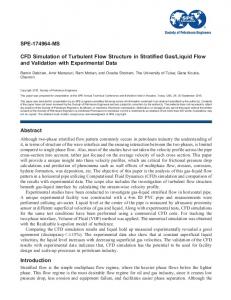
different permeability and thickness (Figure 1 and Table 2). Both injection and production wells are completed over the entire thickness of the model. Depending on which of the boundaries between layers to be preserved or removed, several coarse grid models can be constructed. These models are summarized is Table 3. It is well known that the best way to upscale layered models for two-phase flow is to preserve the layering and minimize the number of grid blocks within each layer. Therefore the best coarse grid model is the one which preserves all layers. This corresponds to non-uniform coarse grid model, case [2]. However a uniform coarse grid model, i.e. case [1], can only preserve the boundary between layers 1 & 2 that is the worst upscaling model based on permeability analysis. In addition the permeability variation and contrast, shown in Table 2, is not equal between different layers. The two top boundaries between layers 2&3 and 3&4, which have the highest permeability change, are more crucial to preserve. Therefore case [3], which preserves these two boundaries, is a better upscaling model than cases [4] and [5] with the same dimension (i.e. 4×3). Vorticity analysis gives similar results about the coarse grid models. In Figure 1 we have mapped vorticity on fourlayer model. As expected, vorticity exists only at the boundary of layers and is zero elsewhere. Nevertheless the intensity of vorticity is different between layers. Two high vorticity zones on top of the model indicate the most important regions to be preserved on coarse grid model in order to achieve better upscaling. From this point of view, cases [2] and [3] which retain these lines can be considered as good upscaled models. This confirms our previous conclusion about the best coarse grid based on analysis of permeability variation. For further evaluation of the coarse grid models, we generated coarse grid vorticity maps. Figures 2a-e represent the refined-based vorticity map for all cases. While case [2] in Figure 2, the non-uniform model which has the same layering as the original fine grid, has preserved fine grid vorticity (both location and intensity), the uniform case [1] has failed to preserve fine grid vorticity, in terms of location of high vorticity and its intensity. This is due to not aligning the coarse grid lines with layering. In cases [3] to [5] although the coarse grid boundaries are aligned with some of the layer boundaries, there is not enough grid lines to preserve all layering.

SPE 110306


Therefore the vorticity zones that appear are correctly positioned, but their intensity is not representative. Hence the result of merging some layers, in these cases, causes that a high vorticity zone vanishes. This effect is more significant for cases [4] and [5], Figures 2d and 2e, which are, as stated earlier, bad cases for upscaling. For more quantitative representation of the above conclusion, we look at the Evmp. Figure 3 compares Evmp of the coarse grid models generated for four-layer model. Evmp inspection suggests that case [1], [4] and [5] should be bad coarse grid models because they have the highest vorticity map preservation error, but cases [2] and [3] could make good models i.e. OCGD because they have small Evmp. The validity of Evmp predictions is confirmed by looking at the two-phase flow simulations results on refined coarse grid models in Figure 3. Both Evmp and two-phase flow error indicators (i.e. Eopr and Ebth ) has the same trend, because homogenization is the main controlling factor on quality of results while numerical dispersion is removed by using refinements. Therefore Evmp is a good mean to evaluate the homogenization error which impacts the accuracy of coarse grid models. As our aim is to use DMM, we now check the prediction made by Evmp for DMM. In Figure 4 the DMM simulation results is presented and compared with those of refined coarse grids. We clearly see that the performance of DMM is very much influenced by structure of coarse grid blocks. According to these results the best coarse grid models suggested by Evmp (cases [2] and [3]) have the best performance on DMM and cases [1] and [5] have the poorest performance. Nevertheless, we observe that case [4], although has very high error regarding preservation of vorticity, could perform very well on DMM. This is an unexpected result that can be verified by looking at the vorticity maps generated from DMM in Figure 5. The vorticity maps using DMM are more detailed than those of refined-coarse grids and are different. Inherent in its procedure, DMM can adapt vorticity map of a coarse grid model in order to represent better the corresponding vorticity field of the fine grid model. This difference between DMMbased vorticity and refined-based vorticity maps, is due to the reconstruction step following application of TW assumption. This reconstruction step creates the vorticity zones that had already been removed due to homogenization and restore them – compare Figures 2a-e and Figures 5a-e. Although the extent of reconstruction depends on the validity of TW assumption and is not the same for all models; the ∆ω is typically smaller than Evmp for all cases. For case [4] DMM has reconstructed fine grid vorticity and that is why the two-phase results of DMM agree very well with fine grid. Figure 6 demonstrates the effect of reconstruction and TW assumption. DMM and refined-coarse grid water cut (fraction of water in the produced fluid) vs. pore volume injected (PVI) for cases [4] and [5] are compared with the fine grid simulation. Refined simulation of the cases shows the significance of homogenization error for both coarse grid models. But better accuracy obtained through incorporating

7

DMM indicates that TW affects the homogenization error implicitly in order to reduce it. However the effectiveness of TW depends on the coarse grid model and is only predictable by ∆ω. But there is a question: can case [4] be an OCGD? The answer depends on the objective of simulation. If we are only interested in the overall and field performance prediction not the detail of model and flow, case [4] can be an OCDG because it has small Eopr and Ebth . But from point of view of geologists and engineers, the best coarse grid model is the one, which best preserves static and dynamic behavior of the fine grid in terms of flow result, and geologic information. This model fails to respect this rule and suffer from high homogenization error due to improper choice of coarse grid blocks. Furthermore, if one decides not to use DMM for flow simulation, therefore the model suggested by DMM-based vorticity may not optimum. Therefore Evmp prediction is more reliable in this case since it chooses the best coarse grid model with least homogenization error which has also minimum error for DMM simulation. It is noteworthy that by using case [2] or [3] in DMM we can save about 30% of the computational time required for the fine grid simulation of four-layer model without any considerable loss of accuracy. Lens Model. The next example considered is a lens

heterogeneity in which a very low permeability ( k = 0.1 mD ), rectangular region is embedded in a high permeability ( k = 100 mD ) background. The fluids in this model tend to move through the high permeability sand and around lens, leaving dead oil within the lens. The location and geometry of this lens has a significant impact on flow and make it difficult to upscale. The location of lens boundaries relative to a uniform 10 by 4 coarse grid is shown in Figure 7. In addition, to make the flow more complicated the displacing fluid (water) is injected to the lower left half thickness and the displaced fluid (oil) is produced from upper right half thickness of the model. In this test case the accuracy of DMM simulation is mainly controlled by homogenization error and the contribution of other sources of error is minor. Therefore the OGCD proposed by vorticity mapping (i.e. Evmp ) is the optimum coarse grid model for DMM too. As shown in Figure 7, none of the coarse grid lines of the uniform 10×4 model (case [1]) coincide with the lens boundaries, which makes it a bad model for upscaling. However it is possible to reduce homogenization error by adjusting grid lines of case [1] (without changing its dimension) in order to align (all or some of) them with lens boundaries. Definitely case [2] which covers all permeability variation boundaries is a perfect model with no homogenization error. Nevertheless we limit ourselves to adjust only two grid lines of case [1] relative to impermeable lens. This creates cases [3] to [6] shown in Figure 9c-f. Based on permeability analysis it is difficult to choose OCGD. For example, case [3] which preserves only the upper and lower boundaries is not preferable to case [4] which preserves only the left and right boundaries. Equally the same situation is held for cases [5] and [6] which preserve the lower-left and

8


upper-right corner boundaries respectively. However we can obtain useful information about the cases by considering vorticity map of the models. Figure 8 displays the vorticity distribution of the fine grid model. No vorticity is created along the vertical lens boundaries, while it is a maximum on the upper and lower boundaries of the lens, although with different signs. The reason for negligible vorticity on vertical boundaries, in spite of large permeability gradient over those boundaries, is that flow is parallel, though very small, to permeability gradient vector. Because fluid prefers to flow in high permeability region, not though the impermeable lens layer. Conversely high flow around the upper and lower boundaries of lens creates a high vorticity zone around those boundaries. In addition, as the flow area is narrower below the lower boundary, the velocity is larger and consequently the vorticity is about 10% higher than the average vorticity observed in the upper part of the lens. Vorticity mapping indicates that the horizontal boundaries of the lens, corresponding to cases [2] and [3], are more important to preserve than the other boundaries; especially the lower boundary of lens which has higher vorticity. This helps to reduce (remove) homogenization error. Therefore case [5] which preserves lower boundary is preferable to case [6]. The argument above is confirmed by looking at vorticity maps of different models in Figure 9. For this model the vorticity generated using the refined coarse grid model and DMM are nearly the same, because homogenization is the most influential factor and the reconstruction step in DMM does not improve the solution. Therefore only DMM vorticity distributions are compared in Figure 9. For further examination we focus on case [4] (Figure 9d) where none of the horizontal lens boundaries are preserved. As seen, there is no vorticity around the lower boundary, while the negative vorticity around the upper boundary has been created above the lens boundary, where there is the coarse grid boundary. It is worth mentioning that DMM cannot reconstruct fine grid vorticity in their actual location. This can be explained by considering the effect of homogenization on fluid flow. As we mentioned earlier there are two high flow regions below and above the lens. The below region is almost blocked to flow, for case [4] and similar cases [1] and [6], due to its very small upscled permeability resulting from merging high permeability (below lens) and low permeability (lens) grid blocks. Hence the fluid fluxes passing through these coarse grid block faces are so small that cannot recreate high flow and consequently high vorticity region beneath the lens. As a result coarse grids corresponding to cases [1], [4], and [6], Figures 9a,d,f are not suitable models with respect to vorticity preservation. In contrast, the models which preserve the lower boundary of lens, consequently the high flow region underneath, are expected to be good models - cases [2], [3], and [5] in Figures 9b,c,e. Focusing again on case [4], we observe a similar effect for the upper high flow region above the lens. In this case, the upper high permeability region remains, but becomes thin. Therefore, most fluid flows through this area that result in an earlier breakthrough time compared with the fine grid model. Again the reconstruction step fails to create the high vorticity region around the upper boundary of lens.

SPE 110306

However, miss aligning of the vertical grid lines relative to the left and right boundaries of the lens has negligible impact on the vorticity map e.g. case [3], Figure 9c. Therefore case [3], as stated earlier, is a good model for upscaling. We now present the actual performance of the coarse grid models in Figure 10. Both Evmp and ∆ω are plotted against oil production and breakthrough errors using DMM. The quantitative results are consistent with the previous qualitative analysis based on vorticity. All those cases preserving the lower lens boundary (i.e. cases [2], [3], and [5]) have low Evmp and are OCGDs. In contrast cases [1], [4], and [6] which have the highest Evmp, demonstrate poor DMM performance. This indicates the dominance of homogenization error on DMM performance predicted successfully by Evmp and the advantages of incorporating vorticity. Computational saving due to employing DMM on the optimum model suggested by vorticity mapping is around 45% compared to the fine grid simulation. Application of the Combined Method to a Real Complex Model (SPE 10, Model 2). The next model considered is a

realistic heterogeneity model taken from the Tenth SPE Comparative Solution Project14, model 2. The original model is 3D comprised of two different portions. The upper portion (layers 1 to 35) is more continues while the lower portion (layers 36 to 85) is highly heterogeneous and channelized. To show the applicability of the combined method (vorticitybased grid generation and DMM), one of the more channelized layers in the lower portion (i.e. layer 59) is considered here. The permeability distribution of the layer as well as the well arrangement and completion are shown in Figure 11. Corey’s type rock relative permeabilities are also used, i.e. ns

ns

 1 − S w − Sr   S w − Sr  kro =   and krw =   where ns = 1 for S − S r   max  Smax − S r  unit mobility ratio displacement and ns = 2 elsewhere, S r = 0.2, and S max = 0.8. Here S w is water saturation. Furthermore the capillary and gravity effects are neglected. We did not use the original fine gird model in our DMM evaluation; instead we upscaled the fine grid (220×60) to a uniform intermediate coarse grid (110×20) to create a computationally less intensive model while the model has almost the same dynamic behavior as the fine gird. This intermediate model was then coarsened to the final upscaling level of 25. Hereafter, this intermediate model is referred to as reference model. Figure 12 shows vorticity distribution for the reference model. Comparing permeability (Figure 11) and vorticity distributions for this model reveals that the vorticity mapping has worked well. Although there are two main high permeability channels, only one branch in the lower part of the model is active (participating to flow), for the well completions used in this model. Therefore, the inactive areas do not appear in the vorticity map, because the velocity component of the vorticity is very small although high permeability gradient exists around the boundaries of high permeability regions. Therefore only this area requires special gridding/refinements and the rest of model can be coarsened.

SPE 110306


For the ultimate upscaling level of 25, several coarse grid models can be generated using the vorticity-based gridding algorithm proposed by Mahani and Muggeridge22 and Ashjari et al.23. Some possible models are listed in Table 4. The dimensions of uniform case [1] (22×4) is selected in order to snap to the gridlines of the reference model (110×20). Dimensions of the other coarse grid models are determined by setting appropriate values for vorticity cut-offs in the horizontal and vertical directions21-23. The constructed coarse grid models are compared in Figure 13 based on Evmp and ∆ω criterions. There is close agreement between the performance predictions by Evmp and ∆ω indicating the dominance of homogenization error. This is plausible since the fine grid model is highly heterogeneous and channelized. The results suggest that significant improvement is achieved by switching from uniform to nonuniform coarsening (compare Evmp for case [1] and e.g. case [5]). This is validated in Figure 13 by including DMM simulation results for unit mobility displacement. The improvement achieved in the accuracy is considerable compared to uniform grid. This improvement is attributed to the selection of proper coarse grid lines which results in better preservation of high permeability channel and reduction of the homogenization error. It can be deduced from Evmps and DMM results that gridding is more favorable and important in the vertical direction (in lower part of the model) than horizontal. This is, in fact, due to the presence of high permeability channel along the model where the high vorticity areas are located. From the DMM results it is observed that the performance of all non-uniform coarse grid models (except case [2]) are quite satisfactory and Eopr and Ebth are less than 3 to 6% respectively. Therefore all of them can be considered as OCGD for the reference model, although case [4] or [5] are the best models (even when mobility ratio changes), both from geological ( Evmp ) and from simulation procedure performance points of view ( ∆ω ). Figure 14 demonstrates how inputting a proper coarse grid model, helps DMM reconstruct reference vorticity on the coarse grid. This is shown for case [5] and case [1] as an example. By incorporating appropriate gridding, the DMM procedure is able to retain the lower high vorticity channel for case [5] while it fails to do so for case [1]. In Figure 15 the sensitivity of DMM results to changing mobility ratio are compared. As seen, case [4] and [5] have almost the highest performances amongst the other coarse grid models and they remain OCGD for different mobility ratios. Finally, the performance of case [5] is examined in Figure 16 against the original fine grid model (220×60). Although the fine grid model is not so large, the speed-up achieved using DMM is magnificent for both uniform case [1] and [5]. In particular, the DMM is four times faster than the fine grid simulation. Staircase Model. This specific model is used to demonstrate

that a combination of homogenization and TW assumption error may control the accuracy of DMM. In the previous models the TW assumption could enhance considerably the

9

performance of DMM where the homogenization error was dominant. However, in this model, the TW assumption causes significant error in simulation, and inputting a model with minimum homogenization error would not be advantageous. The permeability map and the well arrangement used in simulations are shown in Figure 17. The model consists of five stairs with high permeability imbedded in a low permeable background. The injected fluid into the model tends to flow through these high permeable steps. However each step is not extended through the entire length of the model and the fluid has to move from one step to the other in the middle of its trajectory. This causes difficulties in upscaling especially when DMM is incorporated for simulation. The model is designed such that all permeability variation boundaries are aligned with the grid lines of a uniform 10×5 coarse grid model (case [1]). Indeed case [1] is the best coarse grid model with no homogenization error. However we focus on the coarse grid models that could be generated by removing a coarse grid line from uniform case [1]. All possible models (cases [1] to [8]) are shown in Figure 17. The permeability contrast around each boundary is different, with a minimum of 1mD/10mD, maximum of 1mD/1000mD and some values in between. Therefore removing each vertical or horizontal grid line would result in different homogenization errors. From this analysis, case [8] would make a model with minimum homogenization error. Additional information is obtained if we map vorticity on the fine grid model. Each horizontal boundary between steps represents a location of high permeability variation normal to the principal flow direction, which is horizontal in average. Therefore the horizontal step boundaries are potentially locations of vorticity creation. However the calculated vorticity is almost zero around the left and right boundaries of steps although high (horizontal) permeability variation exists Figure 18. This is reasonable because the fluid flux through those boundaries is very small and fluid prefers to flow though high permeability steps not the low permeability background. Due to this fact, the flow direction changes to vertical around these boundaries. Hence, the flow direction becomes parallel with permeability variation and vorticity is not generated. Figure 19 illustrates velocity and vorticity profiles along the boundary between grid block (7,1) and (7,2). As seen the normal component of velocity increases toward the end of boundary and creates a non-uniform velocity and consequently non-uniform vorticity. Figure 20 shows the refined-based vorticity map for all cases. As we have expected the fine grid vorticity is completely preserved by case [1], which preserves all permeability variation boundaries. The effect of eliminating one grid line from case [1] can be observed in the corresponding coarse grid vorticity map. However the effect is not similar for all cases. For instance the vorticity is better preserved for cases which are constructed by removing a vertical grid line (cases [6] to [9]). As shown in Figures 20f to 20i, only length of high vorticity zones has changed compared to the fine grid vorticity, due to the merger of grid blocks around the vertical coarse grid line. The maximum change observed in the length of high vorticity zones is equal to the size of one coarse block of case [1]. However the vorticity length for case [8] is almost unchanged which suggests the

10


case as an OCGD for the staircase model. In contrast the reference fine grid vorticity is not preserved by cases [2] to [5]. These models are less likely to be good coarse grid. The reason is that removing each horizontal grid line from model corresponds to removing a high potential location of forming vorticity. As a result, high vorticity zones in Figures 20b to 20e are formed in the locations different from the corresponding fine grid vorticity. This introduces significant error in vorticity preservation especially for case [4]. In case [5], in addition to vorticity at the horizontal boundaries, a thin high vorticity zone has been created inside the coarse grid block, although the permeability gradient is zero. This can be justified by Equation (3), noting that although fine grid permeability is isotropic, the upscaled permeability is highly anisotropic. Permeability upscaling using PSM, shows a permeability anisotropy of ( k11 ≈ 250k22 ) inside the coarse grid block. Therefore, although the first and second terms in Equation (3) are zero, the last term (anisotropy term) could be considerable depending on the pressure profile and curvature in the block. The above qualitative analysis based on the refined vorticity maps is shown quantitatively in Figure 21. As expected, Evmp is highest for cases [2] to [5] and is lowest for the remaining cases (especially cases [1] and [8]). Twophase flow simulation on the refined coarse grid models confirms Evmp predictions. Both two-phase flow error indicators and Evmp follow almost the same trend. The only exception is case [3] where the model shows a better twophase performance than predicted by Evmp. The reason is in the difference between definitions used for two-phase flow and vorticity preservation errors. In fact, two-phase flow error indicators consider only the errors observed in the production well without taking into account the effect of local errors. In contrast, Evmp gives an average of the errors throughout the model. Although the same overall vorticity preservation error has been calculated for cases [3] and [4], the high Evmp for case [3] is only related to region 1, in Figure 20c, which comprises 20% of the model volume. While in case [4] Evmp is related to region 2, in Figure 20d, which comprises 80% of total volume. Definitely region 2 has a larger impact on fluid flow than region 1, because fluid remains longer in region 2 with wrong vorticity characteristics. However, our main objective is to evaluate DMM performance. Figure 22 presents DMM-based vorticity map for the cases. Interestingly, for case [1] with no homogenization error, DMM has not correctly reconstructed the fine grid vorticity at all points. High vorticity zones are smaller in length; e.g. on the boundary between blocks (7,1) and (7,2) (Figure 22a) there is no vorticity. The reasons are: (1) the main flow direction is vertical, (2) DMM assumes uniform vertical velocity on this boundary (Figure 19). This stems from the TW assumption that distributes fluid flux according to transmissibility. Since vertical transmissibility is uniform, therefore flow is distributed uniformly along the boundary and no vorticity is generated. This is the case in other models too. From the results, we can deduce that (1) the reconstruction step in DMM recreates the missing zones of high vorticity due

SPE 110306

to homogenization, and compensates for homogenization error and even for improper coarse grid structure and (2) the TW assumption does not work in most of the cases and deteriorates the improvement achieved in (1). Therefore the controlling factor on DMM vorticity are both TW and homogenization in these cases, although in some cases TW dominates. For cases [2] to [5] which are bad homogenization models DMM enhances the performance (Figures 22b to 22e) while for cases [6] to [9] which are good homogenized models, no improvement is obtained. This is because the coarsening in these cases is in the x1 direction. TW portioning, although, is applied on both vertical and horizontal faces, its chief negative effect will be on horizontal face, which is longer. Thus TW assumption shortens the high vorticity zones (Figures 22f to 22i) resulting in poor recreation of the fine vorticity in the relevant areas. Similar but more comprehensive comparison of the coarse grid models is given in Figure 23 where ∆ω confirms the previous qualitative vorticity analysis. Recreation of high vorticity zones in cases [2] to [5] results in ∆ω as low as Evmp for case [1]. Furthermore the high ∆ω for good homogenized models (i.e. cases [6] to [9]) demonstrates the dominance of transmissibility weighting assumption. Moreover, Figure 23 shows that two-phase DMM simulation errors follow ∆ω trend not Evmp trend. For instance, case [7] with low homogenization error exhibits poor two-phase DMM performance (Figure 24). This is also not associated with the effect of grid size, but a combination of two abovementioned errors in DMM as shown in Figure 25. Therefore in order to choose the OCGD for the staircase model, we get different answers based on Evmp and ∆ω inspection. Based on ∆ω , case [3] or [4] which have the highest homogenization errors should be selected as OCGD. While based on Evmp , case [7] or [8] should be selected. The final selection depends on the objective of simulation, however a practical solution may be a compromise between solution accuracy and homogenization accuracy; i.e. choosing a model which has the lowest average of ∆ω and Evmp. Alternatively we can use uniform coarse grid, because it is easier to build and may be as accurate enough. Conclusions We presented a novel upscaling technique by combining dual mesh method with vorticity-based gridding. DMM compensates for numerical dispersion by incorporating coarse grid for pressure solution and fine grid for saturation update. But its accuracy is very much dependent on the coarse grid distribution and can be dominated by homogenization error. When homogenization error is dominant, we can remove (reduce) this type of error by inputting proper coarse grid into DMM. The suitability of a coarse grid is confidently predictable by computing Evmp from single-phase flow information (without the need for two-phase flow simulation) for each coarse grid model. We showed that the models, which better preserve the fine grid vorticity, exhibit better performance i.e. lower Eopr & Ebth . This was confirmed by

SPE 110306


two-phase simulation results on Four-layer, Lens models as well as one realistic heterogeneity model. However, in the cases that homogenization error is not dominant, e.g. the error due to TW assumptions is important, the performance of DMM still depends on the structure of coarse grid. But for these cases the optimum coarse grid model cannot be determined only by Evmp inspection. The DMMbased vorticity error ( ∆ω ) is a good predictive tool in these cases. Nevertheless, the optimum coarse grid model suggested by ∆ω is not always a good representative of fine grid model in terms of static and dynamic flow features. In practice, therefore, we may either choose the model with minimum average ∆ω and Evmp or simply a uniform coarse grid. Furthermore, for all cases considered here, the combination of vorticity and DMM (i.e. non-uniform DMM) resulted in a less computationally demanding and more accurate upscaling technique. Acknowledgments The authors gratefully acknowledge Dr. Pascal Audigane for providing us invaluable help regarding dual mesh method code and Prof. Martin Blunt for his useful comments. Nomenclature Ebth = breakthrough time error Eopr = root mean squares of oil production error = refined-based vorticity map preservation Evmp error = IMplicit Pressure Explicit Saturation IMPES scheme r r r = unit vectors i , j, k k k =  11  k21

k12  k22 

= permeability tensor

k*

= effective block permeability tensor

kr

M m N

= phase relative permeability = maximum grid size in the computational domain = mobility ratio = number of grid lines in x1 direction = total number of coarse grid blocks

n

= number of grid lines in x2 direction

n2

= number of fine grid cells at coarse grid block face = exponent for the Corey’s type relative permeability model = optimal coarse grid distribution

l

ns

OCGD P PSM PVI q

= fluid pressure = Pressure Solver Method = Pore Volume Injected = fluid flux at the boundary between two grid blocks

qo S S max Sr

11

t tbth

= oil production rate = phase saturation = maximum saturation = residual saturation = transmissibility weighting = transmissibility in the x1 direction between grid blocks i and i + 1 = time = breakthrough time

tsf

= final simulation time, tsf =

TW T1,i+1 2

∑ n

l

∆ti

1

r V

= single-phase velocity vector r r r r ( V = v1i + v2 j + v3 k )

xi

= Cartesian coordinates ( i = 1, 2,3 )

Greek Symbols ∆t = sampling time step (controlled by simulator) = fine grid cell size in the xi direction ∆xi ( i = 1, 2,3 ) =overall difference between fine grid and ∆ω DMM-based vorticity φ = porosity

λt r

ω ∇ ∇.

= total mobility = single-phase vorticity vector r r r r ( ω = ω1i + ω2 j + ω3 k ) = gradient operator = divergence operator

Superscripts c = coarse grid model f = fine grid model DMM = dual mesh method Subscripts o = oil w = water References 1. Jones, A.D.W., Verly, G.W. and Williams, J.K., “What Reservoir Characterization is Required for Predicting Waterflood Performance in a High Net-to-Gross Fluvial Environment?”, North Sea Oil and Gas Reservoirs-III (1994) 223-232. 2. Durlofsky, L.J. et al., “Scale-up of Heterogeneous Three Dimensional Reservoir Descriptions”, paper SPE 30709 presented at the 1995 SPE Annual Technical Conference and Exhibition, Dallas, October 22-25. 3. Jones, A.D.W., “Which Subsurface Heterogeneities Influence Waterflood Performance? A Case Study of a Low Net to Gross Fluvial Reservoir”, New Developments in Improved Oil Recovery (edited by De Haan H.J.), Geological Society Special Publication (1995) 84: 5-18. 4. Durlofsky, L.J., “Upscaling of Geocellular Models for Reservoir Flow Simulation: A Review of Recent Progress”, 7th International Forum on Reservoir Simulation Bühl/Baden-Baden, Germany, June 23-27 (2003).

12


5. Christie, M.A., “Upscaling for Reservoir Simulation”, Journal of Petroleum Technology (1996) 1004-1010. 6. Barker, J.W. and Thibeau, S., “A Critical Review of the Use of Pseudo Relative Permeabilities for Upscaling”, SPE Reservoir Engineering (1997) 12: 138-143. 7. Renard, P. and de Marsily, G., “Calculating Equivalent Permeability: A Review”, Advances in Water Resources (1997) 20: 253-278. 8. Durlofsky, L.J., Jones, R.C. and Milliken, W.J., “A Nonuniform Coarsening Approach for the Scale-up of Displacement Process in Heterogeneous Porous Media”, Advances in Water Resources (1997) 20 (5-6): 335-347. 9. Wen, X.H., Durlofsky, L.J. and Edwards, M.G., “Upscaling of Channel Systems in Two Dimensions Using Flow-Based Grids”, Transport in Porous Media (2003) 51: 343–366. 10. Garcia, M.H., Journel, A.G. and Aziz, K., “Automatic Grid Generation for Modeling Reservoir Heterogeneities”, SPERE (1992) 7: 278-284. 11. Durlofsky, L.J., Jones, R.C. and Milliken, W.J., “A New Method for the Scale up of Displacement Processes in Heterogeneous Reservoir”, Proceeding of the 4th European Conference on the Mathematics of Oil Recovery, Roros, Norway (1994). 12. Li, D., Cullick, A.S. and Lake, L.W., “Global scale-up of reservoir model permeability with local grid refinement”, Journal of Petroleum Science and Engineering (1995) 14: 1-13. 13. Durlofsky, L.J., Behren, R.A. and Jones, R.C., “Scale Up of Heterogeneous Three Dimensional Reservoir Description”, SPE Journal (1996) 1: 313-326. 14. Christie, M.A. and Blunt, M.J., “Tenth SPE comparative solution project: A comparison of upscaling techniques”, SPE Reservoir Evaluation and Engineering (2001) 4: 308-317. 15. Qi, D.S., Wong, P.M. and Liu, K. Y., “An improved global upscaling approach for reservoir simulation”, Petrol. Sci. Technol. (2001) 19: 779-795. 16. Qi, D.S., and Hesketh, T., “REV grid technique for reservoir upscaling”, Petroleum Science and Technology (2004) 22: 15951624. 17. Soleng, H.H. and Holden, L., “Gridding for Petroleum Reservoir Simulation”, In: Numerical Grid Generation in Computational Field Simulations, edited by Cross, M., Soni, B.K., Thompson, J.F., Hauser, J. and Eiseman, P.R., Missisipi State University (1998). 18. He, C., “Structured Flow-based Gridding and Upscaling for Reservoir Simulation”, PhD thesis, Petroleum Engineering Department, Stanford, Stanford University (2004). 19. Wen, X.H., Gómez-Hernández, J.J., “Selective Upscaling of Hydraulic Conductivities”, Geostatistics Wollongong, vol. 2, 1112-1123, edited by E. Y. Baafi and N. A. Schofield, Proceedings of the Fifth International Geostatistics Congress, Wollongong, Australia, 22-27 September (1996). 20. Wen, X.H., Gómez-Hernández, J.J., “Upscaling Hydraulic Conductivities in Crossbedded Formations”, Mathematical Geology (1998) 30(2): 181-212. 21. Mahani, H., “Upscaling and Optimal Coarse Grid Generation for the Numerical Simulation of Two-Phase Flow in Porous Media”, PhD thesis, Department of Earth Science and Engineering. London, Imperial College London (2005). 22. Mahani, H., Muggeridge, A.H., “Improved Coarse Grid Generation Using Vorticity”, SPE paper 94319 presented at the 14th annual SPE/EAGE conference, Madrid, Spain, June 13-16 (2005). 23. Ashjari, M.A., Firoozabadi, B., Mahani, H. and Khoozan, D., “Vorticity-based Coarse Grid Generation for Upscaling TwoPhase Displacements in Porous Media”, Journal of Petroleum Science and Engineering (2007)doi:10.1016/j.petrol.2007.04.006.

SPE 110306

24. Artus, V., Noetinger, B., “Up-scaling Two-Phase Flow in Heterogeneous Reservoirs: Current Trends”, Oil & Gas Science and Technology - Rev. (2004) 59 (2): 185-195. 25. Audigane, P., Blunt, M.J., “Dual Mesh Method for Upscaling in Waterflood Simulation”, Transport in Porous Media (2004) 55: 71-89. 26. Gautier, Y., Blunt, M.J., Christie, M.A., “Nested Gridding and Streamline-Based Simulation for Fast Reservoir Performance Prediction”, Computational Geosciences (1999) 3:295-320. 27. Begg, S. H., Carter, R.R. and Dranfield, P., “Assigning Effective Values to Simulator Grid block Parameters for Heterogeneous Reservoirs”, SPE Reservoir Engineering (1989) 4: 455-463. 28. Aziz, K. and Settari, A., “Petroleum Reservoir Simulation”, Applied Science Publishers, London, (1979). 29. Rame, M., Killough, J.E., “A New Approach to the Simulation of Flows in Highly Heterogeneous Porous Media”, paper SPE 21247 presented at the SPE symposium on Reservoir Simulation, Anaheim (1991). 30. Guérillot, D.R., Verdière, S., “Different Pressure Grids for Reservoir Simulation in Heterogeneous Reservoirs”, paper SPE 29148 presented at the SPE Symposium on Reservoir Simulation, San Antonio, Texas, 12-15 February (1995). 31. Guedes, S.S., Schiozer, D.J., “An Implicit Treatment of Upscaling in Numerical Simulation”, paper SPE 51937 presented at the SPE Symposium on Reservoir Simulation, Houston, 14-17 February (1999). 32. Hermitte, T., Guérillot, D., “A More Accurate Numerical Scheme for Locally Refined Meshes in Heterogeneous Reservoirs”, paper SPE 25261 presented at the SPE Symposium on Reservoir Simulation, New Orleans, 28 February–3 March (1995). 33. Chen, Y., “Upscaling and Subgrid Modeling of Flow and Transport in Heterogeneous Reservoirs”, PhD thesis, Petroleum Engineering Department, Stanford University, Stanford (2005). 34. Chen, Y. and Durlofsky, L.J., “Adaptive Local-Global Upscaling for General Flow Scenarios in Heterogeneous Formations”, Transport in Porous Media (2006) 62: 157-185. 35. Efendiev, Y.R. and Hou, T.Y., “Multiscale Finite Element Methods for Porous Media Flows and their Applications”, Applied Numerical Mathematics (2007) 57(5-7): 577-596. 36. Efendiev, Y.R., Hou, T.Y., and Wu, X.H., “Convergence of a nonconforming multiscale finite element method”, SIAM J. Numer. Anal. (2000) 37: 888-910. 37. E, W. and Engquist, B., “The Heterogeneous Multiscale Methods”, Comm. Math. Sci. (2003) 1: 87-132. 38. Efendiev, Y.R., and Durlofsky, L.J., “A Generalized ConvectionDiffusion Model for Subgrid Transport in Porous Media”, Multiscale Model. Simul. (2003) 1(3): 504-526. 39. Wen, X.H. and Gomez-Hernandez, J.J., “Upscaling Hydraulic Conductiveties in Heterogeneous Media: An Overview”, J. Hydrology (1996) 183: ix-xxxii. 40. Wen, X.H., Durlofsky, L.J. and Edwards, M.G., “Use of Border Regions for Improved Permeability Upscaling”, Mathematical Geology (2003) 35(5): 531-547. 41. Chen, Y., Durlofsky, L.J., Gerritsen, M., and Wen, X.H., “A Coupled Local-Global Upscaling Approach for Simulating Flow in Highly Heterogeneous Formations”, Advances in Water Resources (2003) 26: 1041-1060. 42. Efendiev, Y.R., and Durlofsky, L.J., “Accurate subgrid models for two-phase flow in heterogeneous reservoirs”, SPE Journal (2004) 9(2): 219-226.

SPE 110306


Tables and Figures

13

(d)

(e) Figure 1. The finely gridded permeability field and the normalized vorticity map calculated for four-layer system. The highest vorticity is observed at the boundary between the top layer and the layer immediately beneath it where there is the highest velocity and the highest permeability contrast. (a)

Figure 2. Refined-based vorticity map for coarse grid models (listed in Table 3) constructed for four-layer model. Vorticity is only created around the boundaries of permeability variation and inside each layer vorticity is zero.

(b)

(c) Figure 3. Refined-based vorticity map preservation error ) for coarse grid models, shown in Figure 2, is ( 0.5 Evmp compared with 0.7 Eopr ( mobility displacement.

) and 0.25 Ebth (

) for unit

14


SPE 110306

(d)

(e)

Figure 4. 0.5 Evmp (

) and ∆ω (

) are compared with

DMM two-phase simulation error indicators 0.5 Eopr (

) and

). Both Evmp and ∆ω have the same predictions except for case [4]. The high homogenization error observed in case [4] is eliminated during reconstruction step in DMM.

0.3Ebth (

(a) Figure 5. DMM-based vorticity maps of the coarse grid models for cases shown in Figure 2. DMM has reconstructed some missing high vorticity zones compared with Figure 2. (a)

(b)

(b)

(c)

Figure 6. Four-layer model. Comparison of water fractional flow vs. PVI between fine grid solution and coarse grid solutions obtained by DMM and Refined-coarse grid models, (a) case [4], (b) case [5].

SPE 110306


15

(c)

Figure 7. Lens permeability map and well arrangement. The boundaries of lens are not aligned with the uniform coarse grid lines (10×4).

(d)

(e) Figure 8. Fine grid vorticity map of lens model. Bold lines represent injection and production wells. High vorticity zones are located on the lens horizontal boundaries. No vorticity is generated around the vertical boundaries of lens. (a)

(f)

(b)

Figure 9. DMM-based vorticity map of the coarse grid models generated for lens model. All high vorticity zones are formed on the boundaries between coarse blocks due to permeability gradient. The reconstruction step in DMM is unable to recreate fine grid vorticity.

16


Figure 10. Comparison of DMM two-phase error indicators ( Eopr , and Ebth ) and Evmp ( ) and ∆ω ( ). Homogenization error is dominant for lens model, hence both Evmp and ∆ω have the same predictions.

SPE 110306

Figure 13. Performance prediction of the coarse grid models ) and 2 × ∆ω ( ). Cases (listed in Table 4) using 2 × Evmp ( [4] and [5] with minimum Evmp are considered as OCGD for layer 59 intermediate model. The predictions are confirmed by two-phase DMM error indicators ( 2 × Eopr , Ebth ) for unit mobility displacement. (a)

Figure 11. Permeability field of layer 59 (220×60) of SPE 10th, Model 214 formed of two high permeability channels. The bold lines on the left and right side of the model are injection and production wells.

Figure 12. Vorticity map of intermediate fine grid model (110×20) which is the upscaled model of the original model of layer 59 with dimension 220×60.

(b)

Figure 14. Comparison of DMM-based vorticity map for (a) case [1] and (b) case [5]. Fine grid vorticity has been reconstructed by DMM for case [5].

SPE 110306


17

Figure 18. Fine grid vorticity map for staircase model. The high vorticity zones are only observed on the boundary between steps. Close to the end of each step flow becomes vertical, so vorticity becomes zero. Figure 15. Effect of mobility ratio (M) on DMM performance for the coarse grid models generated for layer 59 intermediate fine grid model. Mobility change has minor effect on the performance of cases [4] and [5].

Figure 16. Water fractional flow for the original fine grid, layer 59 (220×60) for unit mobility displacement. The combined vorticity-based gridding and DMM (case [5]) shows significant accuracy and computational saving compared with uniform case [1].

Figure 19. Comparison of the normal velocity and vorticity distribution along the boundary between blocks (7,1) and (7,2). DMM assumes uniform velocity and vorticity profiles, while in the fine grid they are non-uniform. (a)

(b)

Figure 17. Permeability distribution for staircase model. There is no homogenization error for uniform 10×5 case [1]. The number in front of each coarse grid line represents the corresponding coarse grid model that is constructed by removing that grid line from case [1]. Cases [2] to [5] have slightly more upscaling level than cases [6] to [9].

18


SPE 110306

(c)

(d)

(e)

(i)

Figure 20. Refined-based vorticity map of coarse grid models constructed for staircase model. Only uniform case [1] is able to fully preserve the vorticity of finely gridded model. Cases constructed by removing a vertical grid line (cases [6] to [9]) preserve better the fine grid vorticity.

(f)

(g)

Figure 21. The homogenization error for different coarse grid models constructed for staircase model is estimated using 2 × Evmp ( ). Cases [1] and [8] with minimum Evmp are considered as OCGDs for the model. Two-phase simulation 2 × Eopr , Ebth ) on the refined system confirm the results ( predictions by Evmp.

SPE 110306


(a)

(f)

(b)

(g)

(c)

(h)

(d)

(i)

(e)

19

Figure 22. DMM-based vorticity maps of the coarse grid models constructed for staircase model. The fine grid vorticity is better reconstructed by cases [2] to [5] than cases [6] to [9].

20


SPE 110306

Table 1. Properties of simple synthetic models four-layer, lens, and staircase model for unit mobility displacement. Size Grid block sizes Viscosities Porosity n m ∆x1 ∆x 2 ∆x3 oil water

φ = 0.2

100

20

7.62 m

7.62 m

7.62 m

1 cp

1 cp

Table 2. Properties of each layer of four-layer model. The last two rows show permeability change and ratio between layers. The boundary between layers 3 and 4 experiences the highest permeability variation. Layer Number 1 2 3 4 Thickness ( m) 38.1 60.96 38.1 15.24 Figure 23. Two-phase DMM simulation errors (

2 × Eopr ,

Ebth ) are predicted by 2 × Evmp ( ) and ∆ω ( ). Performance predictions made by Evmp and ∆ω are quite different.

Permeability (mD ) Normal Change of Permeability Permeability contrast (ratio)

1.0

10.0

100.0

0.1

9.0

90.0

99.9

0.1

0.1

1000.0

Table 3. Several coarse grid models constructed for four-layer model (with dimension 100×20). SL and EL corresponds to the number of fine layer where a coarse layer starts and ends. In the horizontal direction (i.e. x1 ) the size of coarse blocks are uniform. Size Case 1 (Uni.) 2 3 4 5

Figure 24. Water fractional flow for staircase model. Simulation result on the refined coarse grid (case [7]) is in good agreement with fine grid, but there is large discrepancy between DMM and fine grid results.

Coarse grid Layer Number 2 3 4 EL SL EL SL EL SL EL

nc

mc

SL

4

4

1

5

6

10

11

15

16

20

4 4 4 4

4 3 3 3

1 1 1 1

5 13 5 5

6 14 6 6

13 18 18 13

14 19 19 14

18 20 20 20

19 -

20 -

Table 4. Several coarse grid models generated for fine grid model of layer 59 (intermediate 110×20 model) using vorticity-based grid generation algorithm21-23. Upscaling Size Level Case Fine (intermediate) 1(uniform) 2 3 4 5 6 7

Figure 25. The effect of grid size on DMM simulation result on case [7]. Case [7] 10×5 has the same grid resolution and structure as the case [1], but its permeability distribution is the same as original Case [7] 9×5.

1

nc

mc

110

20

-

22 22 15 11 9 7 5

4 4 6 8 10 13 17

25.0 25.0 24.4 25.0 24.4 24.1 25.9

SPE 110306 Reservoir Flow Simulation Using

SPE 110306 Reservoir Flow Simulation Using

Suggest Documents

PETROLEUM RESERVOIR SIMULATION USING ...

SPE-171611-MS Integrated Geoscience and Reservoir Simulation ...

SPE 95789 Incorporating 4D Seismic Data in Reservoir Simulation ...

SPE 53671 Reservoir Flow Units: A Comparison ...

SPE 100573 Analysis of Gas Well Reservoir Performance Data Using ...

SPE-173271-MS Fast Multiscale Reservoir Simulations using POD ...

Constructing Reservoir Flow Simulator Proxies Using Genetic ...

upscaling reservoir simulation using multilevel ...

Field Development Planning Optimization Using Reservoir Simulation

reservoir daily inflow simulation using data fusion

SPE-174964-MS CFD Simulation of Turbulent Flow ... - OnePetro

SPE 169564 Estimation of Stimulated Reservoir ...

SPE 106679 Permeability Upscaling Techniques for Reservoir ...

SPE 134934-PP Improved Reservoir Management ...

SPE 173237 Rapid Reservoir Modeling: Prototyping ...

A two-phase flow simulation of a fractured reservoir ...

Hybrid Mesh Generation for Reservoir Flow Simulation in CPG Grids

Staggered In Time Coupling of Reservoir Flow Simulation and ...

Compositional Reservoir-Flow Simulation for Organic-Rich ... - OnePetro

Simulation of Subsurface Two-Phase Flow in an Oil Reservoir

Three-dimensional reservoir characterisation and flow simulation of ...

Enhanced Geothermal Reservoir Simulation

RESERVOIR SIMULATION - eolss

SPE 120668 Well Test Simulation using Orthogonal ...