SPEAR - Longline Environment

Sustainable Options for People, Catchment and Aquatic Resources The SPEAR Project, an International Collaboration on Integrated Coastal Zone Management

J.G. Ferreira, H.C. Andersson, R.A. Corner, X. Desmit, Q. Fang, E.D. de Goede, S.B. Groom, H. Gu, B.G. Gustafsson, A.J.S. Hawkins, R. Hutson, H. Jiao, D. Lan, J. Lencart-Silva, R. Li, X. Liu, Q. Luo, J.K. Musango, A.M. Nobre, J.P. Nunes, P.L. Pascoe, J.G.C. Smits, A. Stigebrandt, T.C. Telfer, M.P. de Wit, X. Yan, X.L. Zhang, Z. Zhang, M.Y. Zhu, C.B. Zhu S.B. Bricker, Y. Xiao, S. Xu, C.E. Nauen, M. Scalet. IMAR – Institute of Marine Research http://www.imar.pt

SPEAR team J.G. Ferreira J. Lencart-Silva A.M. Nobre J.P. Nunes Y. Xiao

IMAR - Institute of Marine Research, Centre for Ocean and Environment, New University of Lisbon, Portugal

A.J.S. Hawkins S.B. Groom R. Hutson P.L. Pascoe

Plymouth Marine Laboratory, United Kingdom

T.C. Telfer R.A. Corner

Institute of Aquaculture, University of Stirling, United Kingdom

A. Stigebrandt H.C. Andersson B.G. Gustafsson

University of Gothenburg, Sweden

J.G.C. Smits X. Desmit E.D. de Goede

Deltares, Netherlands

M.Y.Zhu R. Li X. Liu X.L. Zhang Z. Zhang

First Institute of Oceanography, State Oceanic Administration, China

X. Yan H. Jiao Q. Luo S. Xu

Ningbo University, China

D. Lan Q. Fang H. Gu

Third Institute of Oceanography, State Oceanic Administration, China

J.K. Musango

CSIR, South Africa

M.P. de Wit

De Wit Sustainable Options (Pty) Ltd, South Africa

C.B. Zhu

South China Sea Fisheries Research Institute, CAFS, China

S.B. Bricker

Center for Coastal Monitoring and Assessment, NOAA, USA

C.E. Nauen

European Commission, Brussels, Belgium

M. Scalet

European Commission, Brussels, Belgium

3

Foreword This book describes the approach and main results obtained in the Sustainable options for PEople, catchment and Aquatic Resources (SPEAR) Project, together with complementary case studies focusing on related work in China and in the United States. Each chapter in this book is designed to be readable by itself, and contains enough information for the reader to understand both the methodologies applied and the key outcomes. Wherever possible, those outcomes have been developed into products, with the objective of leveraging their usability as a legacy of SPEAR. From a technical standpoint, these products currently represent the state-of-the-art in coastal management, featuring web-based models, hybrid ecological-economic approaches, and management tools to be used at a variety of scales. Technological developments will mean that the tools themselves will evolve fairly rapidly, but the underlying scientific paradigms are expected to change more slowly. Models do not by themselves lead to robust management, without a complementary investment in appropriate environmental data. Management-oriented work in Integrated Coastal Zone Management (ICZM) often results in multidisciplinary actions, rather than an interdisciplinary approach. As a consequence, there is often a lack of integration which is limiting to coastal management. Three aspects of this merit further analysis: (i)

The lack of effective interaction between natural and social sciences, the acknowledgement of the limitations and errors of each, and the recognition that ICZM can only be appropriately addressed by a well integrated approach;

(ii)

The understanding that environmental baselines are shifting, in some cases rather rapidly, and that the record of that shift is often at best anecdotal;

(iii) The realisation that tools such as those developed in SPEAR are of maximum utility when all social agents, such as environmental and fisheries agencies, farm stakeholders, non-governmental agencies and other parties are actively involved.

This book does not aim to provide an exhaustive account of all the research executed in SPEAR, and the reader is directed to the official project website, available in English at http:// www.biaoqiang.org/ and in Chinese at http://www.spear.cn/ A digital copy of this book is available on the site, together with links to databases, models and all other resources made available by this research.

4

6

7

8

9

10

oyster cage area coastal features coastal pond

11

1600

Modelled mean growth (g)

1400 R2 = 0.9233

1200 1000

R2 = 0.9515

800 600 400 200 0

0

200

400

600

800

1000

Observed mean growth (g)

12

1200

1400

1600

13

Shellfish filtration

EUTROPHICATION CONTROL Phytoplankton removal 2608 Kg C y-1 Detritus removal 972 Kg C y-1 N removal (kg y-1)

Population equivalents 122 PEQ y-1

ASSETS Chl a O2 Score

14

Algae Detritus Excretion Faeces Mass balance

INCOME Shellfish farming: Nutrient treatment: Total income:

-406 -151 24 129 -404

PARAMETERS 77.3 k€ y-1 36.7 k€ y-1 114.0 k€ y-1

Density: 20 oysters m-2 Cultivation period: 365 days 20% mortality 3.3 kg N y-1 PEQ

15

16

Aquaculture zones Fishcages Kelp Bivalves

Scenario 1

Scenario 2 Scenario 3

17

18

Executive Summary In 2004, the European Union financed a research project entitled Sustainable options for PEople, catchment and Aquatic Resources (SPEAR). This project was framed in the INternational COoperation for DEVelopment (INCO-DEV) programme, with its focus on mutually beneficial and equitable partnership in research between the Community and its Member States on the one hand and INCO target countries on the other. The general objective of SPEAR was to develop and test an integrated framework for management of the coastal zone, using two test cases where communities depend primarily upon marine resources. Two contrasting coastal systems in China were used as study areas. Sanggou Bay is in a rural area in the North, and Huangdun Bay is in an industrialized area south of Shanghai, subject to substantial human pressure at both local and regional levels. The common denominator for both is that aquatic resources, i.e. cultivated species of seaweeds, shellfish and finfish, are of paramount importance for community income and livelihood, both locally and regionally. This book describes the approach and main results obtained, together with complementary case studies focusing on related work in China and in the United States. The book is divided into seven chapters, followed by a Conclusions section. Each of the chapters is designed to be readable by itself, allowing different publics to find their sections of interest without needing to refer extensively to other material. A brief description of each chapter is given below.

19

Rationale for the SPEAR Project The motivation and objectives for this work are explained here, together with an overview of the way in which this project fits into the wider context of coastal zone management. The key objectives of SPEAR are outlined below, focusing on integration of disciplines and tools as a primary element, and specifically associating ecology and economics as the two major components of the framework. Later chapters illustrate how the various parts were brought together, and provide specific examples of applicability. Main objectives of SPEAR Develop an integrated framework that simulates the dynamics of the coastal zone accounting for basin effects (exchanges of water, sediment and nutrients), ecological structure and human activities Test this framework using research models, which assimilate dispersed local and regional data, and develop screening models which integrate key processes and interactions Examine ways of internalizing environmental costs and recommend response options such as optimisation of species composition and distributions, thereby restoring ecological sustainability Evaluate the full economic costs and benefits of alternative management strategies, and societal consequences Provide managers with quantitative descriptors of environmental health, including simple screening models, as practical diagnostic tools

There is a chapter dedicated to an overview of the various tools, which will guide a reader who is fundamentally interested in knowing what scientific and technical instruments are available to support coastal management.

20

Tools This chapter provides a description of data, remote sensing and modelling tools, crosscutting the different scientific disciplines.

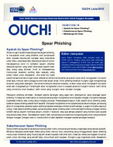
oyster cage area coastal features coastal pond

FIGURE 1. Huangdun Bay: (Left) Landsat band 5, near IR scene showing coastal features and fish cages. (Right) Diagram of main aquaculture provided by Chinese partners.

Figure 1 shows an example of these tools, illustrating how satellite data were combined with ground truthing data and local knowledge to generate final aquaculture maps.

Systems This chapter provides the grounding for the system-scale modelling work. Models can only ever be as good as the data that drive them, so a robust data programme is a key element for success. China

Shandong province

Sanggou Bay

ZheJiang province

Huangdun Bay (Ningbo City)

Population (million)

1 300

≅ 92

≅ 0.15

≅ 47

6

Urban per capita disposable income (USD)

1 290

≅ 860

≅ 2000 (Weihai) ≅ 560 (Jinan) ≅ 460 (Yantai)

1 260

3 300

Primary sector share of economy (%)

15%

11%

n/a

7%

7%

47 061 064

7 062 244

188 227

4 935 288

903 301

Fish production (tons)

21

Total fisheries value (RMB millions)

332 341

37 600

5 897

13 859

n/a

Related industry value (RMB millions)

126 186

40 208

9 212

3 083

n/a

Related services value (RMB millions)

119 357

22 505

500

292

n/a

Marine farming value (RMB millions)

73 375

16 797

1 364

n/a

n/a

Total fisheries jobs

7 007 564

n/a

n/a

n/a

n/a

Fish farming jobs

4 324 174

n/a

n/a

n/a

n/a

n/a

n/a

11 100

n/a

n/a

Marine farming jobs

FIGURE 2. Selected socio-economic indicators for the regions (compiled from FAO 2004, China Data Centre, National Bureau of Statistics of China).

Data collation was a key element of the work, data collection was only carried out as required, with a view to optimising costs and leveraging previous work. A horizontal approach to this part of the work meant that both the catchment and waterbody were considered, and that there was a close integration of the various scientific disciplines involved. Figure 2 shows an example of the data collected for the two bays. Both Shandong and Zhejiang provinces are less dependent on the primary sector than China in general, but Shandong is more dependent on primary production than Zhejiang. The total value of all fisheries production and the value of marine farming is also markedly higher in Shandong where 45% of the total fisheries value is in marine farming. In China as a whole 4.2 million people are employed in the fish farming (inland and marine) business. This means that almost 19 direct fish farming jobs are created per RMB 1 million of value in fish farming. Comparative statistics for the provinces were not available, but for marine farming only in Sanggou Bay this figure is around 9 direct jobs per RMB 1 million in total marine farming value.

22

Aquaculture This chapter provides a full description of aquaculture activity within the two bays, highlighting the areas involved, key features of the culture practice, and socio-economic aspects. In addition, the models used to describe growth and waste production for seaweeds, shellfish (both bivalves and shrimp), and finfish are described here. 1600

Modelled mean growth (g)

1400 R2 = 0.9233

1200 1000

R2 = 0.9515

800 600 400 200 0

0

200

400

600

800

1000

1200

1400

1600

Observed mean growth (g) FIGURE 3. Modelled growth (TGC model) against empirical data for Japanese seabass (black) and yellow croaker (blue) grown in Huangdun Bay.

As an example, Figure 3 shows a comparison of modelled and observed fish growth of species in Huangdun Bay, simulated using a Thermal Growth Coefficient model.

23

Ecosystem models The system-scale data were combined with aquaculture data to provide the information required to run ecosystem-scale models. SPEAR system-scale models Fine-scale models, simulating the three-dimensional water circulation in both bays Broader-scale water quality models, simulating key features of water and sediment properties Coarse-scale ecological models, which represent the systems using a few dozen boxes, but contain all the necessary elements of the ecological and human components, and simulate multi-year periods Economic models, coupled to the ecological models, in order to explicitly account for the interactions between the human system and the ecosystem

The integration of the various models was carried out both online (with models running together and interacting with each other) and using offline coupling, with results from one model being used to drive another model. The essence of this was to capture the scales at which important phenomena occur, since it is clearly impossible to use the same time and space scales to simulate the detailed water circulation over a tidal cycle and the decadal production of oysters. Box 1

Box 2

Box 3

Box 4

Box 5

Box 6

Box 7

Box 10

Total

Oyster (model)

9817

8948

1534

6912

8810

-

-

-

36021

Oyster (data)

9764

8976

1500

6860

7220

-

-

-

34320

Razor (model)

808

568

471

52

115

46

-

-

2058

Razor (data)

812

588

415

57

95

30

-

-

1997

Manila clam (model)

134

102

91

26

26

7

39

6

431

Manila clam (data)

116

84

108

26

27

8

37

5

410

Muddy clam (model)

355

316

174

-

35

23

-

-

903

Muddy clam (data)

394

286

199

-

26

14

-

-

920

Figure 4. EcoWin2000 shellfish harvest results and comparison with data for Xiangshan Gang (ton yr-1).

24

A synthesis illustrating final outputs from these models, which are of clear management interest, is shown in Figure 4 for Xiangshan Gang. The data compare the results from the EcoWin2000 ecological model to reported production for four shellfish species in Xiangshan Gang. In order to produce such results, a diverse set of models needs to be combined, including hydrodynamic models such as Delft3D, shellfish individual growth models such as ShellSIM, models of fish production and waste such as MOM, and economic models such as MARKET.

Screening models SPEAR also focused on the development and implementation of screening models, which have a totally different objective and user-base than the research models referred above. A screening model is a tool that may be useful for a fish farmer, farm manager or coastal manager. Typically these models are easy to use, run in minutes, and support decisions such as the assessment of the impact of a particular planning option or classification of the ecological status of an aquatic system. Two examples of application of this type of model are provided below. Particulate waste models At the local scale, screening models may be used to look at aquaculture yields, local impacts of fish farming, and water quality. A good example is a particulate waste distribution model developed for fish culture in Huangdun Bay (Figure 5) using GIS, which provides a footprint of organic enrichment beneath fish farms.

Figure 5. Screening model for carbon input to sediments from fish culture.

25

FARM The Farm Aquaculture Resource Management (FARM) modelling framework applies a combination of physical and biogeochemical models, bivalve growth models and screening models for determining shellfish production and for eutrophication assessment. Requirements for input data have been reduced to a minimum, since the model is aimed at the shellfish farming community and local managers. Model inputs may be grouped into data on: (i) farm layout, dimensions, species composition and stocking densities; (ii) suspended food entering the farm; and (iii) environmental parameters. The FARM model is publicly available at http://www.farmscale.org/

Shellfish filtration

EUTROPHICATION CONTROL Phytoplankton removal 2608 Kg C y-1 Detritus removal 972 Kg C y-1 N removal (kg y-1)

Population equivalents 122 PEQ y-1

ASSETS Chl a O2 Score

Algae Detritus Excretion Faeces Mass balance

INCOME Shellfish farming: Nutrient treatment: Total income:

-406 -151 24 129 -404

PARAMETERS 77.3 k€ y 36.7 k€ y-1 -1

114.0 k€ y-1

Density: 20 oysters m-2 Cultivation period: 365 days 20% mortality 3.3 kg N y-1 PEQ

Figure 6. Application of FARM to calculate a mass balance for oyster culture in Sanggou Bay

The application of FARM to an oyster farm in Sanggou Bay is shown in Figure 6, and illustrates the substitution value of shellfish with respect to land-based control of nutrient emissions. In a scenario of integrated catchment management of discharges of nitrogen and phosphorus, such as already occurs in parts of the U.S. and in Scandinavia, shellfish farmers in Southeast Asia may in future be able to sell nutrient credits to their land-based counterparts in much the same way as carbon credits are traded today.

26

Management and case studies The tools developed within SPEAR are designed to support decision-makers in successfully implementing integrated castal zone management (ICZM), harmonising various (often competing) uses into a framework for sustainable development. The project team worked closely with stakeholders to develop a set of example scenarios (Figure 7) which could be examined using the SPEAR models. System

Scenario description

Tools

Huangdun Bay

Assess impact of change to fish cage numbers and sizes

GIS, EcoWin2000

Assess impact of nutrient discharge reduction from waste water treatment plants

SWAT, Delft3D, EcoWin2000

Combination of the two scenarios above

As above

Reduce culture densities for shellfish alone by 50% (achieved by increasing distance between longlines and/or droppers, to assess consequences for total production value

GIS, EcoWin2000

Alter species composition: currently there are 450 Mu1 of fish cages, 50,000 Mu of Laminaria, 40,000 Mu of shellfish, proposed change to a 70:20:10 (kelp:filter:finfish)

GIS, EcoWin2000

Replace oyster culture (1500 Mu) with abalone culture (1000 Mu) and fish cages (400 Mu)

MOM, FARM

Sanggou Bay

Figure 7. Development scenarios for Huangdun Bay and Sanggou Bay

The tools that are appropriate for each type of scenario differ, highlighting the importance of multiple models, tailored to appropriate issues and scales. A key finding from this integrated project has been that the combination of models running at widely varying time and space scales is at the core of a successful analysis. Results from two scenarios are provided here to illustrate the potential for this kind of application. Huangdun Bay – Changes to fish cages and nutrient reduction The stakeholder community in Huangdun Bay identified this as a major management question. It is thought that the fish farms have a substantial impact on the water quality in Huangdun Bay, due to excessive organic loading. To further improve water quality there are also plans for sewage water treatment plants. 1 The Mu is the Chinese unit of area. In aquaculture, the Culture Mu is used for licensing, and although nominally rated as 1/15 of one hectare, its size is variable according to the productivity of the system, i.e. a less productive system has a larger Culture Mu. Typical values range from 1000-5000 m2.

27

CoBEx-Eco has been used to estimate changes in water quality for the three different scenarios (Figure 8): Reduction of fish farms (proposed by stakeholders to be about 40% of the total production) Reduction in sewage discharge The two reduction scenarios combined The scenario simulations indicate that there are only minor changes in net primary production for all three cases, signifying that reduction in loads will have little effect on the water quality. The reason for this is that inorganic nutrient concentrations remain high during the whole year and therefore nutrient availability does not limit production. Thus, reducing nutrient concentration slightly will not cause any significant change in primary production. To further check the sensitivity of this statement, a simulation with all land based loads reduced to zero (i.e. no loads from land, sewage or pond cultures) was carried out, which resulted in a 10% reduction of primary production. Although phosphate concentrations are reduced by 50-75%, there was still no nutrient limitation. These results seem reasonable as long as it can be verified that inorganic nutrient concentrations are indeed high during the productive season. For the standard case this appears to be reasonable, but for such large perturbations as in the no load case, further validation of the model is probably necessary to exclude the possibility of nutrient limitation. Bay

Fish cage reduction

Increased sewage treatment

Combination of fish cage reduction and sewage treatment

No loads from land, shrimp ponds or sewage

Xize

0.2

1.0

1.2

6.2

Wushe

0.3

1.4

1.8

9.2

Tie

0.3

1.5

1.8

11.6

Huangdun

0.2

1.3

1.5

10.4

Figure 8. Reduction in net primary production (in %) relative to the standard case for the three scenarios and the no land load case.

Locally, fish farms may have an impact on the sediment quality beneath the farms due to accumulation of particulate matter. Estimates from the MOM model indicate that 60-80% of the outputs from a farm originate from uneaten food due to overfeeding of the fish. Therefore, local improvements can probably be attained by improving feeding routines rather than by reducing the size of a farm or the number of farms. Measures in this direction will of course also increase profits as feed can be a substantial part of the total production cost.

28

Sanggou Bay – Changes to culture combinations A farm was selected as a demonstration site, located in Box 4 of Sanggou Bay (Figure 9), where Pacific oyster (Crassostrea gigas) raft culture, Japanese Flounder (Paralicthys olivaceus) and Puffer fish (Fugu rubripes) cage culture coexist. Box 4 is a polyculture area as a whole, but may be divided into three types of farms: shellfish monoculture farms (located in the northern part of Box 4), shellfish farms separated by navigation channels (located in the middle of Box 4), and shellfish – fish cage IMTA farms (located in the southeastern part of Box 4). The three types of farms are adapted into three setup options, and have been simulated in the FARM screening model. Aquaculture zones Fishcages Kelp Bivalves

Scenario 1

Scenario 2 Scenario 3

Figure 9. Box layout of Sanggou Bay and the location of FARM simulation area

Figure 10 shows the three different options considered. The first setup considers oysters in all sections, at a density of 20 animals m-2, the second considers only oysters in the two end sections, and the third adds fish cages to the middle section of the farm. Nº

Description

TPP (ton TFW)

APP

Profit (K€)

Nitrogen removal (kg y-1)

PEQ (y-1)

Total income1 (K€ y-1)

1

Oysters in sections 1, 2 and 3,

15.5

8

75.4

404

122

114

2

Oysters in sections 1 and 3, section 2 empty

10.4

8

50.7

270

82

76.5

3

Oysters in sections 1 and 3, section 2 fish cages only

18.1

14

89.1

350

106

122.2

Figure 10. Setup options and results of Sanggou Bay FARM scenario Includes substitution costs of nutrient removal on land, e.g. by reducing application in agriculture. Does not include the additional revenue from fish cages in scenario 3.

1

29

The addition of fish cages in the middle section of the farm (Setup 3) provides an additional source of revenue, and the additional input of particulate organic matter to the downstream part of the farm substantially increases oyster production, which in total exceeds that in the uniform distribution used in Setup 1, and has the added advantage of reducing the local organic deposition effects of fish aquaculture. Overall, Setup 3 provides both the highest profit from production activities and the highest potential income when considering also the environmental costs of nutrient treatment, or (alternatively) the resale value of nitrogen credits as a catchment management option. Case studies Over the life-cycle of SPEAR, a number of complementary activities were carried out, known collectively as the SPEAR Leverage Programme. One example of these was the development of a project for Trophic Assessment in Chinese Coastal Waters, or TAICHI, which aims to execute a full assessment of eutrophication in Chinese coastal waters. A case study of the application of the ASSETS assessment method to Jiaozhou Bay is presented as an example, together with a case study from the United States which brings together eutrophication assessment and fisheries, in an integrated approach to coastal management from outside China.

Conclusions Integrated assessment of the different components of coastal systems, contemplating landbased drivers and pressures, uses such as aquaculture and fisheries and impacts such as eutrophication is a necessary pre-requisite to successful coastal management. Work carried out in SPEAR, which is described in detail in this book, represents one approach to address this requirement. The outputs from multi-year models are not only useful in themselves, as highlighted previously, but serve to drive farm-scale models and other screening models of various types, which are of interest to both the farmer and regulator. The possibility of operating coarser scale models, such as the EcoWin2000 implementations described in this work, allows users to deal with manageable amounts of data and acceptable run-times. This trade-off between mutiple-year simulation and spatial complexity, whilst preserving acceptable levels of accuracy, is essential in building a bridge with microeconomic models, which require simulations at the decadal scale. Future developments of simulation approaches must include the linkage of both the natural and social sciences, if possible with explicit feedbacks. This will allow changes in pricing linked to production, supply and demand, to be reflected in the attractiveness of commercial cultivation, and provide indicators on employment and other aspects of social welfare. Additionally, by factoring in the non-use value of ecosystems, with respect e.g. to the valuation of biodiversity, a more complete mass balance of the effective gains to society may be

30

computed. An holistic assessment of aquaculture on the basis of people, planet and profit, as has been applied elsewhere should become central to studies of sustainable coastal zone management, particularly in areas such as Southeast Asia where such activities are highly developed. This concept, sometimes termed the triple bottom line, is a goal that is at present challenged by the application of fragmented approaches. The work we have described in the framework of SPEAR allows managers to examine the consequences of development for biodiversity, conservation and habitat protection, water quality and yield, including profit maximisation through the use of marginal analysis. The integration of basin-scale models such as SWAT which allow for the effects of changes in land use agricultural practice to be explicitly simulated in this framework, provides a link to the drivers and pressures of nutrient loading to the coastal zone. The explicit connection with economic models, including incorporation of dynamic feedbacks, is also an area where exciting developments are expected in the near future. The challenge of bringing the various components of the People-Planet-Profit equation together as a holistic indicator of sustainable carrying capacity in coastal areas appears both achievable and appropriate for integrated coastal management.

31

32

Rationale for the SPEAR Project



Summary In 2004, the European Union financed a research project entitled Sustainable options for PEople, catchment and Aquatic Resources (SPEAR). This project was framed in the INternational COoperation for DEVelopment (INCO-DEV) programme, with its focus on mutually beneficial and equitable partnership in research between the Community and its Member States on the one hand and INCO target countries on the other. The general objective of SPEAR was to develop and test an integrated framework for management of the coastal zone, using test cases where communities depend primarily upon marine resources. Two contrasting coastal systems in China were used as study areas. Sanggou Bay is in a rural area in the North, and Huangdun Bay is in an industrialized area South of Shanghai, subject to substantial human pressure at both local and regional levels. In both systems, cultivated species of seaweeds, shellfish and finfish are of paramount importance for community income and livelihood, both locally and regionally.

33

This chapter describes the rationale for the work and the main objectives of SPEAR: Develop an integrated framework that simulates the dynamics of the coastal zone accounting for basin effects (exchanges of water, sediments and nutrients), ecological structure and human activities; Test this framework using research models, which assimilate dispersed local and regional data, and develop screening models which integrate key processes and interactions; Examine ways of internalizing environmental costs and recommend response options such as optimisation of species composition and distributions, thereby restoring ecological sustainability; Evaluate the full economic costs and benefits of alternative management strategies, and societal consequences; Provide managers with quantitative descriptors of environmental health, including simple screening models, as practical diagnostic tools.

34

Problem definition In 2004, the European Union financed a research project entitled Sustainable options for PEople, catchment and Aquatic Resources (SPEAR). This project was framed in the INternational COoperation for DEVelopment (INCO-DEV) programme, with its focus on mutually beneficial and equitable partnership in research between the Community and its Member States on the one hand and INCO target countries on the other. The general objective of SPEAR was to develop and test a structurally integrated conceptual framework for interpretation of coastal zone structure and dynamics, within areas where communities depend primarily upon marine resources. Main objectives of SPEAR Develop an integrated framework that simulates the dynamics of the coastal zone accounting for basin effects (exchanges of water, sediments and nutrients), ecological structure and human activities Test this framework using detailed research models, which assimilate dispersed local and regional data, and develop screening models which integrate key processes and interactions Examine ways of internalizing environmental costs and recommend response options such as optimisation of species composition and distributions, thereby restoring ecological sustainability Evaluate the full economic costs and benefits of alternative management strategies, and societal consequences Provide managers with quantitative descriptors of environmental health, including simple screening models, as practical diagnostic tools, innovatively combining local and regional datasets

Two contrasting coastal systems in China were used as study areas. Sanggou Bay is in a rural area in the North, and Huangdun Bay is in an industrialized area south of Shanghai, subject to substantial human pressure at both local and regional levels. The common denominator for both is that aquatic resources, i.e. cultivated species of seaweeds, shellfish and finfish, are of paramount importance for community income and livelihood, both locally and regionally.

35

Impact of science on sustainability in the coastal zone The Johannesburg Plan of Implementation (JPoI) illustrates that ten years on from the Rio Earth Summit, the motto of the 2002 World Summit on Sustainable Development was no longer ‘environment and development’, even less ‘environment or development’, even though that contraposition still lingers in many mindsets. It uses the emblematic title of ‘sustainable development’ to underscore the need for a durable balance between social, environmental and economic dimensions of development in a mode

36

that is inspired by the Asian thinking that we borrow the Earth from our children. The habitual language of ‘conserving’ or ‘protecting’ marine resources was replaced by timebound restoration of degraded marine ecosystems, to the extent still possible, by 2015. In addition to the usual technical measures, the prescription for action includes the establishment of networks of marine protected areas by 2012 as a pathway towards achieving the objective. Since then the Millennium Ecosystem Assessment (2005) has been instrumental in producing the most comprehensive compilation and interpretation of the state of the world’s ecosystems, including coastal zones.

Reconciling multiple demands on coastal zones The time-bound objectives of the JPoI require that each country and region examines how these can be articulated in practice, resulting in mechanisms to take effective action for their achievement. Between 1996 and 1999, 36 demonstration projects and six thematic studies explored integrated approaches to coastal zone management to counter increasing coastal degradation.

The European Marine Directive in the context of ICZM in China The European Marine Directive is a component of the European Sustainable Development Strategy and the 6th Environment Action Programme (2002-2012) and intended to be the environmental pillar of a European Maritime Policy. A Green Paper for developing a maritime policy was under public consultation through much of 2006 and 2007 and will lead to more follow-up work, including research touching on the environment, food production, greater energy efficiency in transport and capacity building and climate change mitigation and adaptation as cross-cutting issues. Key ecosystem functions and recreational value of beaches and other parts of the coastal zone are already supported by some legislation. In Europe, among others, a modest network of Natura 2000 nature protection areas was first established under the 1992 Habitats Directive. Yet the European Environment Agency report on coastal zones published in 2006 raises the spectre of continuous degradation of Europe’s coasts, threatening living standards. It illustrates how sums of individual decisions predominantly focused on economic gain not only compromise environmental and social well-being, but backfire on economic opportunities in the medium- to long-term and can lead to structural decline. Although coastal regions in China are more prosperous than most inland regions, the increase in environmental problems is being felt strongly there as well. Developing suitably located and sequenced mariculture is one response to excess nutrients from terrestrial sources, which has turned a potential liability into an asset. However, heavy metals, organochlorine compounds and other pollutants reaching coastal zones together with nutrients from insufficiently treated point sources may pose risks for human consumers. Human health protection aspects have been pursued through different routes for some time in the EU, e.g. through establishing safety standards of bathing waters and sandy beaches, which have recently been significantly overhauled. Even more far-reaching at international level has been to turn the traditional system of end-of-pipe safety standards for food into process standards through the rules on sanitary and phytosanitary standards and measures, now underlying international trade of food, including seafood.

37

There is also an on-going debate about seeking more integration of environmental standards into the WTO disciplines currently under negotiation in the Doha Round, particularly in relation to subsidies. This would be a major step forward to overcome the sectoral divisions which have hampered more integrated approaches to ensure system sustainability. The OECD published a report in 2006 analysing China’s environmental performance from the perspective of sustainable development, because many of these environmental issues have strong international dimensions. It highlights the serious pollution problems of inland waters and coastal zones, which pose health risks and start having negative economic effects. Some 51 recommendations aim at improving performance and recognising that economic tools are starting to show some results. Additionally, protected areas at different administrative levels have increased significantly in the

38

last twenty years, but marine and coastal areas are not sufficiently represented and subject to excessive pressure. During the 10th Five-Year Plan period the Chinese government allocated $90.51 billion to environmental expenditures, a 107% increase over the previous planning period. The current 10th Five-Year Plan period (2006-2010) improves on this with an expected expenditure of $174.05 billion, but will require significant improvement of enforcement down to local levels to make the much needed decoupling of economic growth from environmental degradation more pervasive. Environmental levies are also being explored in China and some EU member states to bring down CO2 discharge and improve other air and water quality parameters. However, they have not yet been proven to be very effective given the overall balance, and more rapid progress would be desirable.

Trends in aquaculture development Shellfish and finfish aquaculture has grown rapidly over the last two decades and has been largely responsible for the worldwide increase in global aquatic production. During the first half of the 1990’s, the annual contribution of cultivated shellfish and finfish to total marine production increased linearly from 12% to 19%, and presently supplies 25% of fish consumption. A large proportion of this growth is attributed to Far Eastern countries, and particularly to China, which now accounts for 89% of global aquaculture tonnage. Annual production in Asia is in excess of 37 million tons, over 30 million of which are cultivated in China.

Concerns regarding ecological balance and sustainability in areas used for the culture of marine resources have gained visibility in three ways: • From the fishery perspective by the occurrence of decreased yields, including increased disease and mortality rates • Changes in localised chemical and biological structure and function • From a more holistic ecosystem perspective of eutrophication and toxic algal effects

There has been a steadily increasing effort over the last decades to understand coastal zone structure and dynamics, and the highly complex relationships between the state of coastal zone ecosystems and the various pressures exerted upon them. Ecosystem effects such as altered nutrient ratios, anoxic or hypoxic episodes, increased occurrences of nuisance and/ or toxic algal blooms, modified primary production patterns or abnormal mortalities of fish and shellfish are all examples of undesirable changes in state, which are largely identified with human pressure, and which have significant economic costs.

Adapted from Bricker et al, 2007

worsening

improving

Pressure

State

Response

Pressure-state relationships within coastal systems are reasonably well understood at local scales, such as those resulting from organic enrichment and deoxygenation of sediment underlying fish cages, or discrete blooms of opportunistic algae linked to coastal sewage dis-

39

charges. However, at a system scale, our grasp of pressure-state interactions is less robust, requiring integration in both space and time. On a system scale, the various components which need to be included in an integrated framework are also well researched. There is a body of literature on watershed uses and pressure on coastal systems, describing the alterations in discharge of water, sediments and dissolved nutrients. Models have been developed which incorporate watershed geomorphology, land cover and use, and hydrology. The processes and parameters that determine the growth and survival of key coastal ecosystem components such as shellfish and finfish are well described. Physical processes which may be responsible for aggravating or mitigating the impacts of pressures on state, such as residual current patterns, boundary exchanges and water residence time, vertical stratification, and sediment dynamics have been described and modelled in many coastal systems. The socio-economic impacts of the changes in habitat of these various species are also known. Aquaculture operations find it increasingly difficult to maximise their profits, unless, at least for the short term, larger volumes are being demanded, which appears to be the general case. However in some cases demand for certain species is on the decline due to changes in taste and perceived quality of aquaculture, as for sea bass in some Chinese systems and for salmon in Europe. Many of the environmental impacts of aquaculture operations are reciprocal, meaning that more production would lead to more impacts on the habitat, and thus to more pressure on the ability to produce. The timing of these impacts determines when the capacity of the habitat to provide the necessary services for maintaining ecosystem integrity will be exceeded, thus compromising economically sustainable aquaculture. Despite the accumulated knowledge on the various building blocks of a holistic framework for integrated interpretation of coastal zone structure and dynamics, there are areas which need to be addressed, particularly at the interfaces between ecological compartments and scientific disciplines. Three broad topics are identified below, which have been specifically addressed by SPEAR, in order to progress beyond the current state-of-the-art.

40

Internal feedbacks: Study of internal feedbacks, e.g. multispecies interactions, and how these can significantly affect the relationship between pressure and state. The aim is to help optimise relative densities, distributions and species composition of cultured algae, shellfish and finfish, with respect both to waste removal and harvest value. Integrated models: Development of an integrated natural sciences-social sciences approach which cross-cuts scaling issues and is capable of aggregation, in order to bring the different (mostly known) parts together on a multi-year scale. Management tools: (a) A holistic approach where quantifiable environmental health and socio-economic descriptors are used as management metrics; (b) A screening model approach used for selecting key para­ meters, including derived parameters calculated using research models, for system scale decision making; and (c) A combination of these into practical tools for management.

Key References European Commission, 2006a. Towards a future maritime policy for the Union. A European vision for the oceans and seas. Luxembourg, Office for Official Publications of the European Communities: 56 p. European Environment Agency, 2006. The changing faces of Europe’s coasts. Copenhagen, European Environment Agency, Environmental Issue Report: 107 p. European Environment Agency, 2001. Late lessons from early warnings 1896-2000. Copenhagen, European Environment Agency Report, 6/2006: 210 p. Humborg, C., Ittekkot, V., Cociasu, A. and Bodungen, B. V., 1997. Effect of Danube River dam on Black Sea biogeochemistry and ecosystem structure. Nature, 386: 385-388. McIsaac, G.F., David, M.B., Gertner, G.Z. and Goolsby, D.A., 2001. Eutrophication. Nitrate flux in the Mississippi River. Nature, 414: 166-167.

Millennium Ecosystem Assessment, 2005. http:// www.millenniumassessment.org/en/index.aspx Milliman, 1997. Blessed dams or damned dams? Nature, 368: 325-326. Nauen, C.E. (ed.) in collaboration with Bogliotti, C., Fenzl, N., Francis, J., Kakule, J., Kastrissianakis, K., Michael, L., Reeve, N., Reyntjens, D., Shiva, V., Spangenberg, J.H., 2005. Increasing impact of the EU’s international S&T cooperation for the transition towards sustainable development. Luxembourg, Office for Official Publications of the European Communities: 26 p. OECD, 2006. Environmental performance review of China. Conclusions and Recommendations. OECD Working Party on Environmental Performance, Beijing, 8-9 November 2006. http://www.oecd.org/ dataoecd/58/23/37657409.pdf

41

42

Tools

Summary This chapter describes the various tools used during SPEAR for data storage, visualisation and analysis, modelling, outreach and the economic concepts utilised in the project. In situ data obtained prior to or during the project have been stored in the BarcaWin2000 database to enable search and analysis. Satellite data were obtained from archives at higher resolution for specific studies such as catchment modelling or mapping of aquaculture sites. Lower resolution (~1-km) data were received from agencies such as the NASA, ESA and NOAA agencies and processed in near-real time for continuous synoptic scale monitoring throughout the project. In situ and satellite data were inserted into a Geographical Information System (GIS) to enable geospatial data visualisation and analyses. Internet access to data was provided through the main project web site and visualisation of satellite data through a dedicated satellite image web site. Visualisation of in situ and satellite data was also investigated using web-based systems such as the proprietary, commonly used GoogleEarth, and more specialised web-based GIS systems such as Adobe SVG viewer. A variety of numerical models enabled investigation of: nutrient inputs from agricultural and urban sources into Sanggou and Huangdun bays (SWAT); the interaction of shellfish with ecosystem processes (ShellSIM); the physical movement of water in the bay and its impact upon the biogeochemistry (Delt3D and Delft3D-WAQ models); aquatic ecology and management (EcoWin2000; FARM); and eutrophic assessment/trophic status (ASSETS).

43

Introduction This chapter describes the tools used to store and visualise data obtained prior to or during SPEAR and the tools used to provide some inputs to the models. It also contains details of outreach through web-sites and web-GIS.

Databases A widely used relational database software (BarcaWin2000) was employed for water quality data assimilation and analysis (Figure 11). The software provides:

FIGURE 11. Snapshot of the BarcaWin2000 database and description of main features (http:// www.barcawin.com)

Organisation of information in a state-of-the-art relational model Security for five levels of user access Easy import of data from formatted MS-Excel spreadsheets Robust data entry validation Data query outputs to MS-Excel Open architecture and easy export to Oracle, SQL server, etc



Both historical and data collected in the context of the SPEAR were assimilated for the study sites.

44

Remote Sensing Landcover and aquaculture classification and mapping The SPEAR project used remote sensing techniques to map the location of relevant land cover features in the catchment area surrounding the coastal regions under study, as well as the relevant aquaculture structures in place in the systems. Images from the Landsat satellite were used as a basis for mapping. Relevant features were located in the map using a supervised classification method; the spectral signature patterns of the satellite image were compared with those characteristic for different types of landcover and aquaculture, taken during a ground truthing survey. Near-real time data processing Throughout the SPEAR project, near-real time satellite data covering the Yellow Sea to the east of China were provided from a number of satellites. The AVHRR and MODIS sensors provide sea-surface temperature while MODIS and MERIS provide observation of ocean colour that can be related to phytoplankton chlorophyll or suspended particulates. Data were obtained from various agencies including NOAA for AVHRR and NASA for MODIS by specific subscriptions established for SPEAR; MERIS data were obtained from the global ESA rolling archive. Data products were usually available 7 hours (median estimate) after reception on-board the spacecraft. Examples are shown in Figure 12: the Sea Surface Temperature (SST) image (Figure 12a) shows warmer water to the South, cooler to the North with mesoscale variability. After processing, images were placed on the web site (see below). Dur-

ing the 3.25 years of SPEAR approximately 5000 AVHRR scenes, 2300 MERIS and 2300 MODIS scenes were processed (representing about 6TBytes of raw data) providing comprehensive day to day observation of SST and chlorophyll a of the Chinese coast. However, the coast is often covered with cloud and haze restricting observation of the sea-surface so composite images can be more useful since they combine all the clear components over a 7 day period.

45

FIGURE 12. Image composite for 3-9 September 2007 a) AVHRR SST; b) MODIS chlorophyll a and c) false-colour.

The chlorophyll a image (Figure 12b) shows apparently higher concentrations along the coast but Figure 12c the false colour composite shows that the chlorophyll a estimates are probably erroneous and affected by the very high suspended particulate levels along the coast.

FIGURE 13. Example web site screenshot of sea-surface temperature for late June 2007.

46

Time series Time series of sea-surface temperature and ocean colour were available during SPEAR and were used to investigate temporal changes offshore of the two bays. SST from the AVHRR instrument has been available since 1981 providing a 27 year time series whereas ocean colour from SeaWiFS, MODIS and MERIS together provide a ten year series (1997 – date). Figure 14 shows monthly SST offshore of Sanggou Bay from 1985 to 2006 extracted from the NASA Pathfinder 9-km dataset. The annual cycle can be seen with varying maximum and minimum annual temperatures. Removing the long-term monthly mean produces residual (anomaly) SST and these show a general warming between 1985 and the late 1990’s with a decline since then.

30

Temperature at 37.1° N 122.7° E Average SST in 3x3 box

4 3 2 SST anomaly, K

Temperature, C

25 20 15 10

1 0 -1 -2

5

-3

0

-4 1985

1990

1995

2000

2005

1985

1990

1995

2000

2005

FIGURE 14. time plots of SST and SST anomaly West of Sanggou Bay

47

Geographical Information Systems Arc/Info A commercial GIS software package was used to store and analyse the spatial data acquired in the project (Figure 15).

FIGURE 15. Example of GIS project in ArcGIS.

The use of spatial data is very valuable for integrated modelling projects, for: Definition of spatial domains, such as model boxes. Spatial visualisation of water quality data, by loading the GIS project with databases such as BarcaWin2000. Data extraction using common GIS functions (reclassification of grid cells, geostatistical analysis, map algebra), for: Area and volume calculations Assessment of benthic biodiversity Distribution of aquaculture features General spatial data visualisation

48

Web–based visualisations Google Earth GoogleEarth is a visualisation tool for geospatial data that has significant worldwide usage and easily accessed. It is proprietary technology as opposed to open source. As a demonstration example SPEAR data were incorporated as layers in GoogleEarth (see Figure 16). Figure 16a shows a high resolution (250m) MODIS radiance image showing Sanggou Bay. Figure 16b shows an oblique view of the land cover classification draped over GoogleEarth with exaggerated topography. Figure 16c and Figure 16d present two approaches for integrating and visualising point data in GoogleEarth: the first (Figure 16c) shows sampling locations used in SPEAR for surface samples of ammonium and the capability developed at PML to link points to a simple database to extract the values pertinent to the point. Figure 16d shows chlorophyll a concentration measured in situ at the same locations as Figure 16 through two methods, height and colour of a column viewed obliquely. A time plot was also produced that showed how the chlorophyll a measured through the year changed at each location. These figures, although only for investigation purposes, demonstrated the value of providing project data in geospatial form for wider dissemination and outreach.

FIGURE 16. Example screenshots from GoogleEarth.

49

Web catalogue of SPEAR spatial data The SPEAR spatial data, which range from simple point location of the sampling stations to land use classifications of the watershed were consolidated in a web map catalogue available at http://www.biaoqiang.org/gis (Figure 17).

FIGURE 17. Snapshot of the SPEAR web-GIS.

50

Project Web site Main project websites A number of web-based models and tools have been developed by the SPEAR consortium and are described below.

Site

Description

Official website: http://www.biaoqiang.org/ in English http://www.spear.cn/ in Chinese

Includes information about the SPEAR project, study sites, the consortium, a document retrieval zone and useful links. There is a public website, aimed for a wide audience and a restricted website aimed for SPEAR partners

FARM screening model: http://www.farmscale.org/

The FARM screening model is an example of how carrying capacity of a shellfish farm can be modelled with respect to production and environmental impact

MOM model: http://ancylus.net/

MOM screening model estimates the holding capacity of a fish farm together with the outputs of particulate and dissolved nutrients from production.

SPEAR remote sensing web site: http://www.npm.ac.uk/rsg/projects/mceis/ys

Web site that includes near-real time ocean colour and sea-surface temperature data and an archive of data from the start of SPEAR.

SPEAR GIS data catalogue: http://www.biaoqiang.org/gis/

Web GIS browser that includes SPEAR spatial data

51

Models SWAT The Soil and Water Assessment Tool (SWAT) catchment model was used to simulate nutrient inputs from agricultural and urban sources into Sanggou and Huangdun bays. The model simulates processes such as vegetation growth (taking into account agricultural and grazing activities), river flow, soil erosion and nutrient transport from fields and wastewater discharge points into the bays. The physical equations which form the backbone of SWAT allow its application to investigate scenarios of climate, land use and agricultural management changes in order to predict consequences for water discharge, nutrient and sediment loadings to aquatic systems. ShellSIM To model the complex feedbacks, whereby mussels and oysters interact with ecosystem processes, experimental measurements of physiological responses were undertaken in each species over conditions that spanned full normal ranges of food availability and composition in each bay.

52

Mathematical equations were then derived that define functional inter-relationships between the component processes of growth, integrating those interrelations within a dynamic model structure (ShellSIM) developed to simulate time-varying rates of individual feeding, metabolism and growth in these and other species. Delft3D-FLOW The Delft3D-FLOW hydrodynamic model was used to simulate the tidal, wind and ocean currents in the study areas. This fine-grid model provides a detailed description of the circulation, and is coupled with other models to provide an appropriate description of mass transport for detailed water quality models such as Delft3D-ECO and for broader-scale models such as EcoWin2000. Delft3D-WAQ/ECO The Delft3D-ECO model has been adopted for detailed simulation of water and sediment quality as well as algae growth and species composition. The model links dynamic flow fields simulated with Delft3D-FLOW to water quality processes and the algal primary production optimizing sub-model BLOOM. An important feature of Delft3D-ECO is that it explicitly computes sediment and pore water quality in bottom sediment, which allows for taking into account sediment-water interaction optimally. Water and sediment quality processes concern organic matter, nutrients, dissolved oxygen, suspended sediment, salinity and several other inorganic substances. The model also contains sub-models for microphytobenthos and grazers like shellfish. For the present study shellfish have been imposed as forcing functions for shellfish biomass. CoBEx-ECO CoBEx-ECO was used to simulate concentrations and fluxes of water, salinity, nutrients, carbon and phytoplankton and bivalve shellfish in Huangdun Bay. In addition, the model calculates the impact of fish farms on the water shed. The marine system was simulated using four coupled basins which are horizontally homogenous but vertically resolved in density layers. The model uses well-founded empirical formulations for the physical, biological and chemical processes and is suitable to assess the impact on water quality by loads from land, fish farms and exchange with adjacent seas. EcoWin2000 EcoWin2000 is an ecological model for aquatic systems, developed using an object-oriented approach. It resolves hydrodynamics, biogeochemistry and can incorporate population dynamics for target species. The various components consist of a series of self-contained objects, rather than multiple sub-models.

53

The EcoWin2000 model consists of two basic parts: a shell module and “ecological” objects. The shell is responsible for communication with the various objects, for interfacing with the user, supplying model outputs and general maintenance tasks. Objects have “attributes” (variables) and “methods” (functions) – see Figure 18. Each object groups together related state variables, and may at any time, be extended to contain a new state variable without affecting the code of any other part of EcoWin2000. Object

Sample attributes

Typical active methods

Typical passive methods

Transport

Salt

Advection-diffusion

-

Dissolved substances

Forms of DIN, PO43-, SiO2, D.O.

Nitrification, formation of particulates

Mineralisation of detritus, exudation

Phytoplankton Phytoplankton, toxic algae

Production, respiration, senescence, exudation, production of toxins

Grazing by zooplankton, fish, benthic filter-feeders

Phytobenthos

Microalgae, macroalgae, salt marsh flora

Production, respiration, senescence

Grazing by zooplankton, fish, harvesting of seaweeds

Zooplankton

Zooplankton, copepods

Eat, grow reproduce, excrete, natural mortality, swim, settle (for benthic larvae)

Predation by other objects and within the object

Zoobenthos

Filter-feeders, depositfeeders

Filter, grow, reproduce, excrete, natural mortality, swim, settle (for benthic larvae)

Fisheries, predation by several other objects

Nekton

Fish, large - invertebrates (e.g. Sepia)

Hunt (including select), grow, reproduce, excrete, natural mortality, swim, migrate

Fisheries, hunting by birds

Man

Various socio-economic attributes

Seed and harvest shellfish

-

FIGURE 18. Attributes and methods (active and passive) for some objects of EcoWin2000 modelling platform.

Similarly, the methods which control interactions among state variables within objects may be easily changed, due to inheritance (which is a property of object-oriented programming languages).

54

FIGURE 19. Screenshot of the EcoWin2000 model, as applied to a SPEAR bay.

EcoWin2000 uses a range of equations depending on the application requirements, and may be used as a research model to examine nutrient loading and aquaculture development scenarios. It has been extensively tested, and is a potentially useful tool for supporting an ecosystem approach to sustainable aquaculture development. In the SPEAR project, the EcoWin2000 modelling platform was used to implement an ecological model for each bay to estimate aquatic production and simulate relevant management scenarios. The main features modelled for these systems were the hydrodynamics, suspended matter transport, nitrogen cycle, phytoplankton and detrital dynamics, shellfish growth and human interaction. FARM The Farm Aquaculture Resource Management (FARM) model is a web-based tool for assessment of coastal and offshore shellfish aquaculture at the farm-scale. directed both at the farmer and the regulator, and has three main uses: (i) prospective analyses of culture location and species selection; (ii) ecological and economic optimisation of culture practice, such as timing and sizes for seeding and harvesting, densities and spatial distributions (iii) environmental assessment of farm-related eutrophication effects (including mitigation). The modelling framework applies a combination of physical and biogeochemical models, bivalve growth models and screening models for determining shellfish production and for eutrophication assessment. Shellfish species combinations (i.e. polyculture) may also be modelled.

55

ASSETS The Assessment of Estuarine Trophic Status (ASSETS) evaluates influencing factors, overall eutrophic condition and future outlook, and combines them into a single overall rating called ASSETS. Each of the component ratings is determined using a matrix approach. Influencing factors (IF) is a combination of a system’s natural susceptibility (i.e. flushing and dilution characteristics) and the nutrient load to the system. Loads are estimated as the ratio of land (i.e. human-related) and ocean based inputs. Overall eutrophic condition (OEC) is a combined assessment of five symptoms based on occurrence, spatial coverage and frequency of problem occurrences. The rating is determined from a combination of the average scores for chlorophyll and macroalgae, primary symptoms indicating the start of eutrophication, and the worst score of the three more serious secondary symptoms (dissolved oxygen, submerged aquatic vegetation, and nuisance/toxic algal blooms). Future outlook (FO) predicts what future eutrophic conditions will likely be by combining susceptibility and expected changes in nutrient loads to determine whether conditions will worsen, improve, or remain the same. The ASSETS synthesis combines the IF, OEC and FO ratings into a single score falling into one of five categories that are colour coded following international convention: “High”, “Good ”, “Moderate”, “Poor ”, or “Bad ”.

Key References Borja, A., Bricker, S.B., Dauer, D.M., Demetriades, N.T., Ferreira, J.G., Forbes, A.T., Hutchings, P., Jia, X., Kenchington, R., Marques, J.C., Zhu, C.B., 2008. Overview of integrative tools and methods in assessing ecological integrity in estuarine and coastal systems worldwide. Mar. Pol. Bull., In Press. Bricker, S.B., Ferreira, J.G., Simas, T., 2003. An Integrated Methodology for Assessment of Estuarine Trophic Status. Ecological Modelling 169 (1): 39-60. Ferreira, J.G., 1995. EcoWin - An object-oriented ecological model for aquatic ecosystems. Ecol. Modelling, 79, 21-34. Franco, A.R., Ferreira, J.G., Nobre, A.M., 2006. Development of a growth model for penaeid shrimp. Aquaculture, 259, 268-277.

56

Neitsch SL, Arnold JG, Kiniry JR, Williams JR, Kiniry KW, 2002. Soil and Water Assessment Tool theoretical documentation. TWRI report TR-191, Texas Water Resources Institute, College Station. Nobre, A.M., Ferreira, J.G., Newton, A., Simas, T., Icely, J.D., Neves, R., 2005. Management of coastal eutrophication: Integration of field data, ecosystemscale simulations and screening models. Journal of Marine Systems, 56 (3/4), 375-390. Shutler, J.D., Smyth, T.J., Land, P.E., and Groom, S.B., 2005. A near real-time automatic MODIS data processing system, International Journal of Remote Sensing, 25 (5): 1049-1055.

57

Systems

Summary The SPEAR project uses two contrasting coastal study sites; Sanggou Bay in a northern rural area and Huangdun Bay in a heavily industrialized area with substantial human pressure on both local and regional levels. Huangdun Bay is located in Zhejiang Province, with the largely industrialised centre of Ningbo City, while Sanggou Bay is in Shandong Province, within the jurisdiction of the smaller city Rongcheng. Weihai is the closest larger city with a population of 2.5 million. Both provinces are known for their valuable marine resources. The culture production is 263 500 and 50 000 ton y-1 in Sanggou Bay and Huangdun Bay respectively. In China as a whole 4.2 million people are employed in the fish farming (inland and marine) business. This means that almost 19 direct fish farming jobs are created per RMB 1 million of value in fish farming. Comparative statistics for the provinces were not available, but for marine farming only in Sanggou Bay this figure is around 9 direct jobs per RMB 1 million in total marine farming value. Sanggou Bay is in temperate climate zone and rainfall and runoff are concentrated in the summer months. The Huangdun Bay area has a humid subtropical climate with constant rainfall throughout the year and a typhoon season in summer. The main sources of nutrient loads into Sanggou Bay are cropland fertilisation (65%) and urban wastewater (35%). The Huangdun Bay catchment is mostly forested (65%), with a significant presence of rice croplands (20%).

58

Huangdun Bay is a semi-enclosed estuary with a tidally dominated coastal water exchange with the East China Sea, through a connecting channel, the Xiangshan Gang. The water column is almost vertically homogenous due to the tidal mixing but run off influence is seen in the longitudinal salinity gradient, where the salinity at the head of the bay is lower than at the mouth. Sanggou Bay is semi-circular bay with an open boundary to the sea. The water exchange is also here chiefly forced by the tides, and the bay is well-mixed, both horizontally and vertically. The residence time for Huangdun is in the order of 1-4 months and for Sanggou Bay of 5-20 days. To asses the state of the marine systems in Huangdun Bay, nine stations were designed for water quality investigation. Water samples were taken at the surface and bottom of the water column. Sediment samples were taken both in the basin and in the intertidal areas. The survey was conducted during May, 2005 to April, 2006.

59

Introduction The SPEAR project uses two contrasting coastal study sites. Sanggou Bay is an open bay with rapid water exchange in a rural area in the north, whereas Huangdun Bay, south of Shanghai, is located in a heavily industrialized area with substantial human pressure on both local and regional levels. It also has a more limited exchange with coastal waters. Both bays are extensively used for marine culture of finfish, shellfish and algae (Figure 20). Lat.: 37° N Long.: 122° E

Lat.: 30° N Long.: 122° E

Sanggou Bay

Huangdun Bay

FIGURE 20. Location of the coastal study sites.

Data sets and surveys Marine system One of the priorities in the SPEAR project was the collection of existing water quality records in both study sites. In Sanggou Bay there was already a large number of water quality sampling campaigns (Figure 21), coupled with sediment quality, intertidal and oyster culture sampling campaigns. These data were compiled from different data sources and introduced into a common project database. The historical dataset for Sanggou Bay was sufficient to study the characteristics of the system, and therefore no additional sampling campaigns were needed.

60

A total of 13 parameters for seawater were analysed: water depth, water temperature, salinity, transparency, pH, suspended particulate matter (total suspended particulate matter, organic matter, inorganic matter), ammonium, nitrate, nitrite, soluble reactive phosphate, soluble silicate, phytoplankton diversity and abundance, primary production.

0 1 2

4

6

8

Kilometers 10

Sampling campaign 1983-1984 1983-1984, 1989-1990 1993-1994

1999-2000 2003-2004

FIGURE 21. Map of sampling stations in Sanggou Bay.

In contrast with the previous study site, data for Huangdun Bay prior to the project start were scarce. During SPEAR, data were collected to investigate water and sediment quality in the system (Figure 23). Nine stations were defined for water quality investigation (Stations 1-9; see Figure 22). Surface and bottom samples were collected in all stations except station 3, which also had a mid-water sample. In total 19 water samples were collected monthly. The survey lasted from May, 2005 to April, 2006.

61

N

3

29° 30' 17''

2 Xiangshan Bay 6

4

5

1

7

9

29° 26' 40''

8

A3 A2 A1

B2 B1

121° 29' 39''

121° 33' 56''

121° 38' 12''

E

FIGURE 22. Map of sampling stations in Huangdun Bay and Xiangshan Gang.

Nine stations were also defined for a sediment quality investigation, which used the same locations as the water quality investigation. A total of 11 parameters for sediment were analysed: grain size, water fraction, organic nitrogen, inorganic nitrogen, total nitrogen, inorganic phosphorus, organic phosphorus, total phosphorus, total organic carbon, diatom diversity and abundance. Two sections, A and B, were designed for investigation of the intertidal zone (Figure 22). Surface sediment samples (top 10 cm) were collected in the high, medium and low tide zones. Additionally, water samples were collected in the low tide zone. A total of 12 parameters were analysed: grain size, water fraction, organic and inorganic nitrogen and phosphorus, total nitrogen and phosphorus, total organic carbon, primary productivity, chlorophyll a, diatom diversity and abundance.

62

FIGURE 23. Water quality measurements in Huangdun Bay.

For both bays data were stored in the BarcaWin2000 database (Figure 24). Database table

Sanggou Bay

Huangdun Bay

Historical data

Historical data

SPEAR data

Stations

86

11

20

Parameters

137

33

487

Campaigns

95

16

24

Samples

23 621

207

225

Results

55 384

2 024

5 594

FIGURE 24. Properties of the water quality databases for Sanggou and Huangdun bays.

Catchment survey The SPEAR project also investigated the distribution of land cover in the watershed around the Sanggou and Huangdun bays. Land cover affects rates of runoff and the concentrations of nutrients and pollutants in the water as it drains into a bay. Initial estimates were obtained from remote sensing using low spatial resolution classifications, for example, from global MODIS data, but these did not provide the level of detail necessary for this study so higher resolution satellite data was required. There are various high resolution satellite sensors such as SPOT and Landsat. The very high resolution, less than 10m, data are generally very expensive. For this reason Landsat ETM+ data were chosen as they provided 30m ground resolution with visible and infra-red bands. It was also possible to test the method using free historical scenes for the study sites from NASA’s Global Land Cover Facility (GLCF).

63

The classification was tested on a pre-project image (from 2000) and applied to scenes purchased covering the project study period with good image quality, low cloud cover and full coverage for the study region including the watershed around the bays. Scenes on 18 May 2005 for Sanggou Bay and 28 June 2005 for Huangdun Bay were chosen. The images were purchased from the USGS website (http://glovis.usgs.gov/) and the gap-fill product was chosen. Fortunately, the gap filled regions are fairly minimal around the areas of interest. Land classification was generated using the supervised classification tool in ENVI. This package can import the geo-referenced Landsat scenes and display the various bands. The first draft classification was implemented by visually defining training regions for regions such as water, cloud, urban areas and forest as these are fairly easy to identify. To improve the accuracy of the classification it was also necessary to get as much ground truth data as possible. This was provided by Chinese partners from who went into the field with GPS units to make observations. Additionally, it was necessary to remove hill-shading effects from the classification. The sun-scene-satellite geometry at the time of image capture gives rise to shading effects in hilly regions. This effect was countered by generating a vegetation index, which takes account of solar shading and providing this as an input to the classification.

Wetland

Aquaculture

Burnt land

Urban

Forest

Cropland

Cloud

Orchard

Urban

Forest

Cropland

Water

Low tide water

Wetland

Water

Bare wetland

Rice Shrimp pond

Kilometers 0 2 4

8

12

16 20

Kilometers 0 1 2

4

6

8

10

FIGURE 25. Final land classifications cropped down for SWAT for Huangdun Bay (left) and Sanggou Bay (right)

64

FIGURE 26. Part of the NDVI scene generated for Huangdun Bay to improve the land classification. This highlights the forest/crop regions, whereas urban and bare regions are darker.

The first classification had some noticeable problems especially with the over-representation of rice cropland. Additionally, some of the classes seemed to be following the shape of hillshading features, especially around Huangdun Bay. To counter the first problem extra ground truth was requested from a few regions, especially where forest/crop lands were confused. For the hill-shading a vegetation index image was created for each bay and added to the classification process. These updates made a large improvement to the land classification. In Huangdun bay, this classification was complemented with a river water quality sampling campaign, running from July 2005 to June 2006. Water quality was sampled in the rivers Dajia, Fuxi and Yangong; monthly samples were taken of 12 biogeochemical parameters in two points at each river, including temperature, salinity, pH, dissolved oxygen, flow rate, chlorophyll a, total nitrogen, NH3, NO3, total phosphorus, PO4 and silicate.

65

Catchment description

15 10 5 0

Rainfall Runoff Average daily temperature

200 180 160 140 120 100 80 60 40 20 0

30 25 20 15 10 5

Temperature (°C)

20

Rainfall and Runoff (mm)

25

Temperature (°C)

30

0 Jan Feb Mar Apr May Jun Jul Aug Sep Oct Nov Dec

200 180 160 140 120 100 80 60 40 20 0 Jan Feb Mar Apr May Jun Jul Aug Sep Oct Nov Dec

Rainfall and Runoff (mm)

The catchment areas draining into Sanggou and Xiangshan bays present contrasting characteristics in terms of climate, land cover and nutrient export to the coastal systems.

Rainfall Runoff Average daily temperature

FIGURE 27. 30-years climate and runoff normals for the catchment areas of Sanggou (left) and Xiangshan bays (right).

Sanggou has a temperate climate with warm summers (Figure 27); rainfall and runoff are concentrated in the summer months, leading to peak river flows in this period. Xiangshan has a humid subtropical climate (Figure 27), with constant rainfall throughout the year and a typhoon season in summer. This leads to a constant runoff into the coastal system throughout the year, although the occurrence of typhoons can lead to significant peaks – e.g. typhoon Matsa in August 2005 led to 800 mm rainfall and an estimated 600 mm runoff in four days, which also led to a peak in suspended matter and nutrient inputs. The Sanggou bay catchment is mostly covered by wheat and maize croplands (68%; Figure 28), resulting in a significant specific nutrient export from diffuse sources (Figure 29). This is added to the wastewater generated by the main urban center – Rongcheng city, with 200 000 inhabitants contributing to the hydrological network – of which 2/3 is discharged in wetlands for natural treatment, and the remaining is untreated. Overall, the main sources of nutrient loads into Sanggou bay are cropland fertilisation (65%) and urban wastewater (35%). Peak discharges are in summer, with 50% of nitrogen and 75% of phosphorus reaching the system in dissolved inorganic forms.

66

20%

8%

11% Urban Forest Wetland Burnt land Cropland Rice

6% 4% 1%

2%

7%

Cropland Urban Forest Orchard Wetland

12% 68%

61%

FIGURE 28. Landcover in the catchment areas of Xiangshan (left) and Sanggou bays (right).

The Xiangshan bay catchment is mostly forested (61%; Figure 28), with a significant presence of rice croplands (20%); the subset draining into Huangdun bay has similar distributions. This still results in a high amount of agricultural pollution, due both to the high runoff and the nutrient exports from forest litter decomposition (c. 30% of total diffuse pollution exports; Figure 29). The wastewater generated by the urban population – 420 000 inhabitants, mostly living in and around Ninghai city – is discharged mostly into Huangdun bay; almost 2/3 is treated, while the remainder is expected to be delivered to wastewater treatment plants already under construction. Overall, the main sources of nutrients into Xiangshan Gang are urban wastewater (55%), cropland fertilisation (25%) and forest residue (15%). The picture is slightly different in Huangdun bay, with a greater relative importance of cropland fertilisation (30%) and forest residue (20%) at the expense of urban wastewater (40%). The discharges occur mostly during spring, summer and autumn, with c. 50% of the nitrogen and 60% of the phosphorus reaching the system in dissolved inorganic forms.

67

Parameter

Sanggou Bay

Xiangshan Bay

Huangdun Bay

Rainfall

735 mm.y

1310 mm.y

-1

1310 mm.y-1

Runoff

384 mm.y-1

705 mm.y-1

705 mm.y-1

2 x 10 m .y

1 x 10 m .y

5 x 108 m3.y-1

8

Nitrogen loads

Phosphorus loads

Diffuse

-1

3

-1

9

3

-1

9.0 kg.ha-1.y-1

20.0 kg.ha-1.y-1

20.0 kg.ha-1.y-1

520 ton.y-1

2800 ton.y-1

1240 ton.y-1

Point-source

430 ton.y

650 ton.y

650 ton.y-1

Total

950 ton.y-1

3450 ton.y-1

1890 ton.y-1

Diffuse

2.5 kg.ha-1.y-1

3.5 kg.ha-1.y-1

3.5 kg.ha-1.y-1

145 ton.y

480 ton.y

200 ton.y-1

-1

-1

-1

-1

Point-source

90 ton.y-1

135 ton.y-1

135 ton.y-1

Total

235 ton.y-1

615 ton.y-1

340 ton.y-1

FIGURE 29. Rainfall, Runoff and nutrient loads in the coastal systems.

Marine system The Xiangshan Gang, and its inner part Huangdun Bay, is a semi-enclosed estuary with coastal exchange with the East China Sea (Figure 30). The exchange is dominated by tidal flows. The tides are of a semi-diurnal character and the amplitude of the tidal wave is amplified from mouth to head in the bay due to the decreasing cross-sectional area. The water column is almost vertically homogenous due to the tidal mixing; the little freshwater input to the area is not enough to influence the vertical stratification. Influence of river run off is, however, seen in the longitudinal salinity gradient, where the head of the bay displays the lowest salinity. Both temperature and salinity displays an annual cycle with peak values during the summer months. Although the average condition of the bay is well-mixed, there are periods where the water column is more stratified which enhance the biological production. The nitrate to phosphate (N/P) ratio is about 30 throughout the year, with a mean phosphorus concentration of about 2.3 mol.L-1. Primary production is therefore limited by phosphorus.

68

30 0 -2 -4 -6 -8 -10 -12 -14 -16 -18 -20 -22 -24 -26 -28 -30

29.8

29.6

29.4

121.6

121.8

122

The nutrient data in Sanggou Bay indicates a long-term increase. Concentrations display a seasonal cycle with minima during summer. The N/P ratio has increased more than tenfold from 1984, with values at about 5, to 1994 where values of 20-40 have been recorded.

122.2

FIGURE 30. Bathymetric map of Xiangshan Gang and its inner part Huangdun Bay.

Sanggou Bay is a semi-circular bay with an open boundary to the Yellow Sea (Figure 31). There also, the water exchange is chiefly forced by the tides. The bay is well-mixed, both horizontally and vertically. The temperature varies from a few degrees in winter to about 25ºC in summer. The annual variation in salinity is on the order of one psu.

FIGURE 31. Map of Sanggou Bay. The height and depth contours are 1 m apart. The intertidal area of the bay is marked by light blue colouring.

69

Some properties of the SPEAR systems are summarized in Figure 32. Sanggou Bay

Xiangshang Gang

Huangdun Bay

9 x 10 m

2.7 x 10 m

1.6 x 107 m3

130 km2

511 km2

6.2 km2

Max Depth

15 m

30 m

13 m

Mean Depth

8m

Volume

5

Area

3

9

3

9m

3m

590 km

1430 km

625 km2

0-25°C

8-30°C

8-30°C

30.0-32.6 psu

24-29 psu

24-26 psu

Mean Salinity

31.83 psu

26.26 psu

25.44

Freshwater input

10 m3.s-1

32 m3.s-1

15 m3.s-1

0.6 m/1.36 m

1.49 m/3.85 m

-

5-21 days

1-4 months

-

Catchment area

2

Temperature Salinity

Tidal RangeNeap/spring Residence Time

2

FIGURE 32. Summary of SPEAR system properties.

Data from the existing databases for both bays, from the SPEAR survey in Huangdun Bay and from modelled loads from land, waste water, fish farms and shrimp and crab ponds were used to assess the integrated net effects of the biogeochemical processes in the systems. This can be a useful way to gain information on the export, import, sinks and sources of biogeochemically conservative and nonconservative substances in the systems. The resulting nutrient budgets for Sanggou Bay are shown in Figure 33 and for Xiangshang Bay in Figure 34. Sanggou Bay total phosphorus balance (ton y-1)

236

949

996

PO4-P=0.54

35

309

shellfish

338

kelp

Boundary PO4-P=0.63

sink/source

FIGURE 33.Nutrient budgets for Sanggou Bay.

70

1685

863

-477

284

finfish

5904

tot-N=8.10

249

620

Sanggou Bay total nitrogen balance (ton y-1)

4185

2282 822

finfish

shellfish

kelp

Boundary tot-N=4.04

sink/source

The nutrient loads from the fish farms are quite significant. The same order of magnitude is bound to the seaweed and filter feeder production. Measurements of DIN during the 80’s and 90’s indicate that primary production in the area was nutrient limited and that therefore the bivalve shellfish production was nutrient limited. Between 2003 and 2004 the finfish production increased to 15 000 ton y-1, which increased the nutrient loads to the area to about 3720 ton N y-1. At the same time the oyster production increased to about 60 000 ton . y-1. This production would need about 1620 ton N y-1. The combined information indicates that shellfish

production before 2003 was nutrient limited. However, recent data show declining growth of oysters and increasing nutrient concentrations which implies a shortage of food due to grazing control of primary production. The tidal flows in Xiangshan Gang are large and the properties of the inflowing water thereby have a large input on the system. There are few data available from the adjacent sea which introduces uncertainties to the budgets. It is also plausible that there are some unaccounted loads to the system.

71

Total Phosphorus balance (ton . y-1) System: -136--282 198-218 Tie Tot-P=2.40 44-24

648 243-263

95

570 194-216

4535

Wushe Tot-P=2.17

-804--824

Huangdun Tot-P=2.55 78-100

370-455

78 2776

Xize Tot-P=1.62

1187

439-524

943

603 64

175 3347

106

10

1833

Boundary tot-P~1.09

497 shellfish

sink/source

Total Nitrogen balance (ton/year) System: -5111--5980 1109-1229 Tie Tot-N=70.49 -1043--1163

8596 1408-1528 1704

568

6892

1091-1206 Huangdun Tot-N=70.55 -390--505 63

2175-2689

Wushe Tot-N=58.12

4147-4267

5484

103

-7945--8459

44624

9687

7536 385

1050 5381

1523 6013 shellfish

sink/source

FIGURE 34. Nutrient budget for Xiangshan Gang.

72

Xize Tot-N=57.67

34937

Boundary tot-N~46

Socio-Economic System According to FAO statistics, aquaculture continues to grow more rapidly than all other animal food-producing sectors. Worldwide, the sector has grown at an average rate of 8.9 percent per year since 1970, compared with only 1.2 percent for capture fisheries and 2.8 percent for terrestrial farmed meat-production systems over the same period. Production from aquaculture has greatly outpaced population growth, with the world average per capita supply from aquaculture increasing from 0.7 kg in 1970 to 6.4 kg in 2002, representing an average annual growth rate of 7.2 percent. China remains by far the largest producer, with reported fisheries production of 44.3 million tonnes in 2002 (16.6 and 27.7 million tonnes from capture fisheries and aquaculture, respectively), providing an estimated domestic food supply of 27.7 kg per capita as well as production for export and non-food purposes (FAO, 2004). A proactive policy by the government on aquaculture development as well as the liberalisation of fish production and trade are the major reasons behind the fast growth of the industry. Selected indicators describing the socio-economic characteristics are included in Figure 35. Huangdun Bay is located in Zhejiang Province, off the East China Sea while Sanggou Bay is in Shandong Province, adjacent to the Yellow sea. Huangdun Bay falls within the largely industrialised centre of Ningbo City while Sanggou Bay falls within the jurisdiction of Rongcheng, a much smaller city with a population of 680 000 people. Weihai is the closest larger city with a population of 2.5 million. Both provinces are known for their valuable marine resources. Disposable income in the main cities is on average almost 50% higher in Zhejiang then in Shandong. This wealth is not spread equally between cities in Shandong though, with a per capita disposable income in Weihai close to $2000, compared to $460 in Yantai and $560 in Jinan, the capital of Shandong. Both Shandong and Zhejiang provinces are less dependent on the primary sector then China in general, but Shandong is more dependent on primary production than Zhejiang. The total value of all fisheries production and the value of marine farming is also markedly higher in Shandong where 45% of the total fisheries value is in marine farming. In China as a whole 4.2 million people are employed in the fish farming (inland and marine) business. This means that almost 19 direct fish farming jobs are created per RMB 1 million of value in fish farming. Comparative statistics for the provinces were not available, but for marine farming only in Sanggou Bay this figure is around 9 direct jobs per RMB 1 million in total marine farming value.

73

China

Shandong province

Sanggou Bay

ZheJiang province

Ningbo City (incl. Huangdun Bay)

Population (million)

1 300

≅ 92

≅ 0.15

≅ 47

6

Urban per capita disposable income (USD)

1 290

≅ 860

≅ 2000 (Weihai) ≅ 560 (Jinan) ≅ 460 (Yantai)

1 260

3 300

15%

11%

n/a

7%

7%

47 061 064

7 062 244

188 227

4 935 288

903 301

Total fisheries value (RMB millions)

332 341

37 600

5 897

13 859

n/a

Related industry value (RMB millions)

126 186

40 208

9 212

3 083

n/a

Related services value (RMB millions)

119 357

22 505

500

292

n/a

Marine farming value (RMB millions)

73 375

16 797

1 364

n/a

n/a

Total fisheries jobs

7 007 564

n/a

n/a

n/a

n/a

Fish farming jobs

4 324 174

n/a

n/a

n/a

n/a

n/a

n/a

11 100

n/a

n/a

Primary sector share of economy (%) Fish production (tons)

Marine farming jobs

FIGURE 35. Selected socio-economic indicators for the regions (compiled from FAO 2004, China Data Centre, National Bureau of Statistics of China).

Shandong Province plans to grow the size of its total marine economy to 300 billion in 2010, averaging 20% growth rate each year. For Sanggou Bay it is aims to be an integrated marine economic zone. Marine aquaculture will focus mainly on high value seafood such as sea cucumber and abalone. Kelp farming is also expected to further develop. Further diversification of the local economy is envisaged by an expanding tourism infrastructure and shipbuilding industry. In Zhejiang, total aquatic outputs declined by 2% from 2004 to 2005, while secondary and tertiary sectors continued to grow rapidly.

74

Key references China Data Centre. Internet: http://www.china.com.cn Food and Agriculture Organization of the United Nations, 2006. The State Of World Fisheries and Aquaculture (SOFIA). Internet: http://www.fao.org/ docrep/009/A0699e/A0699e00.htm Jiang, Y., 2004. Aquaculture Development and Legis­ lation. Chinese Fisheries Economics Magazine, 3: 35. National Bureau of Statistics of China. Internet: www.stats.gov.cn/english. Shandong Province Government, 2006. Marine economic developing planning in the tenth five-year of Shandong Province. Internet: http://www.sdnews. com.cn (in Chinese).

The People’s Government of Zhejiang Province. Internet: http://www.zhejiang.gov.cn/zjforeign/english/node493/node497/index.html National Climatic Data Center (NCDC), 2004. Data set 9300. Global Historical Climatology Network Daily. http://iridl.ldeo.columbia.edu/ Srinivasan, R., Arnold, J.G., 1994. Integration of a basin-scale water-quality model with GIS. Water Resources Bulletin, 30 (3), 453-462. Zhao, J., Zhou, S., Sun, Y., Fang, J., 1996. Research on Sanggou bay aquaculture hydro-environment. Mar. Fish. Res. 17 (2), 68– 79.

75

76

Aquaculture

Summary Aquaculture is among the fastest-growing of all food-producing sectors, soon to overtake the contribution from natural fisheries, with increasing pressure for tools to facilitate sustainable management. Here we review culture distributions, practices, productions, values, costs and profits for macroalgae, shellfish and finfish in Sanggou and Huangdun Bays. We also describe how we have modelled feeding, metabolism, growth and associated nutrient fluxes in each of the main cultured species, including the macroalgae Laminaria japonica and Porphyra haitanensis; 4 species of bivalve, the Pacific oyster Crassostrea gigas, Asian-Pacific oyster Ostrea plicatula, razor clam Sinonvacula constricta and ark shell Tegillarca granosa; the Japanese seabass Lateolabrax japonicus and the large yellow croaker Larimichthys crocea. For each of these species, simulations were validated using actual field measurements. Validated models were made available for integration with hydrodynamic, biological and economic components at both system and farm scales, in order to analyse how aquaculture interacts with other system properties and processes.

77

Introduction Aquaculture is among the fastest-growing of all food production sectors, and is soon expected to overtake the contribution from natural fisheries. As a consequence, there is an increasing pressure on managers to ensure that sustainable practices are implemented. Such modelling is complicated by observations that aquaculture may both influence and be influenced by ecosystem properties and processes, affecting the relative biogeochemical fluxes of different particles and nutrients. Only by modelling the complex set of both positive and negative feedbacks, whereby aquaculture interacts with those ecosystem properties and processes, can the environmental impacts of and capacities for culture in space and time be understood.

Review of culture activities Aquaculture classification and mapping In order estimate aquaculture statistics needed for modelling it was necessary to determine the main regions and spatial coverage of different cultures such as kelp, fish cages, pond cultures and shellfish lines. The Landsat satellite infra-red data provided a good distinction between water (low signal) and surface structures (high signal). This allowed the identification of features at least 30m across such as pond structures and large collections of fish cages. It was also possible to identify large patches of kelp growth in Sanggou Bay as these formed distinctive features as they are laid out in regular lines.

Figure 36. Landsat scenes for Sanggou Bay used to determine regions of aquaculture. (Left) Band 5, nearIR, helps identify coastal features and fish cages. (Right) False colour scene picks out kelp structures.

78

Ground truth was provided by local partners to verify and update the initial identification of features. Some of the coastal pond zones were not in use so it was important to note these in the final data collection stage. The satellite data were combined with previous study data and local knowledge to generate final aquaculture maps.

oyster cage area coastal features coastal pond

Figure 37. (Left) Landsat band 5, near IR scene showing coastal features and fish cages. (Right) Diagram of main aquaculture provided by local partners.

The aquaculture regions were manually identified on the Landsat data using the ENVI package. This information was exported as vector shape files and integrated with other GIS data in ArcMap. Modifications to these shapes were then performed using ArcMaps editing tools and final areas were generated by installing the XtoolsPro extension. Area, label and other metadata were then added to the shapefiles so that the metadata could be accessed from web based dissemination tools. The aquaculture shapefiles were also used to help determine box boundaries as required by some models used in the study. Once the model boxes were finalised, ArcMap was used to subdivide the aquaculture zones by box and generate areas for these regions.

79

Culture distributions Most revenue sources from culture in the SPEAR bays are derived from the kelp Laminaria japonica, Pacific oyster Crassostrea gigas, Asian-Pacific oyster Ostrea plicatula, Zhikong scallop Chlamys farreri, Manila clam Ruditapes philippinarum, razor clam Sinonvacula constricta, ark shell Arca subcrenata, white prawn Penaeus vannamei, swimming crab Portunus trituberculatus, Samoan crab Scylla serrata, Japanese seabass Lateolabrax japonicus, black seabream Sparus macrocephalus, red drum Sciaenops ocellatus, large yellow croaker Larimichthys crocea, Japanese flounder Paralicthys olivaceus and puffer fish Fugu rubripes. Figure 38 depicts current distributions of these species as cultured throughout the SPEAR bays. SANGGOU BAY AQUACULTURE CHARACTERISATION

HUANGDUN BAY AQUA CULTURE CHARACTERISATION

Aquaculture zones Fish poly Bivalve poly Kelp Coastal features Aquaculture zones Intertidal culture Fish cages Coastal features Oysters

0 1.25 2.5

5

7.5

Kilometers

Kilometers 10

0

1.25

2.5

5

7.5

10

Figure 38. Current distributions of aquaculture in the SPEAR bays

Figure 39 summarizes the areas occupied by aquaculture, together with the total areas of each bay, and the proportions of those total areas that are used for aquaculture. Both bays have significant aquaculture, which represents as much as about 81% of the total area in Sanggou Bay. Compared with Huangdun Bay, where culture represents about 47% of the total area, the greater proportional utilisation of Sanggou is primarily due to suspended culture of kelp, which is not practised in Huangdun. Sanggou1 (km2)

Huangdun (km2)

Total bay

199

166

Algal culture

100

0

Shellfish culture

94

75

Finfish culture

7

3

Total aquaculture (overlap)

202

78

Total aquaculture (no overlap)

161

78

Percentage occupied by aquaculture

81

47

Note that areas given for Sanggou include culture associated with waters immediately outside of the bay

1

Figure 39. Areas associated with each SPEAR bay that are occupied by algal, shellfish and finfish culture, including the percentages of each bay used for culture. 80

Culture practices In Sanggou Bay almost all culture of macroalgae, shellfish or finfish is suspended. In Huangdun Bay, there is suspended culture of shellfish and finfish but not macroalgae, and additionally there is significant intertidal culture of shellfish. Both systems additionally have prawn cultivation in ponds. Culture productions, values, costs and profits Figure 40 and Figure 41 summarise details of culture practice in the SPEAR bays. Species cultured

Kelp Laminaria japonica

Pacific oyster Crassostrea gigas

Zhikong scallop Chlamys farreri

White prawn Penaeus vannamei

Japanese flounder Paralicthys olivaceus

Puffer fish Fugu rubripes

6300

5040

250

0.23

330

350

Wet weight (g)

3

5

2

0.03

50

250

Length (mm)

400

30

30

12

130

200

Mid-end Nov

Oct-Jan

Oct-Nov

May

May

May

400

55

10

22

500

800

Seeding Area under cultivation (ha)

Period Harvest Wet weight (g) Length (mm)

2500

90

50

110

310

305

Mar-Jun

Oct-Apr

May-Jun, Sep-Nov

Aug-Sep

Oct

Oct

4-7

12-18

7-12

3-4

5

5

5

20

70

90

10

15

Aquaculture type

Rope

Rope

Lantern net

Pond

Cage

Cage

Production (ton)

84500

150000

5000

0.8

12000

12000

Value (10 RMB)

186

90

15

0.016

480

480

Period Growing time (total months cultured) Mortality (% of individuals)

6

Figure 40. Culture practice and production in Sanggou Bay.

81

82

5.5

Length (mm)

little little

rope and intertidal

34 320

41 134

Aquaculture type

Production (ton)

Value ( 103 RMB)

22496

2902

Intertidal and pond

25

6

July-Dec

65

14.1

May-July

17.8

0.52

708

20 948

920

pond

25

6

Jun-Nov

32

15.2

Feb-May

6.1

0.018

187

Razor Ark shell clam Arca subSinonvac- crenata ulaconstricta

Figure 41. Culture practice and production in Huangdun Bay.

pond

40

40

Mortality (% of individuals)

8

6

May-Dec

27

11.2

Mar-Apr

5.8

0.025

little

Muddy clam Ruditapes philippinarum

Growing time (total months cultured)

July-Dec

51

Length (mm)

Period

14.6

Wet weight (g)

Harvest

May-Jun

0.02

Wet weight (g)

Period

1316

Oyster Ostrea plicatula

Area under cultivation (ha)

Seeding

Species cultured

51 360

1979

pond

25

4

May-Aug

130

28.1

Apr

14

0.041

1302

White prawn Penaeus vannamei

93 390

3113

pond

25

4

Apr-Jul

126

133

May

10

0.014

352

Swimming crab Portunus trituberculatus

little

little

pond

25

6

May-Oct

193

165

Apr-May

15

0.021

little

Samoan crab Scylla serrata

20 453

1515

cage

15/30

12/24

May-Dec

330/450

485/1094

May-Apr

15

7.2

175

Japanese seabass Lateolabrax japonicus

17 425

697

cage

25/45

12/24

Jun-Dec

230.6/ 343.6

211.9/ 679.5

Apr-Jun

52

2.1

54

Black seabream Sparus macrocephalus

7632

954

cage

15/25

18/30

Jun-Dec

351.6/650

718.4/ 3600.2

Apr-Jun

29

0.48

85

Red drum Sciaenops ocellatus

5174

503

cage

25/40

18/30

July-Dec

292/420

418.5/ 1022

Apr-Jun

60

4.2

57

Large yellow croaker Larimichthys crocea

In general, there is no rotation, and none of the areas licensed for culture are rested. Culture periods range from 4 to 30 months, depending upon species. Notably, there are very significant mortalities of 70% and above for C. farreri and P. vannamei in Sanggou Bay. Much the highest production from both bays is for shellfish, most especially of C. gigas totalling 150000 ton per annum from Sanggou Bay. Despite widespread culture of both C. gigas and L. japonica in Sanggou Bay, the value of product was greatest for fish cultured there. P. vannamei contributes the greatest value in Huangdun Bay. The value of the aquaculture resources in Figure 40 and Figure 41 represent the gross value of the resource; that is the value before the costs of production are considered. A survey to estimate the structure of production in aquaculture operations in these two bays was conducted during the months of February – April 2006. In both areas aquaculture business owners were targeted. The surveys were translated and conducted in Chinese and administered on a face-to-face basis. Ten surveys were distributed in Huangdun Bay and three surveys in Sanggou Bay. These surveys targeted both large aquaculture businesses and smaller farmers. In most cases aquaculture farmers produced a number of species on one farm. Figure 27 provides an overview on the number of observations on a per species count from these thirteen surveys. When measured in terms of production, the surveys accounted for 12% of total tonnage produced in Sanggou Bay, 20% in Huangdun Bay and 12% for the two bays combined (Figure 43). Finfish and shellfish surveys were not well represented in Sanggou Bay (0% and 0.7% respectively), but on an individual species level 12% of scallop (C. farreri) production in Sanggou Bay was surveyed. In Huangdun Bay, 34% of total finfish production and 20% of total shellfish production was surveyed. Only 1.2% of the total amount of shrimps in Huangdun Bay could be surveyed. For macroalgae, there were no data available on the total for Huangdun Bay, but the surveys did cover almost 120 tons of mainly Porphyra sp. production. Sanggou Bay surveys accounted for 37% of total seaweed production in the bay. Huangdun Bay

Sanggou Bay

18

3

Shellfish

7

4

Macroalgae

8

3

Shrimps

5

0

Finfish

Figure 42. Number of observations per species group in surveys

83

Aquaculture group

Finfish Shellfish

Huangdun Bay

Sanggou Bay

Combined Sanggou & Huangdun Bays

Production (tons)

Proportion (%)

Production (tons)

Proportion (%)

Production (tons)

Proportion (%)

187

6.3

0.015

0

187

0.7

1 163

3.1

1060

0.7

2 223

1.2

610

12.2

Scallop Macro algae

120

-

31 150

36.9

31 270

37

Shrimp

8.6

0.4

-

-

8.6

0.4

1 478

3.4

32 210

12.2

33 689

11

Total

Note: the production quantities are for the surveyed sample Figure 43. Proportion of farms surveyed relative to the total in terms of production in Sanggou Bay and Huangdun Bay

We therefore have a relatively good sample of macroalgae (L. japonica) and scallop (C. farreri) in Sanggou Bay followed by finfish (especially S. occelatus and L. japonicus) and shellfish in Huangdun Bay. Weaker samples are available for shrimps in Huangdun Bay, as well as finfish and shellfish in Sanggou Bay. The main reasons for the unequal spread was (i) difficulty in administrating surveys on Chinese aquaculture farms and (ii) the massive fluctuations on total production estimates throughout the course of the study. The first problem was partly addressed through Chinese fieldworkers and relying on local networks while the second problem was addressed during the broader project through remote sensing analysis coupled with local expert opinion. When all costs are combined for both bays and for all surveyed species, the depreciation of capital accounts for just over 40% of total costs. Salaries and wages account for almost a third of all costs (29%), followed by feeding (8%), seeding (6%), maintenance (5%), energy (4%), taxes (3%) and other factors such as lease, insurance, rent, interest, pesticides and medicine (3%). Other literature sources generally report lower percentages on depreciation, while an expenditure on salaries and wages of around 30% is common. For finfish, and specifically Pacific treadfin a breakdown of 25% for salaries and wages, 30% for feed, and 13% for stocking (or seeding), 4% on depreciation, 3% on energy and 2% on maintenance has been reported. An oyster farm in the Philippines was reported to spend 33% of costs on hired and unpaid family labour, 59% on materials and 6% on capital depreciation. In a review on crustacean farming is reported an expenditure of almost 30% on labour, 19% on feed, 18% on depreciation, and 12% on seed. A review of the cost structure of a 20 acre freshwater prawn operation in Hawaii reports presented a 34% expenditure on salaries and wages, 21% on feed, 7% on feed

84

and 6% on depreciation. As far as the authors know, no comparative studies on macroalgae were available. Although these studies cannot be seen as a benchmark for the surveyed Chinese aquaculture operations, they do reveal a tendency for the survey results that depreciation costs may be on the high side, while labour costs are on a similar level. This may signal more capital intensive aquaculture operations than those reported, lower rates of depreciation (meaning that capital is written off over longer time periods), or both. Aquaculture, generally speaking, is a profitable business in the surveyed areas in Huangdun and Sanggou Bay with a net return of 58% for all the operations surveyed. However, net returns vary considerably between species (in a range of –112% to 82%) and also, but less so, between the areas (30% for Huangdun Bay and 66% for Sanggou Bay). The highest measured total net returns are on Porhyra haitenensis (82%), Porphyra yezoensis (79%), Kelp (Laminaria Japonica) (69%) and Japanese Seabass (63%). For groups of species macroalgae yielded the highest return (70%), followed by shrimps (42%), finfish (39%) and shellfish (-8%).

Modelling of cultured species Macroalgae Algal modelling background The work done in the SPEAR project on macroalgal physiology and ecology was translated into the development of two simple models for the species most relevant in the study sites (Laminaria japonica in Sanggou Bay and Porphyra haitanensis in Huangdun Bay). From an economic point of view, L. japonica is traditionally the most important seaweed cultured in North China, and P. haitanensis is the most important cultivated in Southeast China. These two species are part of the most cultivated macroalgae worldwide, which constitute over 70% of the world’s aquatic plant production. In the last decades several ecological models of macroalgal productivity were developed aiming to describe the key processes of algal growth and the relationships with environmental parameters. However, most of the models were developed for the simulation of wild species; models for cultivated economic species are very limited. 

85

Algal model structure The individual growth models for L. japonica and P. haitanensis were implemented in visual modelling platforms (STELLATM and PowersimTM respectively). The two models are both developed based on a generic macroalgal productivity model. Gross growth rate of macroalgae is described as a function of maximum growth rate at the optimum temperature, light, temperature, salinity and internal concentration of nutrients (nitrogen and phosphorus), and the net growth rate is the difference between gross growth rate and respiration. Algal model calibration and validation Laminaria japonica Calibration and validation of the model were carried out against growth observations of L. japonica in Sanggou Bay. Figure 44 shows the observed and simulated growth of Laminaria japonica in culture outside of the bay (r2=0.998 and 0.98 for length and dry weight, respectively).

100 Dry weight (g)

400

Sim_DW Obs_DW Sim_L Obs_L

300

200 50

Harvest

0

0 0

26

53

80 107 134 161 188 Days

Figure 44. Model calibration results for L. Japonica.



86

100

Length (cm)

150

Datasets used for parameter estimation are those obtained during SPEAR, as well as a prior EU project (Carrying Capacity of Aquaculture and Its Impacts in Chinese Bays), research studies in Sanggou Bay (measurements of photosynthesis and respiration and growth of L. japonica cultured) and published growth data of L. japonica. Figure 45 shows the simulated and observed growth of Laminaria japonica cultured inside Sanggou Bay (r2=0.99 and 0.97 for length and dry weight, respectively).

300 200

50 Harvest 0

100 0

0

26

53

80 107 134 161 188 Days

Figure 45. Model validation results for L. Japonica.

Porphyra haitanensis The model parameters for the growth of P. haitanensis were estimated based on a series of laboratory experiments carried out in October 2005. The model was calibrated and validated using dataset from the sampling campaigns and field observation during November 2006 to January 2007 in Huangdun Bay, in which the data collected from the test site were used for model calibration, while data from the control site were used for model validation. Results of calibration and validation are presented in Figure 46 and Figure 47. The test site is the fish cage culture area inside Huangdun Bay, where P. haitanensis was cultured close to the fish cages. The control site is 2.5 km away from the test site, where P. haitanensis and Pacific oysters were cultured. 0.09 0.08 0.07 Dry weight (g)

Sim_DW Obs_DW Sim_L Obs_L

100 Dry weight (g)

400

Length (cm)

150

0.06 0.05 0.04 0.03

Simulated_Ctrl Simulated_Test Observed_Ctrl Observed_Test

0.02 0.01 0

0

10

20

30 Days

40

50

60

Figure 46. Individual growth model calibration and validation for P. haitanensis cultured in Huangdun Bay.

87

0.07

0.07 0.06 0.05 0.04 0.03 0.03

A

y= 0.859x + 0.0057 R2= 0.9937

Simulated (g DW)

Simulated (g DW)

0.08

0.04

0.05

0.06

0.07

B

y= 1.0637x - 0.0028 R2= 0.9961

0.05 0.04 0.03 0.03

0.08

Observed dryweight (g DW)

0.06

0.04

0.05

0.06

0.07

Observed (g DW)

Figure 47. Correlation between simulated and observed values during model calibration (a) and validation (b)

Bivalve shellfish Bivalve shellfish modelling background Filter-feeding and metabolism in bivalve shellfish are highly responsive to fluctuations in temperature, aerial exposure, salinity, food availability and food composition, as frequently occur in near-shore environments. To account for the associated complexity of interrelations between those shellfish and variable environments, there is a need for dynamic simulations that use mathematical equations to define functional inter-relationships between the component properties and processes. There are two main challenges in modelling these interactions. Firstly, to identify the key environmental variables, which include relevant components of the available food, with significant effects on shellfish physiology. Secondly, to resolve the form of interrelations, not only between environmental variables and physiology, but also between separate physiological processes, towards a common model structure that may be calibrated for a given species with a single standard set of parameters to predict responses across the full environmental range.

88

Comparisons of simulated and observed growth have established that ShellSIM is an effective common model structure that may be calibrated according to species and/or location, successfully simulating growth across a broad range of shellfish types cultured in a diverse range of locations under varying culture scenarios and/or practices (http://www.shellsim. com). Model outputs confirm that ShellSIM, when run with a separate single standard set of parameters for each species, optimized upon the basis of all calibrations undertaken to date, can effectively (± 20%) simulate dynamic responses in physiology and growth to natural environmental changes experienced by the Pacific oyster Crassostrea gigas and blue mussel Mytilus edulis at contrasting sites and under different culture practices throughout Europe. Bivalve shellfish model structure ShellSIM (http://www.shellsim.com) is a dynamic model structure based upon established functional dependencies whereby environmental drivers affect feeding, metabolism and growth, including dependencies between those component processes of growth, drawing upon physiological principles of energy balance (Figure 48). DYNAMIC SIMULATION OF EACH PHYSIOLOGICAL COMPONENT OF NET ENERGY BALANCE IN SUSPENSION-FEEDING BIVALVE SHELLFISH C = Energy ingested (feeding rate)

F = Energy lost as faeces

E = Energy excreted

R = Energy expenditure (heat loss)

NEB = Net energy balance (deposited as tissue)

Net energy balance = (Energy gains) – (Energy losses) NEB = C – (F+R+E) Figure 48. Physiological components of net energy balance

The environmental drivers used by ShellSIM, known as “forcing functions”, are summarised together with simulated responses in Figure 49.

89

FORCING FUNCTIONS • Date • Food availability • Food composition • Temperature • Salinity • Aerial exposure

ShellSIM

SIMULATED RESPONSES • Particle clearance • Ammonia excretion • Oxygen uptake • Faecal deposition • Reproduction • Growth

ADVANTAGES INCLUDE: • Common structure, easily calibrated • Optimised and cost-effective requirement for drivers • Corrects for historic errors in the measurement of food availability • Differentiates between relative abundances, selection and energy contents of phytoplankton and detrital organics AFFORDING GENERIC VALUE OVER WIDE ENVIRONMENTAL RANGES Figure 49. Generic model structure (ShellSIM) simulates how feeding, metabolism and growth in bivalve shellfish respond to changes in key environmental variables

Compared with previous simulations of shellfish physiology, notable novel elements by these means ShellSIM is able to simulate feeding, metabolism and growth in contrasting environments include (i) correcting for significant and variable errors in the measurement of TPM and POM, based upon water that is bound to minerals, and which has historically been mistaken for POM following ashing at high temperatures; and (ii) resolving rapid regulatory adjustments in the relative processing of living chlorophyll-rich phytoplankton organics, non-phytoplankton organics and the remaining inorganic matter during differential retention on the gill, selective pre-ingestive rejection within pseudofaeces and upon absorption following ingestion. Bivalve shellfish model calibration ShellSIM was calibrated using a combination of historical and experimental data worked up from different collaborative SPEAR experiments in which we measured responses in feeding and metabolism to different combinations of food composition, temperature and salinity. To create different experimental feeding conditions, cultured microalgae were mixed with natural resuspended sediments to varying degrees, and standardised measures of clearance rate, particle retention efficiency, filtration rate, rejection rate, ingestion rate, absorption efficiency, absorption rate and total deposition rate made in shellfish exposed to maxima of up to about 1000 mg total particulate matter and 33 μg Chl a L-1, as are commonly experienced in the natural environment.

90

30 20

DIET ALGA FSW SILT SILT & ALGA 1000.0

100.0

0

10.0

10

1.0

Chlorophyll a (ug . l-1)

40

Total particulate matter (mg . l-1)

STANDARDISED MEASURES

Figure 50. Experimental conditions of food availability under which feeding responses have been measured to different combinations of fresh seawater (FSW) enriched with cultured microalga (ALGA) and silt collected from the surface layer of local mudflats (SILT) in Asian-Pacific oyster Ostrea plicatula, razor clam Sinonvacula constricta and ark shell Tegillarca granosa from Huangdun Bay.

91

Bivalve shellfish model validation Figure 51 illustrates growth and environmental impacts predicted by ShellSIM for the razor clam Sinonvacula constricta during a typical culture cycle in Huangdun Bay, having been deployed as seed of 38 mm shell length in April and harvested at 59 mm shell length in January the following year. Cumulative environmental impacts resulting from each individual clam included about 30 m3 of water cleared of particles, 225 dry g of biodeposits, 80 mg of N excreted and 3 L of O2 consumed.

200

300 400 Julian Day

500

400

300

200

100 100

200

300 400 Julian Day

500

140

Biodeposition (mg/animal/d)

4

3 100

Nitrogen excertion (ug/animal/d)

Water clearance (l/animal/d)

5

Oxygen uptake (m/animal/d)

Shell length (cm)

6

130 120 110 100 90 80 70 60 100

200

300 400 Julian Day

500

20

1000

500

0 100

200

300 400 Julian Day

500

Over 365 d, approx:

15

30 m3 cleared

10

225 g dry biodeposits

5 0 100

1500

80 mg N excreted 200

300 400 Julian Day

500

Figure 51. Growth and environmental impacts predicted by ShellSIM for the razor clam Sinonvacula constricta during a typical culture cycle in Huangdun Bay

These simulations have been successfully validated using monthly field measures of environmental drivers and shellfish growth for each main cultured species of bivalve shellfish cultured in Sanggou and Huangdun Bays. Figure 52 illustrates results from the SPEAR Project, confirming that growth measured during normal culture in C. gigas, O. plicatula, T. granosa and S. constricta matches growth predicted by ShellSIM.

92

Ostrea plicatula Predicted

Measured Shell lenght (mm)

Shell lenght (mm)

Measured

Crassostrea gigas

60 50 40 30 20 10 0

Predicted

100 80 60 40 20 350

450

550

650

750

Julian Day 100

200

300

400

500

Julian Day

Tegillarca granosa

Sinonvacula constricta Measured

Measured

Predicted

Predicted

30 Shell lenght (mm)

Shell lenght (mm)

80 60 40 20 0 0

100

200

300

Julian Day

400

500

20 10 0 0

100

200

300

400

500

Julian Day

Figure 52. Comparisons of growth simulated by ShellSIM with actual growth observed during normal culture in SPEAR bivalve shellfish.

Finfish Finfish modelling background The scientific modelling of fish growth has been investigated for almost 100 years but has become particularly important since the advent of intensive fish farming. The most commonly used fish growth model within the aquaculture industry employs the Thermal Growth Coefficient (TGC) to estimate increase in weight where water temperature is considered the key environmental factor controlling fish growth. The TGC model has been used extensively for calculation of salmon growth and consequent fish diet formulation, but there are limitations to its use largely due to the appropriateness of the inherent assumptions used. However, in the present study many of the model assumptions were shown to be valid with temperature being by far the main growth driver if nutrition is adequate. A number of other models for growth have been used for cultured fish, for calculation of feed requirements for the fish during their production cycle, or to estimate the amount of environmental waste from fish growth. For example, the EWOS EGI growth model for salmon, developed from data from Scotland, Canada and Chile, incorporates photoperiod control in

93

fish farming as well as temperature; and the “Ecophys.Fish” model which takes many environmental factors into account for the application of fish growth capacity. The growth submodel from the Modelling – Ongrowing fish farm – Monitoring (MOM) model for carrying capacity of fish models the growth of a number of species as the first stage in estimation of waste outputs for the consequential calculation of fish capacity for particular production and environmental conditions. In Huangdun Bay fish are cultured intensively, but the feeding regime, general nutrition and culture conditions may not always be ideal, so fish do not fulfil their true growth potential. The annual water temperature variation at the demonstration site is also considerable (from 5oC to 26oC) and may affect growth. To help cater for and better understand the consequences of these circumstances, fish growth was modelled here using both the TGC and MOM models, with estimates of waste contribution to the environmental system also calculated using both models. The waste estimates derived using the TGC model were fed into the hydrodynamic, ecological and local production, and waste-cost function screening models. Finfish model structure Thermal Growth Coefficient (TGC) growth and waste models The TGC model was used to model growth of large yellow croaker and Japanese seabass, and more generally for the “other” fish species cultured. This model employs a number of assumptions; 1) Growth increases in a steady and predictable manner with increase in tem-

94

perature; 2) The length (L) – weight (W) relationship is W ∝ L3 and 3) Growth in length, for any temperature, is constant over time. The TGC for caged fish stock was calculated from a known start weight (delivered to sites from hatcheries) and an end weight, with intermediate growth predicted from monthly average temperature variation which was modelled from weather data collected from the Huangdun Bay area. Growth, as increase in weight, was calculated over time using a spreadsheet and production parameters collected during the project and given in Figure 40 and Figure 41. The model was validated through comparison with measured length and weight data over time from a number of locations in Huangdun Bay and elsewhere and “weight at time” estimates from cage producer stakeholders. Monthly growth data, estimated using the TGC growth model, were combined with data collected from fish tank trials which assessed dissolved nutrient outputs and in situ fish farm trials to assess particulate wastes under standard production conditions typical of the Chinese culture systems encountered, culminating in a mass balance approach to estimate all relevant inputs. Tank trials evaluated two-hourly releases of nutrients in a flow-through system over repeated 48 hour experiments covering a range of sizes of the main fish species, to estimate average outputs of nitrogen and phosphorus components per kilogram of fish per day. Estimates of dissolved nutrient inputs to the environment were calculated using mean data and monthly growth estimated from the TGC model, combined with declared total production data (Figure 40 and Figure 41) to estimate the monthly and mean inputs of key nutrient constituents per tonne of production in the bays. Particulate waste materials were also collected during short-duration tarpaulin exclusion and sediment trap experiments at fish cages in Huangdun Bay. These were analysed for nutrient content, which enabled estimation of the faecal nutrient input. Data were combined through a mass balance approach to estimate remaining nutrient inputs (i.e. food waste) to the environment. Overall, the model remains dynamic and flexible in nature, being able to account for environmental variability and to be readily refined as additional data or improved production practices become available. In addition, it may be used to evaluate the effect of different production scenarios and environmental conditions on the environmental nutrient balance. Wastes from cages extend beyond an immediate localised influence and will interact with or affect other culture species and have some social and economic impacts or costs. Thus these modelled estimates for carbon, nitrogen and phosphorus were incorporated into the Delft3D system-scale water quality model, the EcoWin2000 ecological model, the FARM

95

farm-scale aquaculture production model, and models to calculate waste cost functions to investigate its economic contribution to other types of integrated aquaculture within Huangdun Bay (see Ecosystem Models and Screening Models chapters). Modelling – Ongrowing fish farm – Monitoring (MOM) model The fish sub-model of the MOM system simulates the metabolism and growth of fish and thereby the time required to reach a target weight for a particular species. This is principally temperature dependent in an intensive farm, but other environmental variables may also affect the growth rate. The model quantifies the impact on the local water quality by estimating the emission of dissolved nutrients from the gills of the fish. The output is related to the amount of protein and lipid in the fish feed as well as the composition of the fish. If the protein content in the food exceeds what is required for growth this will result in an increase of nitrogen and phosphorus excretion onto the watershed. The model calculates the amount of food eaten by the fish in order to satisfy the energy needs of life processes and growth. This gives us an estimate of how much food is required during the fish life cycle – and thereby indicates if the fish is overfed, which leads to increased particulate wastes to the sediments due to uneaten food, and increased costs. From the above variables we also get the theoretical food factor of the fish, i.e. the amount of feed needed to produce one kg of fish (Figure 53).

MODEL INPUT

MODEL OUTPUT

Fish composition (lipid, protein) Food composition (lipid, protein, carbohydrates, ash) Real food factor Temperature

Theortical food factor Energy content of food Time to reach harvest weight Amount of wasted food Amount of faeces Output of particular N & P Output of dissolved N & P

Figure 53. Growth and environmental loadings are estimated from data on fish and its feed.

The mathematical model conserves energy and matter and calculates the weight of the fish from empirical formulations of the fundamental life processes. We assume that harvest is before reproduction so this is not included in the budget. We also assume that an energy loss due to locomotion is rather low for fish kept in cages and is included in the term for metabolism. The energy equation is: Food Consumed - (Faecal Loss + Excretory Loss) = Standard Metabolism + Growth + Food Processing

96

The model has a general structure and includes growth rates for a number of species. The rate relates to a genetic optimal growth rate and is in an intensive farm adjusted to temperature conditions in the surrounding water. Should other abiotic factors limit the growth rate, and other sub-models within the MOM-system can help to identify these factors. Finfish model validation Thermo-Growth Coefficient (TGC) model Modelled growth and specific growth for Japanese seabass and large yellow croaker are given in Figures 54 and 55 respectively, and show the variation in growth (as weight gain) over time in relation to temperature, through a standard production cycle for the two main culture species. Comparison of modelled and measured weights was achieved using regression analysis (Figure 56). The r2 values for both species were greater than 0.92 indicating a good relationship between modelled and measured growth for these species under these culture conditions. 3500 3000

Wt (g)

2500 2000 1500 1000 500 0 0

100

200

300

400

500

600

700

800

900

1000

1100

Time (days) Figure 54. Growth prediction using Thermal Growth Coefficient (TGC) model for Japanese seabass (black) and large yellow croaker (blue).in Huangdun Bay, China.

97

2.5

SGR

2 1.5 1 0.5 0

A M J J A S ON D J F MA M J J A S O ND J F MA M J J A S OND J F M

Month Figure 55. Specific Growth Rate (SGR) prediction using Thermal Growth Coefficient (TGC) model for Japanese seabass (black) and large yellow croaker (blue), calculated on the basis of production and environmental data from Huangdun Bay.

1600

Modelled mean growth (g)

1400 R2=0.9233

1200 1000

R2=0.9515 800 600 400 200 0

0

200

400

600

800

1000

1200

1400

1600

Observed mean growth (g) Figure 56. Comparison of modelled growth (TGC model) against empirical growth data for Japanese seabass (black) and large yellow croaker (blue) in Huangdun Bay.

98

Modelling – Ongrowing fish farm – Monitoring (MOM) model Figure 57 shows the estimated growth potential of Japanese seabass, large yellow croaker, black seabream and red drum in Huangdun Bay as calculated by the MOM model. The figure also shows production data and the modelled growth rate when calibrated to data. Harvest data of Japanese seabass shows that growth is close to MOM predicted rates during the first two years, but slower during the third year. Japanese seabass Weight (g)

4000 3000

MOM predicted MOM adjusted Culture practice data

2000 1000 0

200

400

600

800

1000

1200

Large yellow croaker Weight (g)

4000 3000 2000

MOM predicted MOM adjusted Culture practice data

1000 0 100

200

300

400

500 600 Day no

700

800

900

1000 1100

Black seabream Weight (g)

4000 3000

MOM Predicted Growth MOM Adjusted Growth Culture practice data

2000 1000 0

200

400

600

800

1000

1200

Red drum Weight (g)

4000 3000

MOM Predicted Growth MOM Adjusted Growth Culture practice data

2000 1000 0

100

200

300

400

500 600 Day number

700

800

900

1000 1100

Figure 57. Daily values of growth of Japanese seabass, large yellow croaker, black seabream and red drum simulated with MOM fish sub-model and compared to data of harvest weights.

99

It is thought this is due to market prices being lower for the larger sizes, with the fish being kept at maintenance level diet rather than growth level diet during the third production year. black seabream and red drum display growth capacities close to predicted rates while large yellow croaker grows at a slower rate than MOM predictions. The deviation between the model and data for large yellow croaker implies either an unrealistic growth coefficient in the model for this species or that the growth conditions in Huangdun Bay are less satisfactory for this species than for the others.

Waste and production estimates Waste Particulate and dissolved waste estimates have been derived based on the TGC calculated fish growth (including field data and mass balance approach) and through the dynamical budget model in MOM, as outlined above. Figure 58 shows that there is a reasonably close similarity between the estimates from the two models, with estimates of 170 and 121 N kg ton-1 production from the TGC model and 155 and 160 N kg . ton-1 production for Japanese seabass and large yellow croaker respectively. The values for phosphorus are similarly close. Thus despite the differing methods of calculation, outlined above, both models represent a reasonable estimate of the nutrient loading to Huangdun Bay derived from fish farming.

100

The data provide an estimate of the impact of fish waste on the environment for inclusion in screening models and form the basis of the waste cost functions to estimate the economic cost of having this level of waste output. TGC model Carbon kg ton-1 production Japanese seabass Theoretical Food Factor Wasted food (kg ton-1 prod) Total particulate output Particulate from uneaten feed Particulate from faecal waste Total dissolved output Total Output Large yellow croaker Theoretical Food Factor Wasted food (kg ton-1 prod) Total particulate output Particulate from uneaten feed Particulate from faecal waste Total dissolved output Total Output “Other” species Total particulate output Particulate from uneaten feed Particulate from faecal waste Total dissolved output Total Output

Nitrogen kg ton-1 production

MOM model Phosphorus kg ton-1 production

Nitrogen kg ton-1 production

Phosphorus kg ton-1 production 3.4 3610

719.17 703.62

114.0 101.0

23.3 14.1

128 113

21 19

15.55

12.9

9.3

14

2

-

56.2 170.2

2.0 25.3

28 155

5 26 3.9 3110

688.50 652.50

70.80 63.96

19.80 18.98

117 102

19 17

36.00

6.84

0.82

15

2

-

50.86 121.66

7.59 27.39

43 160

7 26

703.84 678.06

60.90 56.51

20.20 19.73

133 125

22 21

25.78

4.39

0.47

8

1

-

43.26 104.16

4.87 25.07

31 164

5 27

Figure 58. Comparison between the estimated particulate and dissolved nutrient output from Japanese seabass, large yellow croaker and “other” species from the TGC and MOM models.

101

Key references Azevedo, P.A., Bureau, D.P., Leeson, S. and Cho, C.Y., 2002. Growth and efficiency of feed usage by Atlantic salmon (Salmo salar) fed diets with different dietary proteins: Energy ratios at two feeding levels. Fisheries Science, 68: 878-888. Björnsson, B., Steinarsson, A., and Árnason, T., 2007. Growth model for Atlantic cod (Gadus morhua): Effects of temperature and body weight on growth rate. Aquaculture, 271: 216–226. Duarte, P., Meneses, R., Hawkins, A.J.S., Zhu, M., Fang, J. and Grant, J., 2003. Mathematical modelling to assess the carrying capacity for multi-species culture within coastal waters. Ecological Modelling, 168: 109-143. Ervik, A., Kupka Hansen, P., Aure, J., Stigebrandt, A., Johannessen, P. and Jahnsen, T., 1997. Regulating the local environmental impact of intensive marine fish farming. I. The concept of the MOM system (Modelling-Ongrowing fish farms-Monitoring). Aquaculture, 158: 85-94. Hawkins, A. J. S., Fang, J. G., Pascoe, P. L., Zhang, J. H. Zhang, X. L. and Zhu, M. Y., 2001. Modelling short-term responsive adjustments in particle clearance rate among bivalve suspension-feeders: separate unimodal effects of seston volume and composition in the scallop Chlamys farreri. Journal of Experimental Marine Biology and Ecology, 262: 61-73. Hawkins, A. J. S., Duarte, P., Fang, J. G., Pascoe, P. L., Zhang, J. H., Zhang, X. L. and Zhu, M., 2002. A functional simulation of responsive filter-feeding and growth in bivalve shellfish, configured and validated for the scallop Chlamys farreri during culture in China. Journal of Experimental Marine Biology and Ecology, 281: 13-40.

102

Hernandez, J.M., Gasca-Leyva, E., León, C.J. and Vergara, J.M. (2003) A growth model for gilthead seabream (Sparus aurata). Ecological Modelling 165 (2003) 265–283. Katsanevakis, S. (2006) Modelling fish growth: Model selection, multi-model inference and model selection uncertainty. Fisheries Research, 81, 229-235. Martins, I. and J. C. Marques. A model for the growth of opportunistic macroalgae (Enteromorpha sp.) in tidal estuaries. Estuarine, Coastal and Shelf Science, 2002, 55, 247-257 Neill, W.H., Brandes, T.S., Burke, B.J., Craig, S.R., Dimichele, L.V., Duchon, K., Edwards, R.E., Fontaine, L.P., Gatlin III, D.M., Hutchins, C., Miller, J.M., Ponwith, B.J., Stahl, C.J., Tomasso and J.T., Vega, R.R. (2004) Ecophys.Fish: A Simulation Model of Fish Growth in Time-Varying Environmental Regimes. Reviews in Fisheries Science, 12, 233-288. Stigebrandt, A., Aure, J., Ervik, A. Kupta Hansen, P. 2004: Regulating the environment impact of intensive fish farming III. A model for estimation of the holding capacity in the Modelling-Ongrowing- fish farm-Monitoring system. Aquaculture 234, 239-261. Tseng C. K. and Chaoyuan Wu., 1962. Manual of Haidai (Laminaria japonica Aesech) Cultivation [M]. Beijing: Science Press: 1-71.

103

Ecosystem models





Summary In SPEAR the main objectives of model development at the ecosystem scale were to: Simulate the ecosystem processes on a multi-year scale for each bay; Simulate the aquatic resources produced in the bays; Develop the socio-economic components to dynamically integrate this framework; Calibrate and validate the research model suite. The ecosystem modelling brings together a set of models that run at different time and spatial scales, and for different ecosystem components (Figure 59). A key feature of the general modelling approach is to integrate the several models in order to develop a robust ecosystem modelling framework (Figure 60). In order to apply the integrated modelling approach a wide range of data was assembled. Figure 61 shows a synthesis of the different datasets used and temporal coverage for both bays. This chapter includes a description of: Ecosystem drivers, which include catchment simulation, the hydrodynamic simulation and fish cage inputs. Ecosystem model results, including the simulations carried out using Delft3D-ECO, EcoWin2000 and CoBEx models. Integration with economics.

104

General modelling approach In SPEAR the main objectives of model development at the ecosystem scale were to: Simulate the ecosystem processes on a multi-year scale for each bay; Simulate the aquatic resources produced in the bays; Develop the socio-economic components to dynamically integrate this framework; Calibrate and validate the research model suite. The ecosystem modelling component brings together a set of models that run at different time and spatial scales, for different ecosystem components (Figure 59). Catchment

Bay

Hydrology, loads

Hydrodynamics

Aquatic resources

Biogeochemical

SWAT

S&T: coarse; explicit in HB, implicit in SB. Water fluxes, dissolved substances.

Not applicable

Not applicable

Not applicable

D3D

S&T: detailed; Implicit; input of flow rates

S&T: detailed; explicit flow and dispersion fields

Not applicable

Not applicable

Not applicable

Not applicable

CoBEx

S&T: coarse; Implicit

S: coarse horizontal, detailed vertical. T: detailed; Explicit

S: coarse horizontal, detailed vertical. T: detailed; Explicit

ECO

S&T: detailed; implicit. Substances loads

S&T: detailed; implicit. Flow and dispersion fields.

S&T: detailed; S&T: detailed; explicit. implicit. Shellfish and conc. of nutrients, phytofinfish nutrient fluxes plankton, org. matter, etc., dispersion fields. in water and sediment

ShellSIM

EcoWin2000

S&T: coarse; S&T: coarse; Implicit. Loads of Implicit. Upscaled dissolved and parwater fluxes. ticulate substances.

S&T: detailed; ExplicS&T: coarse; Implicit. it. Shellfish individual Dissolved substances, growth. phytoplankton, particulate matter dynamics.

S&T: coarse; Explicit. Shellfish population dynamics, fishcage inputs.

S: coarse horizontal, detailed vertical. T: detailed; Explicit

S&T: coarse; Explicit. Dissolved substances, phytoplankton, particulate matter dynamics.

“S” – spatial resolution; “T” – temporal scale: can be “coarse” or “detailed”; “Implicit” – if component is implicitly included in the model using outputs from other model; “Explicit” if it is explicitly simulated. Figure 59. Ecosystem components, temporal and spatial scales.

105

A key feature of the general modelling approach is to integrate the various models in order to develop a robust ecosystem modelling framework (Figure 60).

DATA ANALYSIS BarcaWin 2000 GIS

Water quality databases

HYDRODYNAMIC MODELLING Delft3D

Simulate water transport

Bay and catchment maps ECOSYSTEM MODELLING

CATCHMENT MODELLING SWAT

Simulate river flows and substance loads

Remote sensing

Land use maps

Delft3D - ECO

CoBEx

AQUATIC RESOURCES MODELLING Individual simulation of shellfish and finfish

MOM

Simulate finfish growth, waste and culture practice

FishGWP

Individual simulation of several shellfish species

ShellSim

EcoWin2000

Simulate: Dissolved and particulate substances, primary production and aquatic resources

MANAGEMENT SCENARIOS Scenario simulation

Integrated coastal management

Figure 60. General modelling framework used in SPEAR ecosystem models.

In order to apply the integrated modelling approach a wide range of data were assembled. Figure 61 shows a synthesis of the different datasets used and the temporal coverage for both bays.

106

Huangdun Bay 80’s

90’s

2000

2001

2002

2003

2004

2005

2006

80’s

90’s

2000

2001

2002

2003

2004

2005

2006

Data to force the models Climate data Land cover Hydrology Wind Meteorology for open sea Meteorology for bay Temperature Seawater data Data for calibration/validation Currents Salinity Sampled bay WQ Sampled rivers WQ Sanggou Bay Data to force the models Climate data Land cover Hydrology Wind Meteorology – open sea Meteorology – bay Temperature Seawater data Data for calibration/validation Currents Salinity Water quality - bay Water quality - rivers Figure 61. Synthesis of datasets.

107

Ecosystem drivers Catchment simulation The Soil and Water Assessment Tool (SWAT) model was applied to simulate anthropogenic nutrient inputs to both Sanggou and Huangdun bays from the adjacent watersheds (Figure 25). The SWAT model is able to differentiate nutrient sources. Figure 62 shows an example of the distribution of nutrient sources in Xiangshan Gang. 4%

4% Urban - sewage Urban - runoff 29%

Forest

52%

Wetland Burnt land Cropland Rice

1% 6%

4%

Figure 62. Simulated nutrient sources for Xiangshan Gang. 300

NITROGEN INPUT (TON)

Organic N

250

NO3 NO2 NH4

200 150 100 50

Dec

Nov

Oct

Sep

Aug

Jul

Jun

May

Apr

Mar

Feb

Jan

0

MONTH Figure 63. Simulated annual nitrogen loading in Sanggou catchment outlet points, which link the hydrological networks with the bay. 108

The estimates obtained from the SWAT model (Figure 63 shows an example for Sanggou Bay) were transformed into data series for offline coupling with downstream models as shown in Figure 64: Delft D3D for river flows, D3D-ECO, CoBEx and EcoWin2000 for substance loading from catchment. These results illustrate the usefulness of SWAT in (i) providing a temporally distributed estimate of water and nutrient loadings from catchments into coastal systems, for different interface points; and (ii) evaluating the source of the nutrients, which is useful information for catchment management. Hydrodynamic simulation Hydrodynamic simulation is required to provide the various water quality and ecological models with flow fields in order to facilitate the simulation of mass transport in these models. Hydrodynamic modelling has been performed for different spatial and temporal resolutions. Detailed hydrodynamic model Delft3D-FLOW has been used to generate highly detailed, accurate, continuous flow fields in Sanggou Bay and Xiangshan/Huangdun Bay, both for Delft3D-ECO and EcoWin2000 (see below). FLOW is part of the commercially available Delft3D modelling suite, based on professional, thoroughly tested and validated software. 2D and 3D models have been applied, but it was shown that the results are very similar since salinity simulation indicates very little stratification. River inflows and wind forcing have been imposed on the model, but the hydrodynamics in the bays are completely dominated by tidal flows. For the Xiangshan Gang and Huangdun Bay case study twelve harmonic tidal constants derived from literature have been imposed on the open boundaries with the East China Sea. The constants have been slightly adjusted to better reproduce observed water levels. The computational grid for Xiangshan Gang and Huangdun Bay is curvi-linear, and has approximately 10.000 computational cells (Figure 64). The grid has a horizontal resolution of 250 by 250 m in the Huangdun Bay area. The inner part of Xiangshan Bay, including Huangdun Bay, has extensive shallow intertidal areas that run dry during low tide. The central gullies in the model are 3 to 15 m deep in Huangdun and Tie Bays. They are up to 50 m deep in the central parts of Xiangshan Bay.

109

Figure 64. Overview of the computational grid for Xiangshan and Huangdun Bay.

Figure 65. Predicted (black) and measured (red) water levels in Xiangshan Gang (29.617º N and 121.833º E) for 3-18 October 2005.

Despite data gaps, the results are realistic, as can be seen from a typical result of the 2D model displayed in Figure 65. The computational grid for Sanggou Bay is curvi-linear, and has 10,010 computational cells. The grid has a horizontal resolution from 120 by 120 m to 220 by 220 m. The inner West and South sections of the bay are small shallow intertidal areas and run dry during low tide.

110

River inflows and wind forcing are imposed on the model, but the hydrodynamics are mainly dominated by tidal flows. The currents outside the bay are stronger than inside, but strong currents occur in the northern and southern areas of the bay mouth. The ebb current is stronger than the flood. The tide enters the bay at the south of the mouth and leaves through the north in ebb periods; this pattern is reversed during the flood tide. The current direction is mainly parallel to the coast (Figure 66).

Figure 66. Simulated flood (left panel) and ebb (right panel) tidal current in Sanggou Bay.

Four harmonic tidal constants have been imposed on the open boundaries. These are derived from the Shandong Ocean Atlas (1988) and the Marine Atlas of the Bohai Sea, Yellow Sea and East China Sea (Hydrology) (1992). Both 2D and 3D hydrodynamic models have been applied and show similar results, except for currents, indicating very little stratification in the bay. Figure 67 shows that the 2D simulation already agrees approximately with the observed changes of sea level.

Figure 67. Predicted (red) and measured (black) water level changes in Sanggou Bay from 20 March to 22 April, 1984.

The extensive aquaculture, however, has significantly modified the vertical profile of current velocity in the culture area (Figure 68). Therefore, it is necessary to accurately simulate the hydrodynamic characteristics with a 3D model, so that one can assess the impact(s) on aquaculture per se which resulted from such hydrodynamic modification. This is done by separating water column into six sigma layers and adding the friction of shellfish aquaculture facilities at layers where aquaculture exists. The 3-D model gives realistic simulations

111

of the vertical profile of current in the bay (Figure 68). Two simulations for 1999-2000 and 2003-2004 are conducted and input files are produced for ecological modelling with EcoWin2000 and WAQ. current mag. (horiz)–WPT058 – layer 1 current mag. (horiz)–WPT058 – layer 2 current mag. (horiz)–WPT058 – layer 3 current mag. (horiz)–WPT058 – layer 4 current mag. (horiz)–WPT058 – layer 5 current mag. (horiz)–WPT058 – layer 6

0.18 0.16 Velocity m s-1 current mag. (horiz)

0.14 0.12 0.10 0.08 0.06 0.04 From 00:00 18-7 to 00:00 19-7 layer 1 is the top, layer 6 near bottom

0.02 0.00

00:00:00 18-07-2007

00:00:00 19-07-2007

time

Tidal average velocity normalized to bottom velocity 0.2

0.4

0.6

0.8

1

1.2

1.4

0

Water depth (m)

2

4

6

8

With aquaculture Without aquaculture

10

Figure 68. Measured (upper panel) and simulated (lower panel) vertical profiles of current velocities in Sanggou Bay.

112

Modelling water circulation in Xiangshan Gang using CoBEx (Coupled Basin Exchange) In this model the horizontal resolution is coarse: the area is divided into a number of subbasins where the hydrographical parameters can be assumed to be homogenous. The border between sub-basins is, if possible, determined by natural topographical contractions/ sills or where a cross-section is particularly narrow or shallow. The cross-sectional area is determined from the bathymetric data, which have a resolution of 30 x 30 m. Vertically, the stratification is highly resolved into a variable number of density layers. The bathymetric data were used to determine the hypsographic function for each sub basin so that the horizontal area at each depth corresponds to the true topography. This enables us to study developments of e.g. a surface mixed layer during different stages of a tidal cycle or the evolution of dense inflows. In both bays the water exchange is primarily driven by tidal flow, so the tidal variation outside the bays is the main forcing. However, external forcing of air temperature, wind and freshwater input is also included. The flow between sub-basins is driven by the sea level difference between the basins and mixing is driven by bottom-friction generated turbulence from the tidal flow. To obtain the correct transport of dissolved substances among the sub-basins in the tidally dominated coupled basin system, the exchange formulation includes the effects of moving fronts. Using a coupled basin model like CoBEx enables fast model runs where it is easy to identify the main physical processes that determine the evolution of the physical state of a bay under the influence of adjacent seas, land and air-sea interaction. The model setup, i.e. the decision on the number of sub-basins and inclusion of parameterisations of physical processes, is a heuristic process that uses information provided by topography, hydrography and biogeochemistry of the areas. The simulations in Xiangshang Gang have been made using four coupled sub-basins, as can be seen in Figure 69. In the inner most part of the bay the water column is vertically homogenous while the mouth of the bay shows signs of a weak stratification (Figure 70).

Figure 69. Bathymetric map of Xiangshang Gang showing the extent of the 4 sub-basins: Huangdun basin (Northern part of inner bay), Tie basin (Southern part of inner bay), Wushe basin (central basin) and Xize Basin (outer basin).

113

The state of the basins is highly dependent on the boundary condition, i.e. the state in the open sea. Unfortunately data availability here is very sparse (e.g. 5 data points in 2004) and extensive linear interpolation has been necessary to produce a seasonal cycle. This can to some extent explain outliers. Nevertheless, the model simulates the salinity gradient between head and bay and seasonal range quite realistically (Figure 70). Salinity Xize basin 0 26.16 26.14 26.12 26.1 26.08 26.06 26.04 26.02 26

Depth (m)

10 20 30 40 5

10

15

20

25

30

January Huangdun basin

Depth (m)

0

25.95 25.91 25.87 25.83 25.79 25.75

5

10

5

10

15

20

25

January

Figure 70. Simulated salinity in Huangdun basin and Xize basin.

114

30

29

Surface salinity

28 27 26 25 24

J

F M A M J J A S O N D Months Xize basin Huangdun basin

Station H2 Station H4

Figure 71. Simulated surface salinity in Huangdun basin and Xize basin.

Aquatic resources inputs The nutrient inputs from fish cages and from shrimp ponds were added as forcing functions of the ecosystem models. Species-specific particulate and dissolved waste inputs to ecosystem models derive from dynamic growth models from a combination of metadata, measured data and modelled inputs (detailed in the Aquaculture chapter). Fish inputs to ecosystem models are shown in Figure 72.

115

Fish physiological processes and temperature data (MOM model)

Fish growth at variable age and temperature data (TGC model)

Tank trials (dissolved wastes), sediment trap trials (particulate wastes), feed estimates

DYNAMIC FISH GROWTH MODELS

Dissolved Waste Nutrient Output Models

Solid Waste Dispersion Models

Solid Waste Output Mass Balance Models

Into Socio-economic models Dissolved and particulate waste outputs per tonne production

Production estimate

Into Delft 2D/3D model Dissolved and particulate outputs per tonne production

Into FARM model Dissolved and particulate outputs per tonne production

Figure 72. Linkage between fish culture practice, fish growth and waste models and ecological models.

The nutrient loading from shrimp ponds cultivated in monoculture was also taken into account for Huangdun Bay. The waste nitrogen and phosphorus was estimated based on a shrimp population dynamics model (LMPrawn) detailed in the Screening models chapter. Estimates of waste nitrogen and phosphorus per tonne of production are given in Figure 73.

Japanese Seabass Large yellow Croaker Other species Shrimp

Nitrogen kg N ton-1 produced

Phosphorus kg P ton-1 produced

Carbon kg C ton-1 produced

48 – 56.2 (D) 92 – 114 (P)

2.0 – 8.0 (D) 15.2 – 23.3 (P)

– 720 (P)

43.4 – 50.8 (D) 70.8 – 97.6 (P)

7.2 – 7.6 (D) 16.2 – 19.8 (P)

– 690 (P)

53.5 (D) 92.4 (P)

4.9 (D) 20.2 (P)

– 703 (P)

50 – 70 (D)

17 – 23 (D)

Figure 73. Waste inputs to marine systems from fish culture species for both bays.

116

D – dissolved P – particulate

Ecological model results The biogeochemical properties of the SPEAR bays were simulated using a set of three different ecosystem models (Figure 60). A description of the application of each model to the bays is given below. CoBEx-ECO The water exchange model CoBEx includes sub-models simulating the biogeochemical turnover in the different basins. It also includes routines describing the bivalve shellfish growth and is coupled with the MOM dynamical model for finfish growth. The physical properties in an ocean basin strongly interact with the chemical and biological systems. Phytoplankton growth is a function of the vertical penetration of light, nutrient availability and temperature, which are determined by impacts from the atmosphere, land and exchange with adjacent seas. The phytoplankton biomass is a source of food for the shellfish, and the shellfish in turn impact the water quality as nutrients (incorporated in algae and/or detritus) are removed from the water when bound to shellfish tissue and then harvested. The finfish farms impact on the water quality as a source of nutrients and organic waste, which might lead to eutrophication problems in a sheltered basin with little water exchange. On the other hand, the emission from farms may enhance shellfish growth capacity as a particulate nutrient source. Both shellfish and finfish are dependent on the water condition, and the currents in a bay are essential to provide an environment with sufficiently high oxygen concentration and sufficiently low ammonium concentration.

50 40 30 20 10 0

Xize Huangdun

60 Phosphate (mmol m-3)

Nitrate (mmol m-3)

60

0

5

10 15 Time (months)

20

50 40 30 20 10 0

0

5

10

15

20

Time (months)

Figure 74. Modelled surface concentrations of nitrate and phosphate in the inner (red) and outer (black) parts of the system.

117

Net production (mg m-2 day-1) Xize basin 0 1000 800 600 400 200 0 -200

10 20 30 40 0

5

10

15

20

Months Huangdun basin 0 1200 800 400 0 -400

5

10 0

5

10

15

20

Months Figure 75. Modelled vertical distribution of net primary production in the inner and outer part of the system.

Delft3D-ECO Delft3D-ECO has been used to simulate 2D water quality and algal growth in Xiangshan and Huangdun Bay at a high spatial and temporal resolution for 2004-2006. Outputs of the model can be used to assess trophic status and carrying capacity for aquaculture. ECO is part of the commercially available Delft3D modelling suite, based on professional, thoroughly tested and validated software. The eutrophication model simulates 2D or 3D water quality, with the focus on nutrients, phytoplankton, organic matter, dissolved oxygen and transparency, also taking into account microphytobenthos and primary consumers (grazers). ECO’s state-of-the-art BLOOM sub-model simulates phytoplankton species (up to 15 species/ groups) subject to the limitation of primary production by nutrients (nitrogen, phosphorus, silicate), light (energy), growth rate, grazing, settling and temperature. A recently developed version of ECO has been applied, with which both water compartments and sediment layers are explicitly simulated. All water quality processes in the model are active in water compart-

118

ments as well as sediment layers, but local chemical conditions determine the way processes occur. This allows for optimal simulation of sediment-water interaction. Figure 76 provides a simplified schematic overview of the ecosystem components, substances and interactions as described in ECO. ATMOSPHERE

water quality DO, N, P, Si, S, CH4

phytoplankton

light regime

suspended detritus

suspended sediment

WATER

pore water and sediment quality

SEDIMENT

benthic grazers

sediment detritus

microphytobenthos

deposed sediment

E040630b

Figure 76. Schematic overview of the ecosystem components, substances and interactions in ECO.

The 3x3/6x6 aggregated computational grid for the Xiangshan and Huangdun Bay model, the bathymetry and the flow fields were derived from the FLOW model (see above). The 40 cm thick active sediment layer is schematised with seven layers, the thicknesses of which increase from 0.2 cm in the top layer to 20.0 cm in the lower layer. Daily nutrient and organic matter loads from the catchment and finfish culture nutrient outputs were been quantified (see Systems and Aquaculture chapters). Wind and solar radiation forcing has also been imposed on the model. Concentrations at the open boundaries with the East China Sea have been derived from observed water quality data. Grazing by shellfish (cultivated; oysters and clams) has been imposed as a forcing function for biomass and harvest. The shellfish biomass time series have been derived from the EcoWin2000 ecological model and ShellSIM. Only a few process coefficients concerning nitrification and phosphate adsorption needed to be adjusted from default values for the calibration of the model. The development of the Xiangshan Gang and Huangdun Bay models was hampered by the scarcity of data needed to quantify loads and open boundary conditions, meteorological forcing and the bathymetry of the intertidal areas. Nevertheless the results are realistic. Representative results are displayed in Figure 77.

119

0.16

Phosphates

3

g-P m-3

g-P m-3

0.12 0.08 0.04

2 1 0

0.00 01-01-05

Tot P

01-05-05

29-08-05

27-12-05

01-01-05

01-05-05

Time

29-08-05

27-12-05

Time

Tot N

20

3

Chlorophyll a

mg m-3

g-N m-3

16 2 1

12 8 4 0

0 01-01-05

8

01-05-05

29-08-05

27-12-05

01-01-05

POC

Oysters

g-C m-3

g-C m-3

29-08-05

Time

6 4 2 0 01-01-05

01-05-05

Time

01-05-05

29-08-05

Time

27-12-05

24 20 16 12 8 4 0 01-01-05

01-05-05

29-08-05

27-12-05

Forcing Model

27-12-05

Time

Figure 77. Predicted and measured nutrients, organic matter, and phytoplankton concentration (chlorophyll a) in Huangdun Bay and imposed oyster biomass in Tie Bay for 2005.

120

EcoWin 2000 EcoWin2000 was used to simulate aquaculture production and simulates multiple shellfish species simultaneously in both bays. The outputs of the detailed hydrodynamic simulations were used to force the transport of substances in the large box model for both bays. The water flows derived for the grid with millions of cells and with a timestep of seconds were upscaled to larger boxes (24 in Huangdun and 16 in Sanggou) and a timestep of one hour. The timeseries generated were coupled offline in EcoWin2000 for both bays.

Figure 78. Sanggou Bay detailed grid and large scale boxes (with indication of top and bottom box numbers).

The biogeochemical properties are simulated for each box using as forcing functions the boundary loads (catchment, ocean, aquaculture emissions), light climate and water temperature. EcoWin2000 can adequately simulate the key variables of the SPEAR bays as exemplified for three representative boxes of Xiangshan Gang (Figure 79). The results are shown in Figure 80.

Figure 79. Xiangshan Gang ecosystem model boxes (with indication of top box numbers). Boxes depicted in graphs are highlighted in colour.

121

Chlorophyll a (μg L-1)

10 8 6 4 2 0

Phosphate (μmol L-1)

2

POM (mg L-1)

Chlorophyll a (μg L-1) Phosphate (μmol L-1)

10 8 6 4 2 0

40

15 10 5 0 100

200

300

100

200

300

100

200

300

400

DIN (μmol L-1)

0

1.5 1 0.5

2.5 2 1.5 1 0.5 0

100

200

300

0

100

200

300

0

100

200

300

0

400

400

0

100

200

300

400

0

100

200

300

400

0

100

200

300

400

0

100

200

300

400

0

100

200

300

400

100 80 60 40 20 0

50 40 30 20 10 0 100 80 60 40 20 0

400

POM (mg L-1)

5 4 3 2 1 0

0

DIN (μmol L-1)

Chlorophyll a (μg L-1)

0

10

400

POM (mg L-1)

0

30 20

400

DIN (μmol L-1)

0

Phosphate (μmol L-1)

Box 3 Box 6 Box 11

20

60 50 40 30 20 10 0

70 60 50 40 30 20 10 00

50

100 150

200 250 300 350 400

Figure 80. Results for Xiangshan Gang EcoWin2000 boxes 3 (inner box Huangdun Bay), 6 (middle box), 11 (outer box), plotted with average daily data (2005/6).

122

Figure 81 exemplifies the EcoWin2000 model simulation outputs of shellfish individual growth and how its variation with simulated environmental conditions.

Box 1

12

Box 2

Box 4

Box 5

Box 7

Box 8

Phytoplankton (ug L-1)

10 8 6 4 2 0

0

100

0

100

200

300

400

6

POM (mg L-1)

5 4 3 2 1 0

200

300

400

350 Oyster individual weight (g TFW)

300 250 200 150 100 50 0 0

200

400

600

800

1000

Julian day Figure 81. EcoWin2000 outputs for Sanggou Bay for POM, phytoplankton and individual Pacific oyster weight.

123

Chinese oyster biomass (ton TFW)

EcoWin2000 is designed for multi-year simulations, as shown in Figure 82 for Chinese oysters in Xiangshan Gang. Multi-year simulations are essential in order to make the connection to socio-economic models, which consider processes on a decadal scale.

3500 3000 2500 2000 1500 1000 500 0 0

5

10

15

20

Time (Years)

Figure 82. EcoWin2000 outputs for Chinese oyster total biomass in Box 3 for a 20 year run.

For both bays the EcoWin2000 outputs for harvested shellfish compare well with the survey data (Figure 83). Chinese oyster

Razor clam

Manila clam

Muddy clam

Total

Data

Model

Data

Model

Data

Model

Data

Model

Data

Model

34320

36020

1997

2058

410

431

920

903

37647

39413

Figure 83. Shellfish harvest results and comparison with data for Xiangshan Gang (ton yr-1). Pacific oyster

Chinese scallop

Kelp

Total

Data

Model

Data

Model

Data

Model

Data

Model

178872

175382

5000

5148

84500

83754

268372

264284

Figure 84. Harvest results and comparison with data for Sanggou Bay (ton yr-1).

124

Trade-offs between shellfish aquaculture and benthic biodiversity The Wild species Integration for Shellfish Ecoaquaculture (WISE) approach was applied to the SPEAR bays in order to understand the baseline food requirements for maintaining natural benthic biodiversity of suspension-feeding organisms, thus supporting decision-makers with respect to potential upper thresholds for shellfish aquaculture, i.e. ecological carrying capacity. Densities of wild individuals were estimated to be 13 ind. m-2 (total: 2 x 109) in Sanggou Bay, 33 ind. m-2 (total: 122 x 109) in Xiangshan Gang (Figure 85). Sanggou Bay

Xiangshan Gang lnd.m-2 100 0 Coastline

ind . m-2 40 0

Kilometers 0

5

10

20

0

5

10

20

g . m-2 27 0 Coastline

Kilometers 0

2.5

5

10

Kilometers

Figure 85. GIS interpolations showing spatial distribution of the total wild species found in the SPEAR Bays.

Total clearance rates by wild populations were calculated as 5% of the total volume per day in Sanggou Bay, 11% in Xiangshan Gang (Figure 86).

125

0.5 L gST-1 h-1

1.5 L ind-1 d-1 > 400% - 100% - 50% - 10% -

0% 5 L gST-1 h-1

Figure 86. GIS surface with percentage of the system filtered by wild species considering 3 different filtration rates (ST: soft tissue).

49% of total primary production in Sanggou Bay is consumed annually by wild organisms while only 2.9% is consumed in Xiangshan Gang (Figure 87). Chl a (μg . L-1) 17.7 1.7

mg . m-2 .d-1 43.5 0

POM (mg . L-1) 16.5 11.8

g . m-2 .d-1 47.0 0

Figure 87. Chl a and detrital POM availability in the water column and differential food clearance by wild species in Xiangshan Gang.

The WISE approach was integrated with the ecosystem model for Xiangshan Gang and illustrates some of the trade-offs between commercial aquaculture and the conservation of biodiversity, showing that rates of and capacities for shellfish culture are reduced when both wild and cultured suspension-feeding species are considered in relation to the available ses-

126

ton. When food resources are partitioned between wild and cultivated species, there is a decrease in individual length and weight (reductions of 4% in length and 13% in individual weight), resulting in a lower aquaculture production (9%).

Broader socio-economic assessment and modelling In the absence of a social-accounting matrix or input-output model for the Chinese economy which is broken down sufficiently to allow for aquaculture operations, a simple static direct multiplier approach is used to develop a first estimate of sensitivities in the broader economy and employment to changes in the production and gross value of aquaculture production. Direct output and employment multipliers are calculated. Direct effects are impacts of a change in economic activity within the sector. Indirect effects are impacts of supporting economic activities from other sectors generated by this change in economic activity. An output multiplier is a summation of the effects of RMB 1 of demand for aquaculture farming production. The employment multipliers are expressed in terms of jobs per million Yuan of aquaculture production. Socio-economic data were collected through (i) national and provincial datasets on aquaculture production, gross value and employment (World Bank, FAO, Chinese National Bureau of Statistics, Statistics Yearbook Rongcheng Ocean and Fisheries Bureau, Ningbo Government Statistics), (ii) a survey on the costs of production and income on a farm level and (iii) survey on local Chinese data and literature sources. Figure 88 provides a breakdown of these datasets on fisheries capture and farming systems in China. Sanggou Bay is an economically highly productive system with the gross economic value of fisheries output (capture and farming) exceeding RMB 48 kg-1 compared to RMB 15 kg-1 in Huangdun Bay and RMB 12 kg-1 in China as a whole. The gross economic value of marine farming only is around RMB 11 kg-1 for Sanggou Bay and the Xiangshan Gang, RMB 10 kg-1 for the Roncheng administrative area, compared to RMB 6 kg-1 for China as a whole. In Sanggou Bay the gross economic value for finfish is RMB 40 kg-1, for shellfish RMB 13 kg-1 and for macroalgae RMB 2.25 kg-1. On average, this means that for every one kg of marine farming product between RMB 6-11 gross value is added to the economy, but there is considerable variation per species group and some variation per area. Data on jobs were harder to come by. Fisheries in total generate 21.1 jobs and marine farming generates 18.9 jobs per RMB 1 million gross value added. This includes jobs in fisheries itself as well as in related industries and services. Fish farming jobs in China account for 4.3 million or 62% of all jobs in fisheries. No gender statistics were available for this study but it is estimated that 15% or 650 000 of these jobs are held by women.

127

128

Indicator

China

15% 17% 11% 23% 32% 19% n/a n/a n/a -

-

-

2003 7 062 244 100 313 37 600 16 797 40 208 22 505 n/a n/a n/a 45%

14.20 -

-

-

-

-

26.67 9.86

n/a n/a n/a 61%

12 300

9 220

5 500

9 080

30 600

2004 1 147 423 557 750

Shandong Shandong/ Rongcheng province China (%) admin border

3.7

-

-

48.46 11.41

n/a n/a 11 100 100%

500

9 212

2 990

2 990

12 702

2004 262 100 262 100

Sanggou Bay

-

-

-

-

n/a n/a n/a n/a

292

3 083

n/a

13 859

n/a

2005 4 935 288

Zhejiang province

-

-

-

-

n/a n/a n/a n/a

0%

2%

n/a

4%

3%

10%

Zhejiang/ China (%)

-

-

-

15.34 -

n/a n/a n/a n/a

n/a

n/a

n/a

n/a

13 859

2004 903 301 267 825

Ningbo City Municipality (incl. Huangdun Bay)

-

-

-

10.95

n/a n/a n/a n/a

n/a

n/a

1 065

n/a

n/a

2005 n/a 97 306

Xiangshan Gang

Notes: Total production value includes total fisheries value, related industry value and related services value for both marine and inland fishing and farming. Total fisheries value includes marine fishing and farming values as well as inland fishing and farming values (incl. seedling and fry farming values). Total fisheries jobs include fishing, fish farming and other related jobs in fisheries. Figure 88. Direct output and employment coefficients in Chinese aquaculture.

(a) (b)

Year 2003 Fish production (tons) 47 061 064 Marine farming produc12 533 061 tion (tons) (c) Total production value 577 883 (RMB millions) (d) Total fisheries value 332 341 (RMB millions) (e) Marine farming value 73 375 (RMB millions) (f) Related industry value 126 186 (RMB millions) (g) Related services value 119 357 (RMB millions) (h) Total fisheries jobs 7 007 564 (i) Fish farming jobs 4 324 174 (j) Marine farming jobs n/a (k) Marine farming (incl. 23% seedling& fry) / fisheries value Direct Output coefficients (c)/(a) Total fisheries (RMB/kg) 12.28 Marine farming (incl. 6.17 marine farming, seedling &fry value (RMB/kg) Direct Employment Coefficients (h)/(d) Total fisheries (Jobs/ 21.1 RMB million) Farming (incl. marine 18.9 +inland farming) (Jobs/ RMB million) (j)/ (d) Marine farming (Jobs/ RMB million)

Nr

The only local level data available for marine farming systems was in Sanggou Bay, where an average of 3.7 jobs is created for every RMB 1 million in gross value added. In Sanggou Bay, seaweed farming operations are by far the most job-intensive with 34.2 jobs, finfish at 3.8 jobs, shellfish (excluding abalone) at 16 jobs for every RMB 1 million in gross value added. In China as a whole most of the gross value is added in the production of fisheries itself (58%), with the rest of the value added in related industrial activities (processing, feeding, equipment, construction, medicine and other factors) (22%) and associated services (dealing, transportation, recreation and others) (21%) (Figure 88). Different local situations are clearly evident with a very high 73% of all gross value added in Sanggou Bay in industry and a higher than national average of 40% for related services in Rongcheng. When compared to the Rongcheng administrative area (of which Sanggou Bay forms part) it is clear that practically all of the value added in processing in this area takes place in and around Sanggou Bay. In Huangdun Bay there is only a small amount of value added in the service sector (2%). Data on these ripple effects of marine farming on other sectors of the economy were not available for this study.

China

Fisheries

Related Industry

Related Services

58%

22%

21%

Shandong

37%

40%

22%

Roncheng

30%

30%

40%

Sanggou Bay

12%

83%

5%

Huangdun Bay (Ningbo Municipality)

76%

22%

2%

Sources: Calculated from World Bank, FAO, Chinese National Bureau of Statistics, Statistics Yearbook Rongcheng Ocean and Fisheries Bureau, Ningbo Government Statistics. Figure 89. Relative share of production, industry and service values in fisheries capture and farming systems in China.

The following broader socio-economic sensitivities to changes in demand for captured and farmed fish are apparent: For every 1 kg increase in demand for captured and farmed fish in China, gross economic value will increase by RMB 12.3 of which RMB 7 of value is created in the fisheries operations itself, RMB 2.7 in related industries and RMB 2.5 in related services. For every 1 kg increase in demand for captured and farmed fish in Rongcheng, gross economic value will increase by RMB 26.7 of which RMB 7.9 of value is created in the fisheries operations itself, RMB 8 in related industries and RMB 10.7 in related services For every 1 kg increase in demand for captured and farmed fish in Sanggou Bay, gross economic value will increase by RMB 48.5 of which RMB 11.4 of value is created in the fisheries operations itself, RMB 35.2 in related industries and RMB 1.9 in related services

129

For every 1 kg increase in demand for captured and farmed fish in Huangdun Bay, gross economic value will increase by RMB 15.3 of which RMB 11.6 of value is created in the fisheries operations itself, RMB 3.4 in related industries and RMB 0.2 in related services. Socio-economic sensitivities to changes in demand for marine farmed fish are as follows: For every 1 kg increase in demand for marine farmed fish in China, gross economic value will increase by RMB 6.2 within the marine farming sector. Employment sensitivities are as follows: For every RMB 1 million additional gross value added in the fisheries sector in China (marine & inland, fishery & farming), 21.1 jobs are created.

130

For every RMB 1 million additional gross value added in the fish farming sector in China (marine & inland), 18.9 jobs are created. For every RMB 1 million additional gross value added in marine farming in Sanggou Bay, 3.7 jobs are created. For every RMB 1 million additional gross value added in macroalgae marine farming in Sanggou Bay, 34.2 jobs are created. For every RMB 1 million additional gross value added in shellfish marine farming in Sanggou Bay, 0.8 jobs are created. For every RMB 1 million additional gross value added in finfish marine farming in Sanggou Bay, 3.8 jobs are created. It is recommended that a full social-accounting matrix for the Chinese economy is used to further assess the broader socio-economic implications of changes in marine aquaculture sector.

Dynamic ecological-economic model During the SPEAR project a dynamic ecological-economic model was developed that simulates the feedbacks between both components of shellfish aquaculture in order to support decision-making. The conceptual model is named Modelling Approach to Resource economics decision-maKing in EcoaquaculTure (MARKET). Figure 90 describes the major interactions considered in the modelling approach.

Decision model

Changes in production

Changes in desired production

Ecological model

Economic model

Shellfish growth

Shellfish production

Harvestable biomass

Profit

Figure 90. MARKET overall integration scheme

MARKET was implemented for shellfish aquaculture in Huangdun Bay using a visual modelling platform (PowerSim™). One of the key features of integrating the ecological and economic models is to accommodate the different scales at which these systems are studied: (i) ecological – hours to days; (ii) economic – annual quarters to years. This is addressed by using two different timesteps for each model (0.01 yr and 1 yr, respectively). The simulation period considered is 50 years.

The decision model is the engine of the MARKET model. This model determines the next year’s production, thus driving the ecological and economic models. The MARKET model assumes that aquaculture farmers make decisions based on (i) the gap between the yearly production and the demand, (ii) the profitability and (iii) the available area for cultivation. If all these criteria favour a production increase, the desired production increases as a percentage of current year production. If the demand is lower than the current year’s production or the current profitability is negative, the decision model defines a decrease in the desired production proportional to the current year’s production. If the maximum cultivation area is achieved an increase in production will not be make decisions. The economic model is divided into submodels that simulate harvest, costs and profitability of the bivalve production (Figure 92). The exploitation of bivalves is driven by three forcing functions: demand, price and household income. The local farmers are assumed to be price takers since the aquatic product prices are determined by the global market. The household income, on the other hand, is driven by the growth of the per capita income in China as a whole and not in the local system. In MARKET the harvest rate is based on the desired production rate and limited by the available biomass for harvesting (weight classes 2 and 3). The dynamics of profits are determined by the revenue (derived from the dynamics of harvested yield and the forcing function of price) and the total costs incurred which include fixed and variable costs. The

131

Profits in the previous year – since price will lead to an increase in profits, this will in turn lead to increase in the investment in the inputs. If the marginal benefits of additional production continue to exceed the marginal costs of additional production the farmer will keep expanding his/ her business. Desired production – if the demand keeps rising, farmers will have an incentive to produce more, but this is subject to the realisation of profits. In order to focus on the integration process the ecological system was simplified, using only filter-feeding shellfish, and excluding aquaculture with artificial feed. The main interactions considered between the ecosystem and the aquatic resource production are dn(s,t) d[n(s,t) · g(s,t)] space limitation = – and food availability. – u(s) · n(s,t) dt ds A population model based on three weight classes was used.

is scope for growth (g.yr-1), and u is mortality rate (yr-1). According to this model the transition of animals is driven by a combination of growth rate and natural and harvesting mortality (Figure 91). The EcoWin2000 model was run in order to determine the scope for growth as a function of the cultivated area.

Number of individuals

rate of production is the sum of the rate of production from capital and labour inputs. The estimates of the elasticity of capital and labour are based on a Cobb-Douglas production function. Growth in production rate occurs through the growth of the individual input factors. The factors that regulate the deployment of input factors are:

400,000 350,000 300,000 250,000 200,000 150,000 100,000 50,000 0

Weight class 1: 0-10 g.ind-1 Weight class 2: 10-20 g.ind-1 Weight class 3: 20-30 g.ind-1

0

60

120

180

240

300

360

Time (days)

Figure 91. Bivalve population model

Several cultivation areas were forced in the ecosystem scale model in order to establish a relationship between total cultivated biog(A) = –2.3 ∞ 10-8 rate · A +(ratio 20.71between mass and annual growth total seeding biomass and harvestable biomass).

Where A is the cultivation area (m2). Figure 92 presents the MARKET model outputs for the standard simulation. Where, s is weight class (g), t is time (yr), n is number of individuals of weight class s, g

132

SIMULATION RESULTS STANDARD MODEL ASSUMPTION VALUES Price annual growth: 2% Per capita income annual growth: 10 % Max. cultivation area (% of total bay): 83%

30 40 20 20

10

0

0 0

10

20

30

40

50

TR, TC and NP (109 Yuan)

Total revenue (TR) Net profit (NP) Total cost (TC) MB and MC (Yuan . kg-1)

HSY and LD (105 Ton)

Harvested shellfish yield (HSY) Local demand (LD) Marginal benefit (MB) Marginal cost (MC)

12 8 4 0 0

10

20

30

40

50

Time (Year)

Time (Year)

1

2

1

2

1 MAXIMUM CULTIVATED AREA LIMITS PRODUCTION 2 ECONOMIC PROFITABILITY LIMITS PRODUCTION: MarginalCost (MC) > MarginalBenefit (MB)

Figure 92. MARKET model outputs.

Key references Los, F.J. and Wijsman, J.W.M., 2007. Application of a validated primary production model (BLOOM) as screening tool for marine, coastal and transitional waters. Journal of Marine Systems, 64: 201-215. Delft Hydraulics, 2006. Model documentation and user manual Delft3D-WAQ/ECO. Delft Hydraulics, 2005. Delft3D-FLOW, A simulation program for hydrodynamic flows and transports in 2 and 3 dimensions. User Manual. Version 3.11. Ferreira, J.G., Hawkins, A.J.S., Monteiro, P., Moore, H., Service, M., Pascoe, P.L., Ramos, L.

and Sequeira, A., 2007. Integrated Assessment of Ecosystem-Scale Carrying Capacity in Shellfish Growing Areas.Aquaculture, 275: 138-151. Gustafsson, B.G., 2000. Time-dependent modeling of the Baltic Entrance Area. 1. Quantification of circulation and residence times in the Kattegat and the straits of the Baltic Sill. Estuaries, 23(2): 231-252. Huang S., Lou, H., Xie, Y. and Hu, J., 2003. Hydrodynamic environment and its effects in the Xiangshan Bay. Int. Conf. on Estuaries and Coast, Hangzhou, China: 305 -312.

133

Martins, I., Lopes, R.J., Lillebø, A.I., Neto, J.M., Pardal, M.A., Ferreira, J.G., Marques, J.C., 2007. Significant variations in the productivity of green macroalgae in a mesotidal estuary: implications to the nutrient loading of the system and the adjacent coastal area. Marine Pollution Bulletin, 54 (6), 678-690. Nunes, J. P., Ferreira, J. G., Gazeau, F., Lencart-Silva, J., Zhang, X. L., Zhu, M. Y. and Fang, J. G., 2003. A model for sustainable management of shellfish polyculture in coastal bays. Aquaculture, 219: 257-277.

134

Sequeira, A., Ferreira, J.G., Hawkins, A.J., Nobre, A., Lourenço, P., Zhang, X.L., Yan, X. and Nickell, T., 2007. Trade-offs between shellfish aquaculture and benthic biodiversity: A modelling approach for sustainable management. Aquaculture, 274 (2-4): 313-328.

135

Screening models

Summary The development and implementation of screening models, as tools which may be useful for a fish farmer, farm manager or coastal manager, were an important component of SPEAR. Typically these models are easy to use and run in minutes, and support decisions such as the assessment of the impact of a particular planning option, or classification of the ecological status of an aquatic system. This chapter describes various types of models, including applications at the system scale for eutrophication assessment, and at the local scale for examining the environmental impact of fish cages, and the productivity of different types of fish, shellfish, such as prawns and oysters, and for analysing the value of different culture combinations. These screening models may include a socio-economic dimension, as illustrated by the application of the FARM model to determine the seeding density of bivalves leading to the highest profit for the farm. SPEAR drew on many international and Chinese resources, and served as a magnet to bring the science and management community together in exploring a set of complementary activities, known collectively as the SPEAR Leverage Programme. One of the products of this

136

collaboration was the development of the ASSETS application for eutrophication assessment, which is available for use by water managers, both in a Chinese and English version. In addition, a differential version of the Drivers-Pressure-State-Impact-Response (ΔDPSIR) model was developed, to understand the interrelations between ecological and economic dynamics of coastal zones. The key feature of the ΔDPSIR is to consistently evaluate both the ecological and economic components of an ecosystem over a given time period. This approach was developed in order to empower decision-makers with a scientific framework to evaluate responses and policy scenarios designed to address coastal zone problems.

137

Research models and screening models Models that address ecosystem processes in estuarine and coastal zones, either at the system scale or at local scales, may be broadly divided into two categories. Screening models constitute the first category, and are designed to provide an overview of a system based on a few diagnostic variables, which may include physical and biogeochemical processes. Models of this type have existed for many years in freshwater and are usually statistical or have simple dynamics. In regions of restricted exchange, screening models have been proposed for estuaries, fjords and coastal waters. The second class of models consists of detailed simulations of water quality and ecology, often using many variables and/or high resolution. Many such models exist, often building on a physical template that describes the hydrodynamics and adding to it a range of processes which are linked to the production of organic matter. Such approaches may be classified as research models, since they are useful tools to study environmental responses to changes in pressure under specific conditions, but are difficult to interpret and use by non-specialists.

Overview and application of screening models Screening models typically simplify the system into a highly aggregated image of overall condition, either in space, time or both. Although these models differ in some of the underlying concepts, they share the following key properties.

They provide an integration of many complex processes into a simplified set of relationships and rates; They provide an assessment of the state of a system or local area on the basis of a few measured parameters, using ranges defined on theoretical and/or empirical grounds; They act as a link between data collection, interpretation and coastal management; They are not designed for day-to-day management of a particular water body, but rather are used by managers to provide overviews and to make comparisons.

138

Desktop-based models ASSETS Examples of application at the system-scale include the Assessment of Estuarine Trophic Status (ASSETS) model which allows a management-level evaluation of the condition of the water body with respect to eutrophication. The ASSETS model is used for eutrophication assessment as described in the Tools chapter and illustrated by a case study in the Management and Case Studies chapter.

Figure 93. The ASSETS screening model, showing the Influencing Factors screen

A desktop application (Figure 93) was developed as part of the SPEAR Leverage programme, which is freely available for download from http://www.eutro.org/register/ both in English and Chinese. In the SPEAR Leverage Programme, a compilation of the key characteristics of bays throughout China was carried out, and a pilot application of ASSETS to the Changjiang Estuary and to Jiaozhou Bay was also performed, together with a comparison of this approach with various nutrient index methods currently used in China. The work done on Jiaozhou Bay is of great interest to coastal managers, since it illustrates the role of shellfish aquaculture in the

139

top-down control of eutrophication symptoms. It is presented as a case study in the Management and Case Studies chapter. In SPEAR, ASSETS was applied to both bays studied, as a means to evaluate the eutrophication status using a third generation approach. Figure 94 shows results for Sanggou Bay, which is classified at “High” Status, with both a reduced nutrient input and a low level of expression of the various symptoms of eutrophication. Sanggou Bay - ASSETS Application Indices

Methods

Influencing Factors (IF)

Susceptibility

ASSETS: 5

Overall Eutrophic Condition (OEC) ASSETS: 5

Future Outlook (FO)

ASSETS: HIGH

Parameters

Rating

Level of expression

Index

Dilution potential

High

Flushing potential

Moderate

Low susceptibility

LOW

Nutrient inputs Primary

Secondary

Future nutrient pressures

Moderate Chlorophyll a

Low

Macroalgae

No Problem*

Dissolved Oxygen

No Problem

Submerged Aquatic Vegetation

No Problem

Nuisance and Toxic Blooms

No Problem

Low LOW Low

Future nutrient pressures remain the same

NO CHANGE

ASSETS: 3 Estuary Characteristics:

Population (X 103) Nutrient loading (tN y-1) Mean depth (m) Mean tidal range (m) Water residence time (d)

200 400 7.5 1.5 20

Main issues and impacts: Cultivation of scallops, oysters, kelp - high summer bivalve mortality from disease

Figure 94. Application of the ASSETS screening model to Sanggou Bay

The results obtained for Huangdun Bay are rather different, with an overall ASSETS rating of “Poor ”. The bay is considered to have moderate susceptibility, based on a combination of river discharge and tidal exchange, but a high level of nutrient loading. Despite this, the Overall Eutrophic Condition is classed as “Moderate”, since the expression of symptoms is mainly associated with elevated chlorophyll concentrations. The substantial developments planned for the bay are seen as leading to a worsening situation.

140

Models such as the CSTT or FJORDENV similarly provide a snapshot of system status, using a limited amount of data. Particulate waste models At the local scale, screening models may be used to look at aquaculture yields, local impacts of fish farming, and water quality.

Figure 95. Modelled particulate carbon input to sediments (g C m-2 y-1) from fish culture at the Demonstration Site in Huangdun Bay under ambient current flow conditions (left), and an illustration of how dispersion for the same production level may change under slower hydrodynamic conditions (right).

A good example is a particulate waste distribution model (Figure 95), which may be developed for use as a spreadsheet or for more complex spatial analysis using GIS, to provide a quantitative footprint of organic enrichment beneath fish farms. A simplified representation of fish growth is used, the main emphasis being on the simulation of the trajectory of the wasted food and metabolic products. This allows for the determination of organic enrichment of the sediment below the fish cages, which in turn can be used to predict changes to benthic biodiversity through empirically derived calibration curves. Such enrichment footprints are used for the environmental regulation of cage fish farming in many countries. Web-based screening models Web-based screening models are part of the rapidly emerging paradigm of Software as a Service (SaaS). The implementation of ecological models as client-server software on the world wide web greatly improves accessibility, encourages user feedback and helps to bridge the “digital divide”. The development and implementation of this kind of model is typically supported by research grants, but maintenance (the key software issue) - and typically unsupported by research grants - is far easier (and therefore cheaper) if all clients are simultaneously able to run an updated model from a server, rather than downloading client-specific upgrades.

141

WinShell WinShell (Figure 96) is an example of a web-based screening model which enables shellfish farmers or water managers to rapidly assess the growth potential of a particular area.

Figure 96. WinShell, a simple web-based screening model for individual shellfish growth

Although such models have the potential to simulate the growth of one or more animals in a given water volume, they do not explicitly simulate intraspecific competition for resources, and should not be used (e.g. by means of scaling factors) to determine carrying capacity. The web-based interface and system architecture corresponds to a new generation of Rich Internet Applications, or RIA, which provide a user experience very similar to desktop applications. The model is available at http://www.longline.co.uk/winshell/ LMPrawn LMPrawn is a model for simulation of individual growth and population productivity of cultivated penaeid shrimp. The model is designed for shrimp aquaculture management, and has four main uses: (i) prediction of production and feed requirement; (ii) optimisation of seeding size and culture period; (iii) optimisation of farming methods, e.g. monoculture or polyculture with bivalves; (iv) profitability assessment. LMPrawn is currently applicable to the pacific white shrimp Litopenaeus vannamei and Indian shrimp Fenneropenaeus indicus, and the polyculture of shrimp with razor clam Sinonvacula constricta may also be simulated.

142

The model was implemented as a web-based client-server application and is available at http://www.lmprawn.com/ MOM The Monitoring-Ongrowing fish farms-Modelling (MOM) model is used to compute the holding capacity of a specified site for fish farming, and can be run for a selection of fish species – representing the whole spectrum from polar to tropical species. In the MOM system it is required that particulate organic matter from the farm, i.e. excess feed and faeces, must be assimilated by the ecological system in and around the farm. To ensure that this happens, the MOM system requires that benthic animals must be present throughout the farm, even in areas where the organic loading is largest. To compute the holding capacity requires computation of the transport of both organic matter and oxygen to the sediment surface. This requires a knowledge of (i) the dispersive (fluctuating) current component and (ii) the current and oxygen conditions in the turbulent benthic boundary layer at the site. The MOM system also requires that the water quality in the fish cages must be high which in certain cases may determine the holding capacity of a site. When current and oxygen data are available, it is easy to use the MOM model to compute holding capacity. The model can be accessed at http://www.ancylus.net where the manual and several papers describing the model in detail may also be found. Results of the application of MOM are given in the Aquaculture chapter. FARM The Farm Aquaculture Resource Management (FARM) modelling framework applies a combination of physical and biogeochemical models, bivalve growth models and screening models for determining shellfish production and for eutrophication assessment. FARM currently simulates these interrelations for five bivalve species: the Pacific oyster Crassostrea gigas, the blue mussel Mytilus edulis, the Manila clam Tapes phillipinarum, the cockle Cerastoderma edule and the Chinese scallop Chlamys farreri. Shellfish species combinations (i.e. polyculture) may also be modelled. The FARM model simulates processes at the farm scale (about 100-1000 m), considering advective water flow and the corresponding transport of relevant water properties. These properties include the total concentration of suspended particulate matter, phytoplankton and organic detritus, together with ammonia and dissolved oxygen.

143

Average Physical Product

TPP (ton TFW)

250

12

Total Physical Product

10 8

200

6

150 Optimisation MPP VMP=MPP*Po VMP=Pi For Pi=20%Po, MPP=0.2

100 50

4 2

75 tons

0

0

APP and MPP (no units)

300

-2 3

6

15

24

30

60

90

120

150

Seed (ton TFW) Figure 97. Optimisation of oyster culture in Huangdun Bay

The general framework of the model is applicable to suspended culture from rafts or longlines as well as to bottom culture or trestles. Horizontal water transport is simulated using a onedimensional model, to which vertical transport is added for suspended culture. Requirements for input data have been reduced to a minimum, since the model is aimed at the shellfish farming community and local managers in different parts of the world. Model inputs may be grouped into data on (i) farm layout, dimensions, species composition and stocking densities; (ii) suspended food entering the farm; and (iii) environmental parameters. The FARM model is publicly available at http://www.farmscale.org/ Figure 97 illustrates the application of FARM to perform a marginal analysis, with the objective of determining the optimum seeding density for the maximisation of farm profits. An analysis of this nature is performed by executing successive runs of the model (each of which takes only a few minutes) and combining data on seeding tonnage and yields with financial data.

144

Shellfish filtration

EUTROPHICATION CONTROL Phytoplankton removal 2608 Kg C y-1 Detritus removal 972 Kg C y-1 N removal (kg y-1)

Population equivalents 122 PEQ y-1

ASSETS Chl a O2 Score

Algae Detritus Excretion Faeces Mass balance

INCOME Shellfish farming: Nutrient treatment: Total income:

-406 -151 24 129 -404

PARAMETERS 77.3 k€ y 36.7 k€ y-1 -1

114.0 k€ y-1

Density: 20 oysters m-2 Cultivation period: 365 days 20% mortality 3.3 kg N y-1 PEQ

Figure 98. Application of FARM to calculate a mass balance for oyster culture in Sanggou Bay

The application of FARM to an oyster farm in Sanggou Bay (800m long X 40m wide) is shown in Figure 98, and illustrates the substitution value of shellfish with respect to land-based control of nutrient emissions. It is envisioned that in a scenario of integrated catchment management of discharges of nitrogen and phosphorus, such as already occurs in parts of the U.S. and in Scandinavia, shellfish farmers in Asia will be able to sell nutrient credits to their land-based counterparts, in much the same way as carbon credits are traded today. For the case- studies applied in SPEAR (see Management and Case Studies chapter), the model has been enhanced to include fish, in order to examine effects on shellfish growth. The outputs of the FARM model have been used to examine changes in growth of cultivated seaweeds in Integrated Multitrophic Aquaculture (IMTA). The FARM model was used to evaluate two scenarios: fish production in monoculture; IMTA combining fish and oysters. The changes of shifting from monoculture to IMTA are:

145

increase of production value of drivers (80 x 103 RMB.y-1); (ii) decrease in pressures due to the net removal of phytoplankton and organic detritus by shellfish filtration (-12.9 ton N y-1); (iii) the state of the ecosystem was not simulated given the small scale of this analysis. However a positive impact is expected given the decrease in pressure. Compared with standalone fish production, IMTA presents a positive externality estimated as 1.4 x 106 RMB y-1 (1.4 x 105 € y-1) for nutrient reduction, and 103 RMB y-1 for CO2 ((102 € y-1)) absorption by phytoplankton filtered by oysters; (iv) there is a gross overall gain of 1.5 x 106 RMB.y-1 (1.5 x 105 € y-1) in adopting the IMTA system. This gain includes not only an economic measure of the drivers but also the indirect value of environmental effects. (i)

Differential DPSIR framework for ecological and economic assessment of integrated multitrophic aquaculture An integrated ecological-economic modelling approach (differential Drivers-PressureState-Impact-Response, ΔDPSIR) was applied to assess the role of bivalve shellfish in integrated multitrophic aquaculture (IMTA). The key feature of the ΔDPSIR is to consistently evaluate both the ecological and economic components of an ecosystem over a given time period.

The application of the ΔDPSIR framework is divided into three stages. Characterisation stage – identification of relevant issues and definition of the period of analysis. Quantification stage – quantification of both the ecological and economic variables: (i) Analysis of the drivers, pressures and state at least during two years (at the beginning, t, and at the end of the period of analysis, t+Δt); (ii) Analysis of the changes during the response implementation period (Δt). Overview stage – quantification of the economic value for management, with the objective of synthesising the major outcomes, as shown in Figure 99. This modelling approach can be particularly valuable for decision makers to evaluate coastal management scenarios.

b) Overexploitation

a) Sustainable

c) Restoration/remediation d) No management

t

t+Δt

t+2Δt

Time (Years)

The objective of this approach is to empower decision-makers with a scientific framework to evaluate responses and policy scenarios designed to address coastal zone problems.

146

t

t+Δt

t+2Δt

t+3Δt

Time (Years)

Ecological indicators Economic indicators

Figure 99. Example of ΔDPSIR Overview stage

Key references Corner, R.A. Brooker, A. Telfer T.C. and Ross L.G, 2006. A fully integrated GIS-based model of particulate waste dispersion from marine fish-cage sites. Aquaculture, 258: 299-311. Currie, W.L., 2003. A knowledge-based risk assessment framework for evaluating web-enabled application outsourcing projects. International Journal of Project Management 21 (3): 207-217. Ferreira, J.G., Hawkins, A.J.S., Bricker, S.B., 2007. Management of productivity, environmental effects and profitability of shellfish aquaculture – the Farm Aquaculture Resource Management (FARM) model. Aquaculture, 264: 160-174.

Telfer, T.C., 1995. Modelling of environmental loading: a tool to help fish cage management. Aquaculture News, 20: 17. Tett, P., Gilpin, L., Svendsen, H., Erlandsson, C. P., Larsson, U., Kratzer, S., Fouilland, E., Janzen, C., Lee, J. Y., Grenz, C., Newton, A., Ferreira, J. G., Fernandes, T. and Scory, S., 2003. Eutrophication and some European waters of restricted exchange. Continental Shelf Research, 23: 1635-1671. Xiao Y., Ferreira J.G., Bricker S.B., Nunes J.P., Zhu M., Zhang X. 2007. Trophic Assessment in Chinese Coastal Systems - Review of methodologies and application to the Changjiang (Yangtze) Estuary and Jiaozhou Bay. Estuaries and Coasts 30(6): 1-18.

Stigebrandt, A., Aure, J., Ervik, A and Hansen, P.K., 2004. Regulating the local environmental impact of intensive marine fish farming. III. A model for estimation of the holding capacity in the MOM system (Modelling – Ongrowing fish farm – Monitoring). Aquaculture, 234: 239-261.

147

148

Management and case studies

Summary The tools developed within SPEAR are designed to support decision-makers in successfully implementing integrated coastal zone management, harmonising various (often competing) uses into a framework for sustainable development. The project team worked closely with stakeholders to develop a set of example scenarios which could be examined using the SPEAR models. The tools that are appropriate for each scenario differ, highlighting the importance of multiple models, tailored to appropriate issues and scales. A key finding from this project has been that the combination of models running at widely varying time and space scales is at the core of a successful analysis.

1

包括去除陆源营养物的消耗置换收益，例如减少农业用肥。这里方案3的总收入不包括增加的网箱养鱼部分的收入。

149

Results from one scenario (Figure 100) are provided here to illustrate the potential for this kind of application. A farm in Sanggou Bay was selected as a demonstration site. Nº

Description

TPP (ton TFW)

APP

Profit (K€)

Nitrogen removal (kg y-1)

PEQ (y-1)

Total income2 (K€ y-1)

1

Oysters in sections 1, 2 and 3,

15.5

8

75.4

404

122

114

2

Oysters in sections 1 and 3, section 2 empty

10.4

8

50.7

270

82

76.5

3

Oysters in sections 1 and 3, section 2 fish cages only

18.1

14

89.1

350

106

122.2

Figure 100. Setup options and results of Sanggou Bay FARM scenario

The addition of fish cages in the middle section of the farm (Setup 3) provides an additional source of revenue, and the additional input of particulate organic matter to the downstream part of the farm substantially increases oyster production, which in total exceeds that in the uniform distribution used in Setup 1, and has the added advantage of reducing the local organic deposition effects of fish aquaculture. Overall, Setup 3 provides both the highest profit from production activities and the highest potential income when considering also the environmental costs of nutrient treatment, or (alternatively) the resale value of nitrogen credits as a catchment management option. This chapter also includes two complementary case studies. The first reports on an application of the ASSETS method to Jiaozhou Bay, as part of the development of a (SPEAR Leverage) project for Trophic Assessment in Chinese Coastal Waters, or TAICHI, which aims to execute a full assessment of eutrophication in Chinese coastal waters. The second case study is from the United States, and brings together eutrophication assessment and fisheries, an integrated approach to coastal management approach to coastal management from outside China.

2 Includes substitution costs of nutrient removal on land, e.g. by reducing application in agriculture. Does not include the additional revenue from fish cages in scenario 3.

150

Introduction The period between the identification of a major environmental problem by scientists and societal action is often measured in decades or more. Unsustainable practices in using coastal and marine resources have been documented throughout the world. The list is long and entails destruction of coastal wetlands for settlement or other human use, overfishing and coastal pollution. Upstream dams can alter nutrient runoff from excessive use of fertiliser in upstream agriculture or insufficiently treated waste waters, which lead to growing anoxia in many coastal zones, particularly semi-enclosed parts of the ocean, but also provoke erosion and affect transport. Other effects result from human activities in the coastal zones themselves. The graduality of change has made people adjust their perceptions as to what to consider natural, beautiful and worth keeping. This widespread shifting baseline syndrome signals the extraordinary ability of humans to adapt to changing circumstances, however, it can also become a trap when we fail to understand the transitions and tipping points between what is reversible and irreversible change of a natural system. Study of earlier states and historical and spatial comparisons are essential intruments in revealing the more fundamental structure and dynamics of systems in order to find better ways to reconcile different functions with one another in ways that ensure overall resilience.

Overview of legislation and policy In China a substantial body of legislation exists to address environmental protection. Most of these instruments have been approved in recent years, and build on general laws on Water (1988/01/21) and Environmental Protection (1989/12/26) and Marine Environmental Protection (2000/04/01). Foremost amongst these instruments are: Sea Water Quality GB 3097-1997, Environmental Quality for Surface Water GB 3838-2002, and Provisions for Monitoring of Marine Culture and Propagation Areas (2002/04/01). China possesses a comprehensive set of laws and regulations dealing with coastal areas, including over 25 legislative instruments addressing issues as varied as regulations on dumping (1985, 1992), Marine Protected Areas (1994, 1995, 1997), Environmental Impact Assessment (2002), and a general implementation of the UNCLOS Convention in 1998, together with specific dispositions e.g. as regards fisheries. ICZM requires appropriate legislation, and additionally benefits from the existence of strong public participation and independent coordination thus avoiding the twin pitfalls of marginalizing stakeholders and encouraging sectorial management. The participation and coordination issues are not easily achieved in the present-day PRC, however a pilot structure for ICZM exists in Xiamen and is planned for Shanghai.

151

Nevertheless, the concept of integrated assessment, as set down for instance in the EU Water Framework and Marine Directives, does not seem to be widely applied. A review of available Chinese literature indicates that the application of extended tools to assess ecological integrity is incipient, but that there is a growing national concern in shifting from methods based on water chemistry and simple biological diversity metrics to more sophisticated approaches which use ecological indicators of degradation to provide a more robust assessment.

Number of annual HAB events

120

Year

100 80 60

Bohai Sea South China Sea

9%

9%

46% 36%

Yellow Sea East China Sea

40 20 0 1972

1988

2004

Figure 101. HAB events in coastal China from 1972 to 2004 and regional proportion in the last decade (http://www.china-hab.cn)

Marine resources and ecological quality assessment Most of the estuaries and coastal inlets and bays are also important fishery grounds. The Comprehensive Index Assessment Method (CIAM) is described here as an example of a Chinese ecological quality assessment tool. This method has been developed and applied to evaluate the ecological quality of the marine fisheries environment for the major coastal areas of China. CIAM incorporates four assessment modules: seawater quality, nutrient level, primary production level, and diet organism richness. The index is the mean value of the sub- indices.

152

Seawater quality assessment in CIAM evaluates water pollution status. The main components of coastal pollution in China include organics (indicated as COD), eutrophication, total hydrocarbons, and heavy metals. The organic pollution status is assessed using the Organic Pollution Index method (the A value), while the status of other types of pollution is assessed using Factorial Analysis (Pi) according to Fishery Water Quality GB 11607 -1989 and Sea Water Quality GB 3097-1997. The classification of sea water quality used in CIAM is given in Figure 102. The A value is directly used as Pi during the comprehensive ecological quality assessment stage (see equation pg 154). Organic pollution assessment

TPH and heavy metal pollution assessment

Comprehensive ecological quality grade of marine fishery environment

Quality index (A value)

Grade

Quality Assessment

4

6

Serious pollution

Pi

Grade

Quality Assessment

2.0

6

Serious pollution

Index range

Grade

Quality status

0.2

1

Excellent

0.2~0.4

2

Fine

0.4~0.6

3

Relatively fine

0.6~0.8

4

Moderate

0.8~1.0

5

Poor

>1

6

Very poor

Figure 102. Classification of sea water quality used in CIAM, including organic pollution assessment, TPH (Total Petroleum Hydrocarbon), and heavy metal pollution; comprehensive ecological quality grade of marine fishery environment

Concentrations of dissolved nitrogen (DIN), phosphate and silicate and their ratios are used in the sea water nutrient level assessment using a Nutrient Index Method (the E value). The seawater nutrient level is classified as: E=0-0.5, Grade: 1, Nutrient level: Low; E=0.5-1, Grade: 2, Nutrient level: Medium; E>1, Grade: 3, Nutrient level: Eutrophic. The E value is used as Pi in the CIAM.

153

1 Ip = — n

n

∑i=1 Pi

Primary productivity level and diet organism richness are important indicators for the fish1 n eryIpenvironment = — ∑ Pi quality status. Since they vary significantly among different areas along the n i=1 coast, six grades are used to classify the quality status. The level for each item is taken as Pi in the final CIAM. The CIAM index is calculated as:

Ip: comprehensive ecological quality index; Pi: index level assessed for indicator i (i.e. indices for seawater quality, nutrient, primary productivity and diet organism richness); n: total number of indicators. The CIAM of the marine fishery environment is classified into six grades according to quality index Ip: excellent, fine, relatively fine, moderate, poor and very poor.

Stakeholder participation in SPEAR SPEAR was committed to engage stakeholders over the course of the project, in order to tailor the SPEAR products to match the expectations of fishery managers, producers, environmental representatives and the population as a whole.

154

In order to do this, the partnership carried out several actions, starting with initial meetings with stakeholder representatives in Rongsheng and Ningbo, followed by a training course in Xiamen in March 2006, and by a two day meeting in Zhaozhuang. For the organisation of the meeting, we have drawn from a number of previous experiences, in particular from the SMILE project. The meetings which took place involved the SPEAR partnership and stakeholders from the Chinese government, local government agencies and fisheries companies. Objectives of stakeholder meetings For stakeholder representatives A clear understanding of the activities and products of the SPEAR consortium A clear knowledge of the support which the SPEAR tools can provide for decision-making in catchment management and in aquaculture management An appreciation of the types of questions SPEAR can answer, and those it cannot An awareness of how this technology and scientific knowledge is being transferred to China, and how the approach developed for Sanggou Bay and Huangdun Bay can be potentially applied on a national scale For SPEAR partners A fuller understanding of the issues of concern to the Chinese stakeholder community A clear set of scenarios that should be examined by the SPEAR partnership. These scenarios will be applied by the partnership to exemplify the use of the SPEAR models in decision-making to the stakeholder community A blueprint for effective communication of SPEAR products to stakeholders, to maximize utility and usability

From these meetings, a clear picture emerged of the main issues of concern in both bays (Figure 103).

155

Issues of concern in Huangdun Bay Conflicts of use for shipping logistics and infrastructure, transport (e.g. construction of a new bridge), industry, aquaculture, fishing and tourism Excessive fish cage numbers and density High mortality of young fish, in large measure due to their use as food for cultivated fish Power plant emissions, including thermal pollution from 83 m3 s-1 outflow of re-circulating seawater, possibly causing oyster mortality and reduced growth. Issues of concern in Sanggou Bay Maintain or increase the level of aquaculture value yield (currently 36 million euros) Overexploitation of aquaculture Experiment and optimise different combinations of Integrated Multitrophic Aquaculture How to reduce/respond to the impact of aquaculture (i.e. increase of sedimentation, leading to reduction of local wild fisheries of scallops, oysters etc) Potential for extension to an additional nine bays in Rongsheng City Figure 103. Main issues of concern in the SPEAR bays

The issues discussed at the stakeholder meetings were developed into a set of management scenarios which the SPEAR models, running independently or as a framework, would be able to address. Six such scenarios were identified (three for each bay) as being of paramount interest to management. These are briefly described below, and a subset of four are presented in this chapter.

Scenarios and case studies Figure 104 presents a synthesis of the three scenarios which were defined for each bay. Analysis for all of these require a combination of the models developed in SPEAR, associated with environmental databases, remote sensing data and geographic information systems, and socio-economic indicators. The selection presented in this book, condensed for brevity, highlights the application of both system-scale tools and farmscale models, and illustrates the use of both research models and screening models. The remaining two case studies provide an example of the interaction between eutrophication and aquaculture in Jiaozhou Bay, another important Chinese coastal system, and an example of related work from Barnegat Bay, on the East coast of the United States, as a complement to the Chinese case studies.

156

System

Scenario description

Tools

Huangdun Bay

Assess impact of change to fish cage numbers and sizes

GIS, EcoWin2000

Assess impact of nutrient discharge reduction from waste water treatment plants

SWAT, Delft3D, EcoWin2000

Combination of the two scenarios above

As above

Reduce culture densities for shellfish alone by 50% (achieved by increasing distance between longlines and/or droppers, to assess consequences for total production value

GIS, EcoWin2000

Alter species composition: currently there are 450 Mu1 of fish cages, 50,000 Mu of Laminaria, 40,000 Mu of shellfish, proposed change to a 70:20:10 (kelp:filter-feeders:finfish)

GIS, EcoWin2000

Replace oyster culture (1500 Mu) with abalone culture (1000 Mu) and fish cages (400 Mu)

MOM, FARM

Sanggou Bay

Figure 104. Development scenarios for Huangdun Bay and Sanggou Bay

Huangdun Bay – Changes to fish cages and nutrient reduction The stakeholder community in Huangdun Bay identified changes to fish cages and reductions of nutrient discharges this as major management questions. It is thought that the fish farms have a substantial impact on the water quality in Huangdun Bay, due to excessive organic loading. To further improve water quality there are also plans for sewage water treatment plants. CoBEx-Eco has been used to estimate changes in water quality for the three different scenarios. Reduction of fish farms (proposed by stakeholders to be about 40% of the total production) Reduction in sewage discharge The two reduction scenarios combined

The scenario simulations indicate that there are only minor changes in net primary production for all three cases, signifying that reduction in loads will have little effect on the water quality (Figure 105). The reason for this is that inorganic nutrient concentrations remain high The Mu is the Chinese unit of area. In aquaculture, the Culture Mu is used for licensing, and although nominally rated as 1/15 of one hectare, its size is variable according to the productivity of the system, i.e. a less productive system has a larger Culture Mu. Typical values range from 1000-5000 m2. 1

157

during the whole year and therefore nutrient availability does not limit production. Thus, reducing nutrient concentrations slightly will not cause any significant change in primary production. To further check the sensitivity of this statement a simulation with all land-based loads reduced to zero (i.e. no loads from land, sewage or pond cultures) was carried out, which resulted in a 10% reduction of primary production. Although phosphate concentrations are reduced by 50-75%, there was still no nutrient limitation. These results seem reasonable as long as it can be verified that inorganic nutrient concentrations are indeed high during the productive season. For the standard case this appears to be reasonable, but for such large perturbations as in the no load case, further validation of the model is probably necessary to exclude the possibility of nutrient limitation. Bay

Fish cage reduction

Increased sewage treatment

Combination of fish cage reduction and sewage treatment

No loads from land, shrimp ponds or sewage

Xize

0.2

1.0

1.2

6.2

Wushe

0.3

1.4

1.8

9.2

Tie

0.3

1.5

1.8

11.6

Huangdun

0.2

1.3

1.5

10.4

Figure 105. Reduction in net primary production (in %) relative to the standard case for the three scenarios and the no land load case.xt

Locally, fish farms may have an impact on the sediment quality beneath the farms due to accumulation of particulate matter. Estimates from the MOM model indicate that 60-80% of the outputs from a farm originate from uneaten food due to overfeeding of the fish. Therefore, local improvements can probably be attained by improving feeding routines rather than by reducing the size of a farm or the numbers of farms. Measures in this direction will of course also increase profits as feed can be a substantial part of the total production cost. Huangdun Bay – Changes to culture combinations This scenario considers a farm with a width of 12m and a length of 3000m, and a water depth of 12m. Since the water column is vertically homogenous, the farm was simulated as bottom culture, assuming that water turbulence would be sufficient to prevent food deposition. Three different combinations were simulated, considering the farm to be divided into three sections for modelling purposes. For the scenario including fish cages (scenario 3), fish cage size was considered to be 5 x 5 m, with each cage containing 464 fish, fed on a diet of trash fish. For this scenario, 225 cages were placed in the middle section of the farm. FARM location The farm selected as a demonstration site is located in Box 3 (see Ecosystem Models chapter) of Huangdun Bay (Figure 106), where Chinese oyster (Crassostrea plicatula) raft culture,

158

fish cage culture of large yellow croaker (Larimichthys crocea), Japanese seabass (Lateolabrax japonicus), black seabream (Sparus macrocephalus) and red drum (Sciaenops ocelatus), and laver (Porphyra sp.) seaweed culture coexist.

Figure 106. Box layout of Huangdun Bay and location of FARM simulation area

Box 3 is a polyculture area which is additionally used for cultivation of laver. The various types of farms have been simulated in FARM as different combinations of shellfish, finfish and seaweed culture. FARM scenarios Figure 107 shows the three different setup options considered. The first setup considers oysters in all sections, at a density of 156 animals m-2, the second considers only oysters in the two end sections, and the third adds fish cages to the middle section of the farm. The cultivation period was one year. The driver data were obtained from runs of the EcoWin2000 ecological model, current velocities from the Delft3D model (see the Ecosystem Models chapter), the culture practice and densities from the Aquaculture chapter.

159

TPP (ton TFW)

APP

Profit (K€)

Nitrogen removal (kg y-1)

PEQ (y-1)

Total income1 (K€ y-1)

Oysters in sections 1, 2 and 3,

92.5

25

459

5298

1606

944

2

Oysters in sections 1 and 3, section 2 empty

61.9

25

307

3555

1077

633

3

Oysters in sections 1 and 3, section 2 fish cages only

66.8

27

332

12857

3896

1503

Nº

Description

1

Figure 107. Setup options and results of Huangdun Bay FARM scenario

The addition of fish cages in the middle section of the farm provides an additional source of revenue, and the additional subsidy of particulate organic matter to the downstream part of the farm increases oyster production by about 10% over Setup 2, which does not, however, exceed that in the uniform distribution used in Setup 1, because the oyster growth in section 3 is not limited by food availability. However, it has the added advantage of reducing the local organic deposition effects of fish aquaculture, which is shown in the nitrogen removal, more than double the value in Setup 1. Overall, Setup 3 provides both the highest potential income when considering both the shellfish production and the environmental costs of nutrient treatment, or (alternatively) the resale value of nitrogen credits as a catchment management option. For all these scenarios, the ASSETS grade (applied at the scale of the farm) remains unchanged and is rated as “Good”.

duce the observed interactions of IMTA. The simulated species is Laver (Porphyra sp.), and the model was run with the culture conditions practiced in Huangdun Bay. The simulated harvest weight of these seaweeds (3.5g DW) is a good match with the results reported by farmers (Figure 108).

The outputs of the FARM model were used to force a macroalgal model (described in the Aquaculture chapter) in order to repro1 Includes substitution costs of nutrient removal on land, e.g. by reducing application in agriculture. Does not include the additional revenue from fish cages in scenario 3.

160

3.5 Individual weight (g DW)

3 2.5 2 1.5 1 0.5 0 240

255

270

285

300

315

330

Time (Julian days)

Figure 108. Simulated individual weight of Laver between first cultivation day and start of harvesting.

There were no significant differences among the various scenarios, because the dissolved nutrient outputs using different combinations of shellfish and finfish were similar. Sanggou Bay – Reduction of shellfish culture densities Shellfish aquaculture is the largest industry in Sanggou Bay, and the major source of revenue to Rongcheng City. Due to the strong desire for increased economic benefit, farmers have substantially increased shellfish seeding density since the late 1990s. However, yields have been limited by a combination of reduced growth (potentially due to overstocking) and infectious diseases, particularly in the Chinese scallop (Chlamys farreri). This scenario considers a reduction of 50% in shellfish seeding density, in order to analyse changes in both harvest tonnage and revenue. Figure 109 shows the results of the application of the EcoWin2000 ecosystem model to Sanggou Bay for both the standard and scenario simulation. The results suggest that a 50% reduction in stocking density would lead to a 30% decrease of Pacific oyster harvest and a 300% increase in Chinese scallop harvest The simulation results indicate an overall decrease in harvest of 24% for a 50% reduction in density, suggesting that the carrying capacity of Sanggou Bay is largely exceeded. Additionally, because of the price differential between Chinese scallop (a high value crop) and Pacific oyster, the total income from shellfish aquaculture is identical.

161

Model application (E2K)

Standard model

Shellfish species

50% reduction scenario

Oyster

Chinese scallop

Oyster

Chinese scallop

70

60

35

30

Harvest (ton)

175382

5148

121413

16472

Total harvest (ton)

180530

137885

Revenue (10 RMB)

102

15

72

46

Total revenue (106 RMB)

117

118

Seeding density (ind m-2)

6

Figure 109. Application of EcoWin2000 to Sanggou Bay, to analyse changes in yield and profitability associated to a 50% reduction in shellfish culture.

There is a significant growth depression in Chinese scallop in the standard simulation, when compared with the scenario, which suggests that the seeding density is too high. Figure 110 shows the growth of individual shellfish in both the standard and scenario simulations, and shows a remarkable growth increase in both species when the seeding density is halved. Box 1

Box 2

Box 4

Box 1'

Box 2'

Box 4'

Box 1

Box 2

Total fresh weight (g) 350

160

250

140

80 60

50 350

450

550

650

750

850

950

Shell length (cm) 16 14 12

8

4 350

450

550 Julian day

650

750

850

950

INDIVIDUAL CHINESE SCALLOP

INDIVIDUAL PACIFIC OYSTER

150 100

6

40 20 0 250

350

450

550

650

162

750

850

950

750

850

950

Shell length (cm) 12 11 10 9 8 7 6 5 4 3 2 250

350

450

550

650

Julian day

Figure 110. EcoWin2000 results for individual shellfish growth in Boxes 1, 2 and 41



Box 4'

100

10

1

Box 2'

120

200

2 250

Box 1'

180

300

0 250

Box 4

Total fresh weight (g)

Box 1’, Box 2’ and Box 4’ represent Box 1, Box 2 and Box 4 in the scenario simulation.

Sanggou Bay – Changes to culture combinations This scenario considers a farm with a width of 40 m (raft width: 10 m, spacing between adjacent rafts: 4 m, total width: 40 m) and a length of 800 m (raft length 60 m, spacing between contiguous rafts: 20 m, 10 rafts: 800 m), and a water depth of 10 m. Three different combinations were simulated, considering the farm to be divided into three sections for modelling purposes. Fish cage size was considered to be: 5 x 5 m; 10 cages (in which 1 cage is empty) per block, with the space between blocks as 20 to 25 m. The average fish biomass in each cage was taken to be 400 kg, and the fish feed is trash fish. Length 800m

Width 40m Current

Current Shellfish

Chl a

Depth 10m

–1

2 –

3 –

n-1 —

Chl a

n –

POM

POM Sections: 3

FARM location The farm selected as a demonstration site is located in Box 4 of Sanggou Bay (Figure 111), where the Pacific oyster (Crassostrea gigas) raft culture, Japanese Flounder (Paralicthys olivaceus) and Puffer fish (Fugu rubripes) cage culture coexist. Aquaculture zones Fishcages Kelp Bivalves

Scenario 1

Scenario 2 Scenario 3

Figure 111. Box layout of Sanggou Bay and the location of FARM simulation area

163

Box 4 is a polyculture area as a whole, but it could be divided into three types of farms: shellfish monoculture farm (located in the northern part of Box 4), shellfish farms separated by navigation channels (located in the middle of Box 4), and shellfish – fish cage IMTA farms (located in the southeastern part of Box 4). The three types of farms are adapted into three scenarios, and have been simulated in the FARM screening model. FARM scenarios Figure 112 shows the three different setup options considered. The first setup considers oysters in all sections, at a density of 20 animals m-2, the second considers only oysters in the two end sections, and the third adds fish cages to the middle section of the farm. The addition of fish cages in the middle section of the farm (Setup 3) provides an additional source of revenue, and the additional subsidy of particulate organic matter to the downstream part of the farm substantially increases oyster production, which in total exceeds that in the uniform distribution used in Setup 1, and has the added advantage of reducing the local organic deposition effects of fish aquaculture. Nº

Description

TPP (ton TFW)

APP

Profit (K€)

Nitrogen removal (kg.y-1)

PEQ (y-1)

Total income1 (K € y-1)

1

Oysters in sections 1, 2 and 3,

15.5

8

75.4

404

122

114

2

Oysters in sections 1 and 3, section 2 empty

10.4

8

50.7

270

82

77

3

Oysters in sections 1 and 3, section 2 fish cages only

18.1

14

89.1

350

106

122

Figure 112. Setup options and results of Sanggou Bay FARM scenario

Overall, Setup 3 provides both the highest profit from production activities and the highest potential income when considering also the environmental costs of nutrient treatment, or (alternatively) the resale value of nitrogen credits as a catchment management option. For all these scenarios, the ASSETS grade (applied at the scale of the farm) remains unchanged and is rated as “Good”. Trophic Assessment in Chinese Coastal Waters As part of the SPEAR Leverage Programme (SLP) the science and management communities were drawn together to explore and develop complementary activities. One example is the

1 Includes substitution costs of nutrient removal on land, e.g. by reducing application in agriculture. Does not include the additional revenue from fi sh cages in scenario 3.

164

use of the Assessment of Estuarine Trophic Status (ASSETS) eutrophication assessment tool (see the Tools chapter for a description) to examine nutrient related water quality impacts which are typical to aquaculture. The SLP Trophic Assessment of Chinese Coastal Waters (TAICHI) project is a Chinese application of ASSETS that developed a general description of Chinese bays as a first step toward a national assessment (Figure 113). Tidal Average height(m) salinity

Rainfall (mm)

Air temp. Water (ºC) temp.(ºC)

N/P

Chl a (µg l-1)

16.9 17.1

3.5 110.0

1.13 N/A

23.4

25.4

N/A

N/A

1695

17.9

15.3

13.7

1.54

30.4

1723

22.1

20.9

33.5

3.12

4.01

27.1

1435

16.5

14.2

N/A

2.15

876

3.39

30.7

829

14.3

15.7

21.4

N/A

Sanmen Bay

775

4.02

24.9

1511

16.4

N/A

19.0

1.47

Sansha Bay

570

5.35

30.2

2014

20.5

20.5

20.2

0.79

Pulandian Bay

530

1.45

30.5

644

9.4

11.0

N/A

5.68

Daya Bay

516

0.83

32.2

1722

22.4

21.9

4.85

1.70

Zhanjiang Gang

490

2.16

26.9

1690

23.0

25.1

N/A

N/A

Yueqing Bay

464

4.00

27.3

1411

17.4

N/A

44.7

1.40

Meizhou Bay

424

5.12

32.0

1317

20.2

20.5

27.5

1.70

Aiwan-Xuanmen Bay

419 397

4.00 2.80

28.3 32.0

1455 733

17.3 12.5

17.9 13.8

23.1 N/A

1.00

System

Area (km2)

Changjiang Estuary Hangzhou Bay

51000 5000

2.50 2.89

N/A 13.5

1069 1200

15.5 15.9

Leizhou Bay

1690

2.07

28.7

1329

Wenzhou Bay

1474

4.00

27.8

Honghai Bay

925

1.10

Taizhou Bay

912

Haizhou Bay

Jiaozhou Bay

1

N/A

Figure 113. Overview of Chinese coastal systems2

From these, a subset was selected for testing the ASSETS assessment method and to establish a comparison with methods currently used by Chinese management agencies. A brief description of the application of ASSETS to Jiaozhou Bay is given in the first case-study. There was particular interest in evaluating this system due to the intensive shellfish aquaculture which was suspected to reduce eutrophication impacts due to top down control. 1 Data (excluding area) are median values of 150 water quality samples at seven stations, collected in 1999-2000 by the EU INCO-DC project: Carrying Capacity and Impact of Aquaculture on the Environment in Chinese Bays 2 Condensed from a set of 50 major coastal systems, with size ranges that are considered medium (150 – 400 km2), large (400 – 650 km2) and extra large (> 650 km2). Sanggou Bay and Huangdun Bay are considered small systems at 140 km2 and 90 km2, respectively.

165

Jiaozhou Bay (Figure 114) is located on the west coast of the Yellow Sea (35°57`-36°18`N, 120°06`-120°21`E) with a surface area of 397 km2 and average depth of 7 m. Jiaozhou Bay is a semi-enclosed water body, connecting to the Yellow Sea through a 2.5 km channel, and has a mean tidal range of 2.5-3.0 m. The tides, which at spring tide can reach 4.2 m, induce strong turbulent mixing, resulting in nearly homogeneous vertical profiles of temperature and salinity. The bottom of Jiaozhou Bay contains spawning, nursery and feeding grounds for fish, and over the last two decades, intensive mariculture has been developed. Historically, this has focused on the Bay Scallop (Argopecten irradians) and Pacific oyster (Crassostrea gigas), cultivated on longlines. More recently, the longlines have been removed and the system is currently used for cultivation of Manila Clam (Tapes philippinarum) - with an estimated production of 200,000 tons (total fresh weight) per year. Shellfish biomasses of this scale will filter the entire bay in under one week, considering an average clearance rate of 1 litre ind-1 h-1 for T. philippinarum. Top-down control from aquaculture therefore has a potentially significant effect in reducing the expression of eutrophication symptoms. The main issue in Jiaozhou Bay is the increase of harmful algal blooms (HABs), as both the frequency and magnitude of the HAB incidents have increased since 1990s, although most events are non-toxic. The main HAB species include Biddulphia aurita, Eucampia zoodiacus, Mesodinium rubrum, Noctiluca scintillans and Skeletonema costatum.

166

Figure 114. Jiaozhou Bay, a case study of eutrophication and aquaculture in NE China

Influencing Factors The volume of Jiaozhou Bay, 1900 x 106 m3, combined with a nitrogen load to the bay of 30 ton per day, results in a “High” rating for the nutrient component of IF (0.933). Strong tidal mixing and high river discharge (8 x 108 m3 y-1) contribute to moderate flushing and dilution potentials. However, the intensive top-down control of the food web has a significant impact on mitigating eutrophic symptoms. Since the 1980s, kelp, shrimp and shellfish culture have been developing in the bay. In the 1990s, shellfish culture became more dominant. The susceptibility component of the IF based on only natural circumstances is considered “Moderate” but when shellfish aquaculture is taken into account, the overall susceptibility is considered to be “Low”. This is one exam-

ple of the difficulty in universal application of this kind of method, since ASSETS must be potentially adapted to incorporate local societal factors. Another is the human consumption of seaweeds such as Enteromorpha sp. in China, often produced in areas highly impacted by sewage discharge. The excessive growth of opportunistic macroalgae, considered a primary eutrophication symptom in ASSETS, is not seen as a liability in some parts of China. The combination of “High” nutrient load and “Low” susceptibility gives an overall IF rating of “Moderate Low”. Overall Eutrophic Conditions Primary Symptoms method Chlorophyll a is the only primary symptom for which data are available; no data were found for macroalgae. The 90th percentile chlorophyll a value, used to provide a more robust maximum concentration for this indicator, is 4 – 5 μg l-1, i.e. in the “Low” category. The rating for primary symptoms is “Low” based on chlorophyll a. Secondary Symptoms method Dissolved oxygen was sampled at various stations for one year. The 10th percentile value, applied to provide a consistent minimum value, is 6 – 7 mg l-1, indicating no problems for this indicator.

167

Although HAB reports are not unusual, most of the blooms are non-toxic. Up to 69 harmful algal species have been observed in Jiaozhou Bay. Toxic blooms are registered episodically, and usually last for only a few days. For example, a Skeletonema costatum bloom was reported to last for five days in July 1998. The nuisance and toxic blooms symptom is rated as “Low”. No information was found for SAV, but considering the large scale of kelp aquaculture in the bay, the level for this symptom would be at worst “Low”. In synthesis, the highest level of the three secondary symptoms falls into the “Low” category, and the OEC resulting from the combination of primary and secondary symptoms for this system is “Low”. Future Outlook The current development scenario estimates a 9.3% population increase over 20 years In addition, Qingdao (the main land based nutrient source, pop. 8 million) is strongly promoting its tourism industry, limiting the space allocated for mariculture. Accordingly, the reduced top-down control on primary production could lead to increased eutrophic symptoms. Index

Method Susceptibility

IF1

Indicator

Level of expression

Dilution potential

Moderate

Flushing potential

Moderate

Nutrient inputs Primary symptoms OEC2 Secondary symptoms

FO5

Future nutrient pressure

High Chlorophyll a

3

ASSETS score

Low (due to intense shellfish aquaculture)

Low

Macroalgae

No problem

Dissolved Oxygen4

Low

SAV loss

Low

Nuisance and toxic blooms

Low

Decrease

Index result

High Low

Improve low

Figure 115. ASSETS application to Jiaozhou Bay

Additionally, as Qingdao prepares to host the Olympic Sailing Regattas in 2008, attention has focused on water quality issues and mitigation of eutrophic symptoms. The government 1 2 3 4 5

168

IF – Influencing Factors OEC – Overall Eutrophic Condition index Chlorophyll a values are 90th percentile Dissolved oxygen values are 10th percentile FO – Future Outlook index

has pledged to build more wastewater treatment plants in the near future, and more restrictive pollutant emission regulations are coming into effect. As a whole, nutrient loads are expected to decrease in spite of the increase in the urban population, and the water quality in Jiaozhou Bay is likely to improve. The Future Outlook therefore receives a rating of “Improve low”. Figure 115 summarizes ASSETS results for Jiaozhou Bay; the overall rating of “High”, is indicative of a system without eutrophication problems. This system highlights the benefits of shellfish aquaculture, showing minimal eutrophic symptoms despite high nutrient loads due to the top down control of the food web through intensive cultivation of Manila clam. Non-traditional in water management measures such as growth of shellfish should be encouraged to complement the traditional measures which limit the flow of nutrients from the watershed to the waterbody. Trophic Assessment and Human Use models in Barnegat Bay, USA Of particular interest is the impact of nutrient related water quality problems on fisheries, natural or farmed, and the impact of fisheries on eutrophication. In Jiaozhou Bay, the presence of aquaculture operations provided a benefit to the system, reducing eutrophic symptoms despite high nutrient loads. Barnegat Bay, located in the state of New Jersey, USA, has suffered the reverse. Though not a system for which aquaculture was an important industry, this coastal lagoon located along the mid-Atlantic coastal region of the USA once had a thriving commercial and recreational clam fishery that no longer exists. A recent analysis has shown a 67% reduction in hard clam (Mercenaria mercenaria) stock levels between 1985 and 2001 which has been attributed in part to nutrient-related water quality degradation. ASSETS was applied to this system as part of the 2007 National Estuarine Eutrophication Assessment and this case study summarizes those results. Additionally, a human use indicator model was applied using the same water quality data in combination with U.S. National Marine Fisheries Service Marine (NMFS) Recreational Fisheries Statistics Survey (MRFSS) recreational fishing data to examine the human related costs of eutrophication in the second part of this case study. Site Description Barnegat Bay is a small (184 km2), shallow (1.4 m), low tidal amplitude (0.9 m) lagoonal system along the mid-Atlantic coast of the USA with limited exchange with the ocean through narrow inlets. The watershed population of 5.9 x 105 swells to over 8.0 x 105 during the summer months, a time when the system is most susceptible to the development of eutrophic conditions. Of the total 7.9 x 105 kg y-1 of nitrogen entering the estuary annually, virtually all is from nonpoint sources with >40% from the atmosphere, ~20% from agriculture and >30% from urban runoff.

169

Application of ASSETS to Barnegat Bay The ASSETS assessment used New Jersey Department of Environmental Protection (NJDEP) data for 2002-2003. The IF is “High” based on “High” susceptibility (e.g., low flushing ability and a moderate ability to dilute nutrients), and high nitrogen loading (7.9 x 105 kg y-1). The “High” loading is based on model results indicating that the majority (90%) of inputs come from human-related sources. Index

Method Susceptibility

IF1

Indicator

Level of expression

Index result

ASSETS score

Dilution potential

Low

High

High

Flushing potential

Low

Nutrient inputs OEC

2

Primary symptoms Secondary symptoms

FOe

Future nutrient pressure

High Chlorophyll a

3

High

Macroalgae

Problem

dDissolved Oxygen4

No Problem

Nuisance and toxic blooms

Problem

SAV loss

Problem

Decrease

Improve low

High

Figure 116. Results of application of ASSETS eutrophication assessment method to Barnegat Bay.

The primary symptom rating is “High” based on high chlorophyll a (i.e. moderate concentration, high spatial coverage and periodic frequency of occurrence) and observed macroalgal abundance problems (Figure 116). Secondary symptoms are rated as “High” based on losses of seagrasses, though this may be partly from disease. There are no reported problems with dissolved oxygen concentrations. This gives an OEC of “High”. The FO rating for Barnegat Bay, based on predicted population increase, planned management actions and expected changes in watershed uses, is “Improve Low” given planned management actions to be implemented in the near future. The ASSETS rating for Barnegat Bay is “Bad”, given high pressure and state conditions, despite expected improvements in future conditions (Figure 116). This rating is typical of shallow lagoonal systems with long residence times. 1 2 3 4 5

170

IF – Influencing Factors OEC – Overall Eutrophic Condition index Chl a values are 90th percentile Dissolved oxygen values are 10th percentile FO – Future Outlook index

A management strategy has been proposed for Barnegat Bay that includes the implementation of management measures such upgrades of storm water means TCi,j,m=α+β MCRj,m+β2HRSF +β3FDAY +β4as SALIN +β5TEMP +β6DO +βoverflows (DOm)2+βand (DOother *TEMP ) to 1 i i m m m 7 8 m m limit nutrient discharge to the system. Complementary measures are also being promoted from within the waters of Barnegat Bay. In 2006, a program was started to raise seed clams TC =α+β1MCR +β2HRSFBay +β3FDAY +β4SALINm+β TEMPm+β6DOm+β7(DOm)2+β8(DO *TEMPm) to repopulate thej,mBarnegat clam ipopulation (http://www.reclamthebay.org/). Although i,j,m i 5 m not an aquaculture venture, this effort is designed to promote filtering of estuarine waters by clams in an effort to improve water quality which, as seen in Jiaozhou Bay, has proven to be a benefit of shellfish aquaculture and may possibly be useful for nutrient trading in the future as shown in the Screening Models Chapter. A Human Use Indicator for Barnegat Bay Barnegat Bay is an excellent candidate for the application of recreational fish catch as a human use indicator due to its location near a large population center and its heavy use for recreational fishing. The human use indicator, expected fish catch, was estimated for each of the target species using a Poisson regression, due to the fact that there are a large number of fishing trips for which the catch was zero. DO and Chl are the two water quality measures that are included in the model.

where TCi,j,m is the expected catch of recreational angler i, fishing for species j (striped bass, bluefish or summer flounder) in month m, and HRSFi is the number of hours fished on the fishing trip by angler i. Parameters to be estimated in the statistical model are represented by α and β1- β8. Chlorophyll levels had a significant, but negative impact on summer flounder catches. DO is incorporated into the model in a quadratic form allowing for diminishing marginal improvements in catch as DO levels increase. An interactive term between dissolved oxygen and water temperature is also included in the model. For summer flounder, both the DO and DO2 parameter estimates were significant at the 90% confidence level, but the DOtemperature cross-product term was not significant. For Barnegat Bay, summer flounder, the most sought after species, is a good indicator of the human use impacts of eutrophication. The solid line in Figure 117 shows the average actual catch of summer flounder by month for the period from 1997-2002. The statistical model was used to predict summer flounder catches under different water quality conditions. Specifically, an upper limit on chlorophyll concentrations was set so that they could not exceed the sample averages of 7.12 μg l-1, and a lower limit of 6.51 mg l-1 was set on DO.

171

The dashed line in Figure 118 represents the predicted summer flounder catches under these improved water quality conditions, and the distance between the two lines is the impairment due to eutrophication. In some months the limits are rarely exceeded and there is no difference in expected catches. Overall, the average catch of summer flounder is reduced by 26%.

3.5

Number of fish per trip

3 2.5 2 1.5 1 0.5 0

7 8 9 10 7 8 9 10 6 7 8 9 1997 1998 1999

5 6 8 9 10 5 6 7 8 9 5 2000 2001

6 7 8 9 2002

Year, month (inset) of fishing trip actual water quality

improved water quality

Figure 118. Barnegat Bay monthly average summer flounder catch per recreational fishing trip (solid line) and predicted catch rates under improved conditions with respect to eutrophication (dashed line).

To evaluate the economic magnitude of the reduction in recreational fish catch due to eutrophication, some estimates made for U.S. mid-Atlantic fisheries were examined. Using a Poisson regression and random utility model, it was estimated that increasing catch rates of mid-Atlantic fishermen by 0.5 fish per trip increased the net value of the trip to the fishermen by $7.51-$8.13, depending on the month. Adjustment to (current 2005) U.S. dollars gives an estimate of increased value per trip of $10.26. Given that 42% of New Jersey fishing trips target summer flounder, and the MRFSS data estimate 5.9 million inland fishing trips per year in Barnegat Bay, New Jersey, it is estimated that eutrophication costs these fishermen an average of $25.4 million per year in net benefits for this one species alone..

172

Key references Bricker, S., Longstaff, B., Dennison,W. , Jones, A., Boicourt, K., Wicks C. and Woerner, J., 2007. Effects of Nutrient Enrichment in the Nation’s Estuaries: A Decade of Change, National Estuarine Eutrophication Assessment Update. NOAA Coastal Ocean Program Decision Analysis Series No. 26. National Centers for Coastal Ocean Science, Silver Spring, MD. 322 pp. http://ccma.nos.noaa.gov/ news/feature/Eutroupdate.html Editorial Board of “Bays in China”. 1993. Bays in China. Ocean Press, Beijing. Ferreira, J.G., Bricker, S.B. and Simas, T.C., 2007. Application and sensitivity testing of an eutrophication assessment method on coastal systems in the United States and European Union. Journal of Environmental Management. Vol. 82(4): 433-445. Ferreira, J.G., Hawkins, A.J.S., Monteiro, P., Moore, H., Service, M., Edwards, A., Gowen, R., Lourenco, P., Mellor, A., Nunes, J.P., Pascoe, P.L., Ramos, L., Sequeira, A., Simas, T., Strong, J., 2007. SMILE - Sustainable Mariculture in northern Irish Lough Ecosystems. Assessment of Carrying Capacity for Environmentally Sustainable Shellfish Culture in Carlingford Lough, Strangford Lough, Belfast Lough, Larne Lough and Lough Foyle. Ed. IMAR - Institute of Marine Research. 100 pp. http://www.ecowin.org/ smile/ Hunchak-Kariouk, K. and Nicholson, R.S., 2001. Watershed contributions of nutrients and other nonpoint source contaminants to the Barnegat Bay-Little Egg Harbor Estuary. Journal of Coastal Research 32: 28-81.

Lin, R., 1996. Review of assessing methods for coastal eutrophication. Marine Environmental Science, 15: 28-31. Milliman, 1997. Blessed dams or damned dams? Nature, 368: 325-326. Peng, B., Hong, H., Xue, X. and Jin, D., 2006. On the measurement of socioeconomic benefits of integrated coastal management (ICM): Application to Xiamen, China. Ocean and Coastal Management, 49 (3): 93-109. Pauly, D., 1995. Anecdotes and the shifting baseline syndrome of fisheries. Trends in Ecology and Evolution, 10 (10): 430-430(1). Smith, R.A., Schwarz, G.E. and Alexander, R.B., 1997. Spatially referenced regressions on watershed attributes (SPARROW). Regional interpretation of water quality monitoring data. Water Resources Research 33: 2781-2798. Tett, P., Gilpin, L., Svendsen, H., Erlandsson, C.P., Larsson, U., Kratzer, S., Fouilland, E., Janzen, C., Lee, J., Grenz, C., Newton, A., Ferreira, J.G., Fernandes, T. and Scory, S., 2003. Eutrophication and some European waters of restricted exchange. Continental Shelf Research, 23: 1635-1671. Fan, Z., 1989. Marine pollution legislation in China: Retrospect and prospect Marine Pollution Bulletin, 20 (7): 333-335.

173

174

Conclusions

175

176

Reconciling multiple demands on coastal zones As part of the development of the maritime policy, a report was produced in 2008 by the European Commission on a cross-section of European and international research to illustrate the potential to inform policy dialogue, development and implementation. Achieving transitions towards sustainable use of oceans and coastal zones has been and is expected to remain a challenge. Scientific research has played a role in the institutional processes, but not as strongly as might have been expected. Among the major factors making the transition lengthy and sometimes messy are the differences in perspectives among major social groups, which, naturally, lead to different interpretations of the available evidence. Moreover, issues of trust, perceived relevance and ability to communicate affect the impact of research results. Whether a new perspective or concept is being adopted and at what rate is also dependent on the co-evolution of supporting knowledge, infrastructure, finance and compatibility with socio-economic organisation and political processes. More generalised access to scientifically validated knowledge in conjunction with investment in people and institutions, including multistakeholder dialogues are enabling conditions for impact. Capacity building is also one of the read threads through OECD recommendations. Despite the difficulties of attribution of political or investment decisions to any specific research project, a preliminary analysis of 10 years of international scientific cooperation on reconciling multiple demands on coastal zones, fisheries, aquaculture and wetlands suggests some lessons for future research. Based on a questionnaire administered to 89 projects (1994-2006: 95 scientific and administrative coordinators and 520 participants contacted, 40% return rate in four weeks from the projects) three aspects were examined in more detail:

Integration of analyses across sustainability dimensions: There is a clear upward trend over time to bring together multi-disciplinary competence in one project in order to provide answers of interest to a larger spectrum of social actors and their perspectives. Similarly, growing attention has been paid to connecting scientific knowledge with traditional (and other) forms of knowledge as a proxy for contextualisation and integration of the research, though connecting social dimensions to environmental and economic dimensions remains a methodological challenge. The integration and relative weight of these dimensions would typically be determined in the political process of resource allocation, with or without the benefit of scientific research.

177

Legacy: Project teams have chosen different approaches or combinations of approaches in order to create a legacy: Investing in young people through associating Masters’ and Ph.D. students in the research and development of new concepts shows up as one of the strands. Publication in academic journals naturally remains a mainstay. But publication in more mainstream outlets, including the media, and working actively e.g. with extension services as well as using the power of the internet to bring down access barriers to scientific knowledge have all been adopted in this context. Engagement and impact: A number of cases show conscious choice of participatory action research methods to harness on the one hand the contextual knowledge usually embedded in social actors, while at the same time giving them access to the research process, including impact validation. Uptake and impact is visible in a number of documented cases when several of the factors mentioned above coincide, usually after more than the duration of a single project. This is not to imply instrumentalisation of the research for political purposes, which would invariably devalue the credibility of results. However, critical engagement with administrations, companies and civil society tends to increase the use of research results, including in unexpected ways as different users tend to see potential in the new knowledge that may well go beyond the initial intentions of the research itself.

178

No recipe is proposed as a result of this and other analyses, as the meeting points between research and policy and practice are very varied indeed and often not even direct. If a generalisation can be made, it is that diversifying exposure and critical engagement of research across the full spectrum of social actors holds the greatest promise for developing robust and socially acceptable solutions. They may not be technically the most advanced solutions, but they can be made to work in practice.

Increasing policy relevance of scientific research on coastal zones The Millennium Ecosystem Assessment (2005) is the most comprehensive exercise in its field as yet to go down that road. It has mobilised an impressive number of research teams from around the global to take stock of terrestrial, freshwater, coastal and marine ecosystems around the globe by synthesing and analysing a vast body of previously dispersed scientific literature about ecosystem structure, extent of use, dynamic change and past and present state of health. But the process does not stop there and involves consultation with diverse stakeholders and concentrated efforts to communicate the science to social actors ranging from government and business leaders to the general public. This is in recognition of the fact that improved access to scientifically validated information may strengthen the basis of understanding of ecosystems, their importance for human societies, activities and well-being and for individual and collective decision-making compatible with sustainable development. We observe some convergence in discourse and see an upward trend for consultative and participatory processes – policy development seeking broader-based input to increase its legitimacy, research to seek greater outreach to increase its useful and uptake in forming perceptions and supporting policy and practice. This is certainly a positive development, but at the same time, it places new demands on the social and cognitive skills of all involved in the process.

The legacy of SPEAR Integrated assessment of the different components of coastal systems, contemplating landbased drivers and pressures, uses such as aquaculture and fisheries and impacts such as eutrophication is a necessary pre-requisite to successful coastal management. Work carried out in SPEAR, which is described in detail in this book, represents one approach to address this requirement. A key finding from this integrated project has been that the combination of models running at widely varying time and space scales is at the core of a successful analysis. Using a range of models is a requirement for scaling, but the models also act as co-validators of each other, lending confidence to the outcomes.

179

The outputs from multi-year models are not only useful in themselves, as highlighted previously, but serve to drive farm-scale models and other screening models of various types, which are of interest to both the farmer and regulator. The possibility of operating coarser scale models, such as the EcoWin2000 implementations described in this work, allows users to deal with manageable amounts of data and acceptable runtimes. This trade-off between mutiple-year simulation and spatial complexity, whilst preserving acceptable levels of accuracy, is essential in building a bridge with microeconomic models, which require simulations at the decadal scale. Future developments of simulation approaches must include the linkage of both the natural and social sciences, if possible with explicit feedbacks. This will allow changes in pricing linked to production, supply and de-

180

mand, to be reflected in the attractiveness of commercial cultivation, and provide indicators on employment and other aspects of social welfare. Additionally, by factoring in the non-use value of ecosystems, with respect e.g. to the valuation of biodiversity, a more complete mass balance of the effective gains to society may be computed. An holistic assessment of aquaculture on the basis of people, planet and profit, as has been applied elsewhere should become central to studies of sustainable coastal zone management, particularly in areas such as Southeast Asia where such activities are highly developed. This concept, sometimes termed the triple bottom line, is a goal that is at present challenged by the application of fragmented approaches. The work we have described in the framework of SPEAR allows managers to examine the consequences of development for biodiversity, conservation and habitat protection, water quality and yield, including profit maximisation through the use of marginal analysis. The integration of basin-scale models such as SWAT, which allow for the effects of changes in land use and agricultural practice to be explicitly simulated in this framework, provides a link to the drivers and pressures of nutrient loading to the coastal zone. The explicit connection with economic models, including incorporation of dynamic feedbacks, is also an area where exciting developments are expected in the near future. The challenge of bringing the various components of the People-Planet-Profit equation together as a holistic indicator of sustainable carrying capacity in coastal areas appears both achievable and appropriate for integrated coastal management.