specific numerical taxonomy methods in biological classification

In: M. Di Bacco et al. (ed.) Statistical tools in human biology. Proceedings of the 17th Course of Internatrional School of Mathematics “G. Stampacchia”. pp. 31-45. World Scientific, London, 1994.

SPECIFIC NUMERICAL TAXONOMY METHODS IN BIOLOGICAL CLASSIFICATION

LIVIU DRAGOMIRESCU Department of Ecology, Faculty of Biology,University of Bucharest, 91-95 Spl.Independentei , 76201 Bucharest, Romania and TIBERIU POSTELNICU Centre of Mathematical Statistics, Romanian Academy, 22 Bd. Magheru, 70158 Bucharest, Romania

ABSTRACT There are presented automatic classification methods which, according to the authors' conceptions, are specific to biology. In section 1 there are included the necessary steps made in the automatic classification. In section 2 there are presented 2 methods of automatic classification which are frequently used in any field and in opposition with it the section 3 presents another method from literature (due to Buser and Baroni-Urbani) considered superior, in the main. Section 4 is entirely dedicated to some original methods originating in improvements and sections of the methods of the Section 3 and to some applications of them on human biometry. Thus, sections 4.1 and 4.2 presents the L* and H* homogeneties (proposed by L. Dragomirescu) for the classification in biology. Section 4.3 presents an application of the H* homogeneity in the historical anthropology and section 4.4 contains a new extension of the method of the Section 3 and an application of it within the genetics of the human populations.The new extension concerns the inference in contingency table and it is applicable in any field.

1. Introduction Numerical taxonomy or more general, cluster analysis is the name given to various procedures whereby a set of individuals or units (termed as OTUs "Operational Taxonomic Unities" 1) is divided into two or more assemblages or subgroups (clusters) on the basis of a set of attributes which they share. As might be imagined, techniques of cluster analysis can be applied readily in systematics and in many other fields of biology: ecology, treatment of quantitative biogeographical data, the recognition of various clinical forms of a disease, separation of distinctive racial groups, etc. In the last 30 years a large number of basically similar techniques have been developed. We will remember in section 2, same technique frequently used, in Section 3, a procedure which hold, in our opinion, a privileged position at least with respect to applications in biology, and in Section 4, some proper methods which originate in improvements or transformations of procedure from item 2 and two applications in human biology. 1


First we remember the steps in clustering a set of data: 1. The selection of the study objects. 2. The selection of the characters helping to describe the objects. 3. The identification of the units to be classified (objects or characters). 4. The choice of the coding rules for each character and the elaboration of the object-character table. 5. The choice of the clustering algorithms. 6. The calculation of the arborescent graphs (or dendrograms). 7. Interpretation of the results. 2. Classic methods The most common methods of numerical taxonomy (referred hereafter to as classic methods) operate in two stages: i) a similarity (or distance) coefficient which is calculated for each pair of taxa is chosen; ii) a hierarchical taxa clustering method which works on the obtained similarity (or distance) matrix is selected. (i) For binary tables the most important similarity coefficient is the Jaccard's coefficient, which we denoted by J(A), where A is a set of two OTU-s: J(A) =

a a +b+c

(1)

were it is denoted by: a = the number of the pairs (1,1) b = the number of the pairs (1,0) c = the number of the pairs (0,1). Equivalently and complementarily, instead of similarity (s) for two OTUs we can consider a distance (d) between two OTUs, calculated for example by the formula: d =1-s. (ii) In these terms, the classic methods for classification work thus: 1) a pair of OTUs with the maximum similarity (respectively minimum distance) are merged in a cluster, and then it is defined a similitude (respectively, a proximity) between any of the two clusters A and B, considering as clusters too, each OTU not clustered yet. 2) This similitude (respectively, the proximity) is proper for each method, e.g. 2


a) for single linkage cluster analysis, the proximity is given by the MINIMUM distance within the distances of each pair of OTUs, first OTU belonging to A cluster and the second one to the B cluster. b) for complete linkage cluster analysis the proximity is given by the MAXIMUM distance within the distances of each pair of OTUs, first OTU belonging to A cluster and the second one to the B cluster. 3) a pair of clusters with the minimum proximity are merged in a new cluster and the step 2 is iterate until the whole set of OTUs is obtained. "The single linkage cluster analysis frequently leads to long straggly clusters" and "the complete linkage cluster analysis will generally lead to tight, hyperspherical, discrete clusters that join others only with difficulty and at relative low overall similarity values."1

3. An important clustering method for biology: "B method" Buser and Baroni-Urbani 2 underline the disadvantage the classic methods have by operating in two stages "with an absolutely different logic". In opposition with the classic methods their method contains a single clustering stage. (This quality is also met in other algorithms like, the informational analysis of Williams et all, (1966) 3- an agglomerative algorithm on an entropic basis, and Watanabe's algorithm (1969) 4- a divisive method also based on entropy.) Buser and Baroni-Urbani2 described their Clustering Method (referred hereafter to as the B method) thus: "Usually a dendrogram of L OTUs is deduced from an L x L matrix containing the similarity coefficients of all possible pairs of OTUs. The fact that only pairs of OTUs can be considered represents a serious obstacle, as can be seen by considering a set consisting of two large groups of identical OTUs which should split into two subnodes only. Since homogeneities hI and hII can be calculated for nodes consisting of an arbitrary number of OTUs, a matrix can be constructed by the homogeneities of all subnodes which can be formed by k < L OTUs. This matrix represents all possible 2 L - 1 (= CL1 + CL2 + ... + CLk + ... + CLL) different nodes by their homogeneities. Search for the largest homogeneity. Then the corresponding node forms the innermost node of the dendrogram, which, in what follows, is treated as an entity (meaning that homogeneities of nodes containing fractions of the node already found are not allowed to enter into consideration again). With this constraint the next largest homogeneous node can be sought, and so on. 3


The dendrogram deduced in this way focuses, as it should, on the most homogeneous nodes, allowing all of them to consist of more than just two single OTUs."

4. Improvements and extensions of the B method First we observe that the B Method makes use of overall information and uses intra-cluster information. Moreover, the method does not distorts this information in any way as opposed to the classic methods described by Sokal and Sneath1 which process mutual information, that is additionally distorted. We described the B procedure thus: "Let a table which has L lines and N columns, representing a set of L OTU-s describes in N characters. a) A LIST of all the subsets of OTU-s is made up, calculating a homogeneity for each subset. b) A subset of the LIST which has the maximum homogeneity from among the other subsets of the LIST is considered a cluster. c) If the formed cluster is the whole set then the clustering is over, else the subsets which contain only strict parts of the already formed cluster(s) are eliminated from the LIST and the point (b) is applied to the new LIST." Dragomirescu 5 added the following condition (referred hereafter to as the D condition) to the B method: The D condition: "If the maximum homogeneity is achieved by several taxa sets, we select a set with a maximum number of taxa (or objects, or OTU-s)." The most fertile idea of this algorithm is, in our opinion, the concept of homogeneity defined for any set of OTU-s (not only for any of the two OTU-s like the similarity, or distance coefficients).

4.1. The h* homogeneity for binary tables Buser and Baroni-Urbani2 proposed only two homogeneities (noted hI and hII) defined for binary tables. The homogeneity hII treats equivalently the presences, denoted by 1, and the absences, denoted by 0. We are interested only in homogeneities which don't consider the multiple zeroes as a homogeneity argument. This condition is satisfied by the homogeneity hI which is defined by the authors thus: 4


"Given a data set A consisting of L OTU-s and N binary attributes, denote by sj the sum of the j-th attribute..." h I ( A) =

1 N ∑sj N ⋅ L j =1

0 ≤ hI ≤1

(2)

Instead of the hI homogeneity Dragomirescu .5 proposed the h* homogeneity: h * (A) =

N N L 1 1 s (= aij ) ∑ j N * ⋅L ∑∑ N * ⋅L j =1 j =1 i =1

0 ≤ h * ≤1

(3)

were N* is the number of columns vanish non-identically and aij is the binary element which characterize the j-th attribute for the i-th OTU-s. Dragomirescu6 proved the h* homogeneity has the remarkable property of generalizing in a ceratin way the Jaccard's similarity coefficient. In Dragomirescu6 is shown that the B method improved by the D conditions, may correctly classify the Watanabe's example 4, provided that the h* homogeneity is used; such a performance had been reached previously then only by the W method. The Watanabe's example: "Suppose that four girl students live in a dormitory. Three of them are bound by a peculiar mixture of friendship and jealousy, so that none of the group wants to sit alone in the lounge without another member, yet none wants to sit there with both of the remaining two because she cannot stand seeing the evidence of friendship between these latter two. The fourth girl is entirety neutral to these three and sits in the lounge no matter who else may or may not be sitting there; reciprocally represent these three pay no attention to the fourth girl. Suppose that x1, x2,x3, and x4 represent these four girls, and yj stands for the predicate ". This behaviour is described in Table 1.

x1 x2 x3 x4

y1 1 1 0 1

Table 1. OTU-Character Table, corresponding to Watanabe's Example: y2 y3 y4 y5 y6 y7 1 0 0 1 1 0 1 1 1 0 0 0 0 1 1 1 1 0 0 1 0 1 0 1

y8 0 0 0 0

5


This example is "non-trite" in the sense that it cannot be analyzed by any common agglomerative method (classic methods) as each of OTUs has the same number of pairs 1-1, 1-0, 0-1 and 0-0 (denoted a, b, c, and d). Obviously, the correct result will be the hierarchical clustering (( x1,x2,x3)x4), the fourth girl student being independent while the first three are inseparable. Calculating the homogeneities hI and h* the results given in the Table 2, are obtained. OTUs subsets {x1,x2} {x1,x3} {x1,x4} {x2,x3} {x2,x4} {x3,x4}

* Table 2. The values of homogeneities hI and h for Watanabe's Example. * hI h OTUs subsets hI 8/16=1/2 4/6 12/24=1/2 {x1,x2,x3} 8/16=1/2 4/6 {x1,x2,x4} 12/24=1/2 8/16=1/2 4/6 {x1,x3,x4} 12/24=1/2 8/16=1/2 4/6 {x2,x3,x4} 12/24=1/2 8/16=1/2 4/6 8/16=1/2 4/6 {x1,x2,x3,x4} 12/24=1/2

* h 4/6 4/7 4/7 4/7 4/7

It may be observed from this table that the hI value (namely 1/2) is the same for any OTUs subset. On the other hand, the original B method when applied to h* may yield several results, by grouping at the first step any of two OTUs, or the first three ones. Only the improved B method gives the needed hierarchical clustering, namely ((x1,x2,x3)x4). 4.2. The H* homogeneity for multistates tables In the same paper 5 it is defined as follows, an homogeneity for ordered multi-states * data(H ): "Let be A set of L OTU-s described by N ordered (continuous or discrete) characters having the form of a matrix (aij) of real positive numbers. We denoted the maximum values of each character by:

µ j = max (aij )

(4)

i =1, 2,...,L

and the sum of these maxima by S: N

S =

∑µ

j

(5)

j=1

By this denotations we define:

M 1∗ =

6

L

N

i =1

j =1

∑ ((∑ aij ) / S) L

(6)

In: M. Di Bacco et al. (ed.) Statistical tools in human biology. Proceedings of the 17th Course of Internatrional School of Mathematics “G. Stampacchia”. pp. 31-45. World Scientific, London, 1994. N  M ∗2 =  ∑  j ( ≠ k for which

 L     ∑ a ij  / (L ⋅ µ j )  / N    µ k = 0) = 1   j = 1  

∗

(7)

where N* is the number of columns vanish non-identically." Calculus example:

x1 x2 x3 max

c1 1 4 0 4

c2 0 0 0 /

(1+4+0) ---------3*4

Table 3. Calculus example of H* homogeneity c3 (1+0)/9=1/9 0 (4+1)/9=5/9 1 (0+5)/9=5/9 5 5 sum = 9 (0+1+5) ---------3*5

1/9+5/9+5/9 --------------- =11/27= M1* 3

5/12+6/15 49/60 49 ------------- = ---------- = ----- = M*2 2 2 120

M1* M2*

We observe that: 1) M1* is the arithmetic average of the degree in which each OTU-s satisfies the set of characters (vanish non-identically). For an OTU the degree of satisfying the set of characters equalizes the sum of the values of its line divided by the sum of the maxima. 2) M2* is the arithmetic average of the degree in which each character (vanish non-identically) is satisfied by the set of OTU-s. For a character the degree of satisfying the set of OTU-s equalizes the sum of the values of its columns divided by the maximum value of the character multiplied by the number of OTU-s. With this denotations is defined the H* homogeneity by: H(A)*

=

M1*(A) . M2*(A)

(8)

The H* homogeneity had been proposed for mathematically modeling the famous Beckner's logical conditions (1959 - acc.1) on classification in biological systematics: Beckner formulated the concept of "polithetic group" or "natural class", definable in terms of a set G of properties f1,f2,...,fn so: 7


"(1) Each one (individual) possesses a large (but unspecified) number of properties in G, (2) Each f in G is possessed by a large number of these individuals and (3) no f in G is possessed every individual in the aggregate." The romanian logician Enescu 7 added a condition, also considered specific to the biological clustering, to Beckner's conditions: "a property is satisfied with more or less intensity". Accordingly, the OTU-s will be described by multi-states characters, each character being ordered. Evidently M1*, respectively M2* can also express the degree of satisfying the first, respectively, the second Beckner's conditions. From calculus example results the following: Property 1. The equalization M1*(A) = M2*(A) is not valid for any set A. The following property is more interesting. Property 2. The implication M2*(A) < M2*(B) ⇒ H*(A) < H*(B) is not true for any set A and any set B. Hence by using B method the homogeneity H* can produce a classification that differs from that produced by M2* by using the same method. Obviously M2* and M1* applied to a binary table operate like h*. Thus in case of binary data, the first two Beckner's conditions are equivalent. Contrarily, the homogeneity H* defined for multi-states data, ordered within each character, shows that the first two Beckner's conditions are independent and hence the systematical thinking is not binary.

4.3. An anthropological application B. Manly 8 presented an example containing measurements made on Egyptian male skulls from the area of Thebes i.e. five samples of 30 skulls of the early predynastic period (circa 4000 BC), the late predynastic period (circa 1850 BC), the Ptolemaic period (circa 200 BC) and the Roman period (circa AC 150). Four measurements are available on each skull, these being as shown in the Figure 1.

8


Figure 1. Mesurement on Egiptean skulls from Manly.

Beginning from these individual data we coded the table of previous figure as follows: For each measurement it was determined the minimum value, the maximum value, the arithmetic average (M) and the standard deviation (S). Then, like for a histogram, for each measurement it was established a set of intervals determined by the limits: M-i*S, M-(i-1)*S, ... , M-S, M, M+S, ... , M+(j-1)*S, M+j*S

(9)

were i is the necessary natural number for the first interval contain the minimum value and j is the natural number necessary for the last interval contain the maximum value. Finally, for each sample it was calculated a vector containing the relative frequencies (in percents) of values contained in the mentioned intervals, for each measurement. In the Figure 2 is given a numerical example for this coding procedure.

9


Figure 2. Example for procedure of coding.

At last the OTU - character table from Tabel 4 will obtain for all measurements. x: sample 1 sample 2

50 33.3

Table 4. OTU-character table obtained from data of Figure 2. 1 2 3 0 50 50 0 50 0 100 66.7 0 66.7 0 33.3 33.3 33.3

0 0

0 33.3

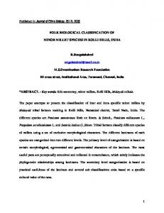
Coming back to the anthropological application we obtained, a OTU character table with 5 lines and 27 columns, applying this coding procedure. This table have been processed by four methods: (1) B method with the H* homogeneity, (2) complete linkage, (3) single linkage and (4) average linkage, the last three with the H* homogeneity particularized to sets with only two OTUs. The best result have been obtained by the B method and haphazard by the complete linkage. It observe only one inversion for the distances in time between any two adjacent periods. (See the Figure 3.)

10


Figure 3. Dendrgram obtained from Manly's Example of Figure 1.

We choose this example because it permit a semantic check of result. In the bottom of the Figure 3 we presented the results of clustering by the three classical methods applied to the famous Mahalanobis's distance. We observe together with Manly that the differences between the five samples can be explained partly as time trends. We said "partly" because probably the most important factor was the migration into the population and this migration do not depend strictly on the dimension of a period.

4.4. A new extension of B Method and a human genetic population application A new fertile idea is to consider the case of a contingency table. For this table we can compute the statistics χ2 for any set of lines (OTUs). We observe that the probability corresponding to this χ2 is an homogeneity. In this way we will obtain a processing of the whole information from table and the possibility of statistical inference on the formed hierarchical clusters.

11


Usually, the classical methods operate with this χ2 for pairs of lines and a lot of authors uses the attached probability for emphasis the significantly clusters, but in our opinion, is not correct. The correct way is our below proposal. A human population genetic application All around of the town Bran, in Brasov aria(in Romania) there are the following six localities: (1) Moeciu de jos, (2) Moeciu de sus, (3) Sohodol, (4) Pestera, (5) Bran, and (6) Simon. An anthropologist (dr. Tatiana Draghicescu from "Victor Babes" Institute, Bucharest, Romania) recorded the sensibility at phenylthiocarbamide (PTC - tasting system) for representative samples from these localities.The results are represented in the contingency table from Table 5. Table 5. The sensibility at phenylthiocarbamide in 6 localities from Romania. T t 405 90 1.MOECIU DE JOS 401 54 2.MOECIU DE SUS 472 75 3.SOHODOL 401 59 4.PESTERA 405 88 5.BRAN 302 12 6.SIMON

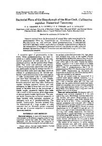
The problem is to cluster these samples in two or more groups which differ significantly. For this reason we propose the B method with probability corresponding to χ2 in a contingency table. We obtain the result from Figure 4.

2). Figure 4. Dendrogram obtained from data of Table 5 by B method applied to p(χ

12


It can observe that sample from Simon high significantly differ of the other ones. On the other hand, there are three groups of samples which significantly differ: , (I) from Bran and Moeciu de jos, (II) from Pestera, Sohodol and Moeciu de sus, and (III) from Simon. The second group have the propriety of homogeneity at the 0.69 level of probability and not exist the properly subgroups more homogenous as this group formed from tree OTUs. If we use a classic method, for example as the single linkage cluster analysis we will obtain the result from Figure 5.

2 Figure 5. Dendrogram obtained from data of Table 5 by Single Linkage applied to p(χ ).

The results from Figure 5 is not correct because the merging of the first group formed from Bran and Moeciu de jos together to the second group formed from Pestera, Sohodol and Moeciu de sus is made by considering the "connection" only between the two members of these groups namely Bran from the first group respectively, Sohodol from the second one. (These two OTUs are the nearest neighbor.) The score χ2 for this pair of OTUs is 3.36 and the corresponding probability is 0.06, (for 1 degree of freedom; 1 = (2 OTUs - 1) x (2 characters - 1)), hence a non-significantly result.

In contrast, because the method proposed by us consider all the "connections" within the set of the two first groups merged we obtained the value 13.024 for the score χ2, score which correspond at the 0.011 level of the probability for 4 degrees of freedom, 4 = ((5 OTUs-1) x (2 characters - 1)) and hence a significantly result. Moreover, our method produce the simultaneous fusion of the three OTUs from the second group, contrarily the classic methods which produce only mutual fusion, performing thus the artifacts (like the single linkage cluster analysis). 13


The others two classic methods (complete linkage cluster analysis and UPGMA) produce the dendrograms analogous with the correct dendrogram but this result is haphazard obtained.

5. References 1. A. Sneath and R. Sokal, Numerical Taxonomy (San Francisco: Freeman, 1973). 2. M. Buser and C. Baroni-Urbani, A direct non dimensional clustering method for binary data. Biometrics 38, pp. 351-360. 3. L. Legendre and P. Legendre, Ecologie Numerique. Tome 2. (Masson and Les Presses de l"Universite de Quebec, 1979). 4. S. Watanabe, Knowing and Guessing. (New York, John Wiley. 1969). 5. L. Dragomirescu, V. Constantinescu and P. Banarescu, A numerical taxonomy method adequate to the biological thinking. Applications: Watanabe's example and the Achonthobrama Genus (Pisces Cyprinidae). Traveaux du Museum d'Histoire naturelle Grigore Antipa, 27, 243-265. 6. L. Dragomirescu, Some extension of Buser and Baroni-Urbani's clustering method. Biometrical Journal, 29, 1-9. 7. Gh. Enescu, Fundamentele logice ale gandirii (Editura Stiintifica si Enciclopedica, Bucuresti, 1980). 8. B.F.J. Manly, Multivariate statistical methods. A primer. (London, New York, Chapman and Hall, 1986).

14