autoregressive model, SAR(1), a variable is a function of its spatial lag (a ... The
spatial term, Wx, is a way to assess the degree of spatial dependence of x in a .....
GRIFFITH, D.A., J. ARBIA (2006) Effects of negative spatial autocorrelation in ...
Estudios de Economía Aplicada ISSN: 1133-3197
[email protected] Asociación Internacional de Economía Aplicada España
LÓPEZ-HERNÁNDEZ, FERNANDO A .; CHASCO-YRIGOYEN, CORO Time-trend in spatial dependence: specification strategy in the first-order spatial autoregressive model Estudios de Economía Aplicada, vol. 25, núm. 2, agosto, 2007, pp. 631-650 Asociación Internacional de Economía Aplicada Valladolid, España
Available in: http://www.redalyc.org/articulo.oa?id=30113193013
How to cite Complete issue More information about this article Journal's homepage in redalyc.org
Scientific Information System Network of Scientific Journals from Latin America, the Caribbean, Spain and Portugal Non-profit academic project, developed under the open access initiative
E
S T U D I O S
D E
E
C O N O M Í A
A
P L I C A D A
V O L . 25-2,
2007. P Á G S . 631-650
Time-trend in spatial dependence: specification strategy in the first-order spatial autoregressive model LÓPEZ-HERNÁNDEZ, FERNANDO A .(*) AND CHASCO-YRIGOYEN, CORO(**) (*)Departamento de Métodos Cuantitativos e Informáticos, Universidad Politécnica de Cartagena, 30203 Cartagena (Spain). (**)Departamento de Economía Aplicada, Universidad Autónoma de Madrid, 28049 Madrid (Spain). Tfo. FALTA - E-mail: (*)
[email protected]; (**)
[email protected]
ABSTRACT The purpose of this article is to analyze the simultaneity of spatial dependence in the first-order spatial autoregressive model, SAR(1). Spatial dependence can be not only contemporary but also time-lagged in many socio-economic phenomena. In this paper, we use three Moran-based space-time autocorrelation statistics to evaluate if spatial dependence is a synchronic spatial effect. A simulation study and an application on the spatial distribution of three economic variables across Spain and Europe shed some light upon these issues. We show evidence of the capacity of these tests to identify the structure (only contemporary, only time-lagged or both contemporary and time-lagged) of spatial dependence in most cases. Keywords: Space-time dependence, Spatial autoregressive models, Moran’s /.
FALTA TÍTULO EN ESPAÑOL RESUMEN En este artículo, se analiza la instantaneidad de la dependencia espacial en el modelo auto-regresivo espacial de primer orden, SAR(1). Son muchos los fenómenos socioeconómicos, en los que la dependencia espacial puede ser no sólo contemporánea, sino también retardada en el tiempo. Con ayuda de tres estadísticos espacio-temporales basados en el test I de Moran, evaluaremos la instantaneidad del efecto espacial. Además, se demostrará la capacidad de dichos tests para identificar la estructura de dependencia espacial (sólo instantánea, sólo retardada en el tiempo y mixta) tanto mediante la realización de un ejercicio de Monte-Carlo como mediante la aplicación a la distribución espacial de tres variables económicas en España y Europa. Palabras clave: Dependencia espacio-temporal, Modelos espaciales auto-regresivos, / de Moran.
JEL classification: C15, C21, C51 Artículo recibido en Octubre de 2006 y aceptado para su publicación en Abril de 2007. Artículo disponible en versión lectrónica en la página www.revista-eea.net, ref.: -25213. ISSN 1697-5731 (online) – ISSN 1133-3197 (print)
632
Fernando A. López-Hernández and Coro Chasco-Yrigoyen
1 INTRODUCTION The purpose of this article is to analyze the time-trend of spatial dependence in the first-order spatial autoregressive model, SAR(1), making a differentiation between two types of spatial dependence: contemporary or synchronic and non-contemporary or time-lagged. The first type is the consequence of a very quick interaction of the process over the neighboring locations, while the second implies that a shock in a certain location needs some time to extend over its neighborhood. It is not easy to separate both types of spatial dependence but both are present very frequently and should be considered when specifying a spatial autoregressive model. Spatial dependence has usually been defined as a spatial effect, which is related to the spatial interaction existing between geographic locations and takes place in a particular moment of time. In other words, spatial dependence is considered as the contemporary coincidence of value similarity with locational similarity. When spatial interaction, spatial spillovers or spatial hierarchies produce spatial dependence in the endogenous variable of a regression model, the spatial autoregressive model has been frequently mentioned as the solution in the literature (e.g. Florax et al. 2003). Analogous to the Box-Jenkings approach in the time-series analysis, spatial model specifications consider autoregressive processes. Particularly, in the first-order spatial autoregressive model, SAR(1), a variable is a function of its spatial lag (a weighted average of the value of this variable in the neighboring locations) for a same moment of time. However, in most socio-economic phenomena, this coincidence in values-locations is not only an instant coincidence but also (or perhaps only) a final effect of some cause that happened in the past, one that has spread through geographic space during a certain period. In this sense, there are some authors that have considered this pure instantaneity of spatial dependence as problematic (Upton and Fingleton 1985, pp 369), suggesting the introduction of a time-lagged spatial dependence term. Moreover, Cressie (1993, pp 450) proposes a generalization of the STARIMA models presented in Martin and Oeppen (1975), Pfeifer and Deutsch (1980) and Hooper and Hewings (1981), among others, such that they also include not only time-lagged but also “instantaneous spatial dependence”. Recently, there are several contributions in this subject. For example, Elhorst (2001, 2003) presented several single equation models that include a wide range of substantive non-contemporary spatial dependence lags, not only in the endogenous but also in the exogenous variables. Anselin et al. (2005) present a brief taxonomy for panel data models with different kind of spatial dependence structure for the endogenous variable (space, time and space-time), referring to them as pure spacerecursive, time-space recursive, time-space simultaneous and time-space dynamic models. The last contribution in this line has been proposed by Di Giacinto (2006), who generalize the STARIMA models including contemporary spatial effects. Estudios de Economía Aplicada, 2007: 631-650 • Vol. 25-2
TIME-TREND IN SPATIAL DEPENDENCE...
633
Space-time dependence has also been specified in spatial autoregressive models in either theoretical frameworks (Baltagi et al. 2003; Pace et al. 1998, 2000) or panel data applications (Case 1991; Yilmaz et al. 2002; Baltagi and Li 2003; Mobley 2003). In this article, we analyze to what extent spatial dependence is a synchronic effect in the SAR(1) model, allowing for not only horizontal (static) but also spacetime interaction (dynamic). Similarly as in Pace et al. (1998, 2000), it is our aim to identify different components in the spatial lag term, splitting it into contemporary, space-time or both –contemporary and space-time- spatial dependence components. Therefore, we propose the identification and use –if necessary- of the space-time lagged endogenous variable in the SAR(1) model, since it reflects the effects due to spatial interaction as a spatial diffusion phenomena, which is not only “horizontal” – simultaneous – but also time-wise. For this purpose, we present some space-time Moran-based statistics in order to identify the spatial dependence structure in the SAR(1) model. We illustrate the performance of these statistics with a simulation exercise and a real case on several economic variables. The remainder of paper is organized as follows. In the next section, we derive three Moran-based autocorrelation statistics to evaluate the simultaneity of the SAR(1) model. In section 3, we present three different specifications of spatial dependence in this model, as well as the behavior of the identification statistics in each one. In section 4, we present the results of the Monte Carlo exercise and the application. Some summary conclusions and references complete the paper. 2 MORAN SPACE-TIME STATISTICS FOR THE EVALUATION OF SPATIAL DEPENDENCE IN THE FIRST-ORDER SPATIAL AUTOREGRESSIVE MODEL The first-order spatial autoregressive model, SAR(1), or simultaneous model dates back to the work of Whittle (1954). In matrix notation, it takes the form: x= á + ñWx + å
(
å : N 0,ó 2 I n
)
(1)
where x is a n by 1 vector of observations; α is a constant; W is the spatial weight matrix; ρ is the spatial autoregressive coefficient; and ε is a n by 1 vector of random error terms. W is the familiar spatial weight matrix that defines the neighborhood interactions existent in a spatial sample (Cliff and Ord 1981). In this context, the usual row-standardized form of the spatial weights matrix can be used, yielding an interpretation of the spatial lag (Wx) as an “average” of neighboring values. Estudios de Economía Aplicada, 2007: 631-650 • Vol. 25-2
Fernando A. López-Hernández and Coro Chasco-Yrigoyen
634
The spatial term, Wx, is a way to assess the degree of spatial dependence of x in a same moment of time (from now on, it is denoted as Wxt). Nevertheless, in most socioeconomic phenomena, the relationship between xt and Wxt is not only synchronic but also –or perhaps only- a final effect of some cause that happened in the past (Wxt-k;
k = 1, 2,... ). Consequently, before estimating a SAR(1) model, we should identify correctly the form of the spatial effect, Wxt, in this model. In this section, we present some Moran-based statistics that are useful to detect the existence of time-lagged spatial dependence. First, we briefly present the spacetime Moran’s I statistic (STI), which evaluates spatial dependence in two instant of time. Secondly, we present two partial space-time Moran’s functions: the partial time-lagged Moran’s I (PLI) and the partial instant Moran’s I (PII). Our goal is to contribute towards obtaining appropriate indicators to evaluate the temporal structure of spatial dependence in the SAR(1) model. 2.1 Space-time autocorrelation When considering both space-time dimensions, some Moran-based statistics can be defined to analyze the space-time structure of a distribution. This is the case of the space-time Moran’s I (STI), originally proposed by Wartenberg (1985). This instrument is similar to others already proposed in the literature (e.g. Cliff and Ord 1981, pp. 23) or Anselin et al. (2002), which introduce a slight modification in STI with the aim of building a Moran scatterplot for space-time processes. The STI is an extension of Moran’s I. It computes the relationship between the spatial lag, Wxt, at time t and the original variable, x, at time t - k (k is the order of the time lag). Therefore, this statistic quantifies the influence that a change in a spatial variable x, that operated in the past ( t - k ) in an individual location i (xt-k) exerts over its neighborhood at present (Wxt). Hence, it is possible to define it as follows:
STIk =
∑ w (x ∑ (x - x i, j
i
ij
i,t -k
i,t -k
t -k
- xt -k )(x j,t - xt ) )2
∑ (x i
i,t
- xt )2 (2)
... where wij is the corresponding element of W matriz, xi,t (with respect to xi,t-k) is the th i observation of vector x in instant t (with respect to t - k ). Note that for k = 0 , this statistic coincides with the familiar univariate Moran’s I that from now on, we denote as I. The significance of this statistic can be assessed in the usual fashion by means of a randomization (or permutation) approach. In this case, the observed values for one
Estudios de Economía Aplicada, 2007: 631-650 • Vol. 25-2
TIME-TREND IN SPATIAL DEPENDENCE...
635
of the variables are randomly reallocated to locations and the statistic is recomputed for each such random pattern. A space-time Moran’s I function could be considered. It is the result of plotting all the values of the STI statistic, adopted by a variable x in time t, for different time lags k. The first value corresponds to the contemporary case, k = 0 , which is the univariate Moran’s I (I), whereas the other ones are proper space-time Moran’s I coefficients (STIk). This function is a particular case of the “full” space-time autocorrelation function (Pfeifer and Deutsch 1980, Bennett 1979), which is a 3-D plot that includes the correlation coefficients for all the space and time lags of a distribution. In general, as stated before, we consider two generating sources of spatial dependence in space-time processes: (b1) Simultaneous or contemporary spatial dependence constitutes the usual definition of spatial dependence in the literature and it is the consequence of an instant, very rapid, spatial diffusion of a phenomenon in geographic space. It can be connected to or the consequence of a lack of concordance between a spatial observation and the region in which the phenomenon is analyzed. (b2) Time-lagged or non-contemporary spatial dependence is the result of a slower diffusion of a phenomenon towards the surrounding space. This kind of dependence is due to the usual interchange flows existing between neighboring areas, which requires of a certain time to be tested. One of the aims of this article is to show a new range of Moran-based statistics that allow justifying the inclusion of both kind of spatial lags, contemporary (Wxt) and time-lagged (Wxt-k) ones, to explain xt in a spatial regression. Some coefficients can be defined to evaluate the inclusion of a space-time lag term in a spatial regression. The space-time Moran’s I (STI) –equation (2)- it is possible to connect this statistic with the standard Pearson correlation coefficient between these two variables, as also derived by Lee (2001). So we can express the STI statistic as:
STIk = rxt-k ,x%t
∑ (x% ∑ (x i
i,t
- x% t )2
i
i,t
- xt )2
(3)
Where x% t = Wxt y rxt-k ,x%t is the Pearson linear correlation coefficient between xt-k and x%t . 2.2 Partial Moran’s I indexes The basic underlying idea consists of eliminating the influence of one of the dimensions in order to compute separately contemporary and non-contemporary Estudios de Economía Aplicada, 2007: 631-650 • Vol. 25-2
Fernando A. López-Hernández and Coro Chasco-Yrigoyen
636
spatial dependence. For this purpose, we substitute in (3) the space-time correlation coefficient by a partial correlation one. Two space-time partial autocorrelation statistics can be defined: (a) Partial Time-Lagged Moran’s I (PLI) computes the correlation between variable x in period t-k and its spatial lag Wx in period t removing the influence of x in t: PLIk = Corr( xt -k , x% t xt )
Corr( xt -k , x% t xt ) =
∑ (x% ∑ (x i
i,t
- x% t )2
i
i,t
- xt )2
;
k = 1,2,...,t -1 (4)
rxt-k ,x%t - rxt-k ,xt ⋅ rx%t ,xt 1- rx2
,x
⋅ 1- rx%2 ,x
t-k t t t where is the partial correlation coefficient of variables xt-k and Wxt after eliminating the correlation from xt. Therefore, it is possible to express this statistic as a function of both Moran’s I and space-time Moran’s I:
PLIk =
STIk - rxt-k ,xt ⋅ I 1 - rx2t-k ,xt ⋅ 1 - rx2t ,x%t
(5)
This indicator removes contemporary spatial dependence from the relationship between variables xt-k and Wxt. If the pattern of spatial dependence is one that can be totally captured by contemporary spatial dependence ( I ≠ 0 ), then the PLI will be close to zero. On the contrary, if the process is one that can be captured by noncontemporary spatial dependence, then PLIk will be significantly different from zero. Regarding to the sign, it is positive/negative depending on STIk sign. (b) Partial Instant Moran’s I (PII) is the complementary expression that consists of computing contemporary –or instant- spatial dependence after removing time-lagged spatial dependence by means of an index: t
PIIk = Corr( xt , x% t xt -k )
∑ (x% ∑ (x i
i,t
- x% t )2
i
i,t
- xt )2
; k = 1,2,...,t -1 (6)
where Corr( xt , x% t xt -k ) is the partial correlation coefficient of variables xt and x%t after eliminating the correlation from xt-k. Therefore, it is possible to express this statistic as a function of both Moran’s I (It) and space-time Moran’s I (STIk).
Estudios de Economía Aplicada, 2007: 631-650 • Vol. 25-2
TIME-TREND IN SPATIAL DEPENDENCE...
637
PIIk =
I - rxt-k ,xt ⋅ STIk 2
1 - rxt -k ,xt
⋅ 1 - rx%2 ,x t
t -k
(7)
This indicator removes time-lagged spatial dependence from the contemporary spatial relationship between variables xt and x%t . If the pattern of spatial dependence is one that can be totally captured by a time-lagged spatial autoregression, then the PII will be close to zero. On the contrary, if the process is one that can be captured by contemporary spatial dependence, then PII will be significantly different from zero. From (5) and (7), it is easy to derive the following expression:
I=
1 - rx%2t ,xt-k 1- r
2 xt-k ,xt
PIIk +
1 - rx%2 ,x ·rx t
1- r
t
t -k
2 xt-k ,xt
,xt
PLIk ; k = 1, ...,t -1 (8)
In this expression, spatial dependence (measured with Moran’s I statistic) is shown as the sum of two contributions: contemporary spatial dependence (PII) and noncontemporary spatial dependence (PLI), both weighted by a corresponding scalar. Next, we tackle a double exercise with the aim of evaluating the utility of these indicators. Firstly, we build a Monte Carlo experiment to analyze how they react to different situations. Secondly, we apply the indexes to the analysis of spatial dependence in the distribution of several variables in Spain and Europe. 3. SOME EVIDENCE IN THE PERFORMANCE OF PARTIAL MORAN INDEXES. 3.1 Monte Carlo simulation study In this subchapter, we evaluate empirically the Moran space-time autocorrelation statistics (I, STI, PLI, PII) in a series of Monte Carlo simulation in order to obtain an initial assessment of their discriminating power of spatial dependence into contemporary and/or time-lagged. 3.1.1. Experimental design We consider two different moments of time t, s, such that s < t . For time s, we generate an instant spatial dependence process (xs) whereas for time t we set up three alternative processes (xt): instant spatial dependence (i), time-lagged spatial dependence (ii) and both instant and time-lagged spatial dependence (iii). Formally: Estudios de Economía Aplicada, 2007: 631-650 • Vol. 25-2
Fernando A. López-Hernández and Coro Chasco-Yrigoyen
638
i)
For time t, instant spatial dependence only: xs = á + ñWx + ås s xt = á + ñWx + åt t
ii)
s
(9)
t
For time t, time-lagged spatial dependence only: xs = á + ñWx + ås s xt = á + ñWx + ås t
s
(10)
t
iii) For time t, both instant and time-lagged spatial dependence: xs = á + ñWx + ås s
s
xt = á + ñtWx 1 + ñt Wx 2 + ås
t
(11)
where αs and αt are constant terms, ρ, ρ1, ρ2 are the spatial autoregressive coefficients and εs, εt are the error terms for time s, t, respectively. In this experiment, we use five different spatial weight matrices in order to capture diverse spatial configurations. They allow showing an ample set of possible results, in terms of area size (100, 259 and 400 spatial units) and connectivity association. Thus, two matrices (w10r, w10q) are defined on a 10 ×10 regular square lattice ( N = 100 ) using the rook and queen criterion, respectively (Anselin 1988, p. 18). Two other matrices (w20r, w20q) are defined in the same fashion though on a 20 × 20 regular square lattice ( N = 400 ). Finally, we also consider another matrix (wue) on the surface corresponding to the EU-27 nuts II division (259 regions). In this case, wij is calculated as the squared inverse distance between each region centroids. All the matrices are row-standardized. Clearly, we can obtain different degrees of instant and time-lagged spatial dependence by manipulating the values of the parameters and the characteristics of the error terms. In our experiments, we set the purely temporal dependence structure in variable x by means of the error terms (εs, εt), which are generated as a bivariate normal
( )
distribution with zero mean and Σ = σ ij covariance matrix, such that σ ii = 1 and
σ ij = r . Temporal autocorrelation is defined by the r parameter considering three different cases: weak temporal autocorrelation ( r = 0.5 ), moderate temporal autocorrelation ( r = 0.75 ) and strong temporal autocorrelation r = 0.95 ).
Estudios de Economía Aplicada, 2007: 631-650 • Vol. 25-2
TIME-TREND IN SPATIAL DEPENDENCE...
639
In the case of expression (11) –both instant and time-lagged spatial dependence in time t, we also consider two different intensities in spatial dependence: (11.a) Stronger instant spatial dependence: ñ1 = 2ñ2 and ñ1 + ñ2 = ñ . (11.b) Stronger time-lagged spatial dependence: 2 ñ 1= ñ
2
and
ñ + ñ 2= ñ . 1
Therefore, we compute the space-time partial autocorrelation statistics in time t, with respect to time s, for the different values of parameters r, ρ. We have only considered a positive spatial autocorrelation structure, which is the most common tendency found in empirical cases (Griffith and Arbia 2006). In the simulations, we let ρ vary from zero to one, with increments of 0.05, to assess the effect of spatial lag autocorrelation (the value ñ = 0 is substituted by 0.995 to avoid indetermination problems). We have generated 9,999 replications for each situation. We have evaluated the power of the test statistics (I, STI, PLI, PII) to discriminate between contemporary, time-lagged or both kind of spatial dependence structure in the SAR(1) model. 3.1.2. Results Figures 1-4, present the simulation results. In each chart, we have represented in columns the different spatial configurations (5 spatial weight matrices). The first three rows show temporal dependence values ( r = 0.5, 0.75 and 0.95). Each graph let us see the mean values of the four indexes I, STI, PII, PLI (in vertical axis) for different degrees of spatial dependence ρ (in horizontal axis). The fourth row is reserved to illustrate the number of times, in percentages, P II > P LI (with respect to P LI > P II ), when the process has been generated following the structure shown in (9) and (11. a), with respect to (10) and (11.b). This percentage is a good indicator to evaluate the utility of the partial indexes to discriminate between different situations. In general, the results highlight the following results: 1. The four indexes exhibit a significant differential behavior when evaluating different Data Generating Processes (DGP). 2. The mean value of these indexes is quite similar, with small differences independently of the spatial structure and connectivity degree in the data. 3. The higher the temporal correlation is, the lower the indicators capacity to discriminate between different processes. Figure 1 shows the results of the (9) DGP, where spatial dependence is contemporary in both periods. In this case, the Moran I and STI indexes display very similar values, being the first slightly higher, in average, than the second. On the contrary, the partial indexes have a dissimilar behavior: the mean value of PLI is always close to zero whereas the mean value of PII tends to increase with ρ. If we compare these results with those in Figure 2, which represents a DGP with time-lagged spatial lag Estudios de Economía Aplicada, 2007: 631-650 • Vol. 25-2
640
Fernando A. López-Hernández and Coro Chasco-Yrigoyen
dependence (expression 10), we can observe that I and STI have a similar performance than in Figure 1, though STI is now slightly higher, in average, than Moran’s I. In summary, the two global indexes have no discriminating capacity between contemporary and time-lag spatial dependence while the partial ones do it quite well. In effect, the percentage of times PII > PLI in process (9), with respect to PLI > PII in process (10), increases with spatial dependence (ρ) and decreases with temporal dependence (r). There are also variations in partial indexes when considering different surface sizes and/or connectivity degrees in W matrix. The percentage of expected results is higher with surface size and the rook contiguity criterion (with respect to the queen). Figures 3 and 4 show the results for the mixed DGP (11.a) and (11.b). In these two situations, indexes performance is worse due to the inherent difficulties to split into two very similar processes. Moran’s I and STI are very similar -almost identical- in average. Indeed, evidence is much weaker in the case of the partial indexes. Specifically, when temporal dependence is stronger in mixed processes (Figure 3), both partial indexes are equal in average, though when ρ is close to one, the mean PLI values are higher than PII, as expected. When spatial dependence is generated as in expression (11.a) -stronger simultaneous dependence- the partial indexes performs better, particularly when ρ and sample sizes are higher. In these cases, the percentage of times that PII > PLI is over 90%. 3.2 Empirical application In this subchapter, we show the performance of the different Moran’s I (I, STI, PII, PLI) when applied to three spatially autocorrelated economic variables1: GDP, ADSL and foreign residents. • “GDP” is the Europe Per Capita GDP in Purchasing Power Standards (PPS) provided by Eurostat. The data is available for the period 1999-2004 and 259 European regions (nuts II) corresponding to 27 countries. • “Broadband lines” is the number of DSL telephone lines provided by Telefonica S.A. The data is available for the period 1999-2004 and the 179 municipalities of the Region of Madrid (nuts V). • “Foreign residents” is the number of residents born abroad as a proportion of total population. This variable is available in the Padrón de Habitantes of the Spanish Office for Statistics (INE). The data is available for the period 1999-2004 and 50 Spanish provinces (nuts III).
1 Other applications for Spanish series can been analyzed in Chasco and López 2007 Estudios de Economía Aplicada, 2007: 631-650 • Vol. 25-2
TIME-TREND IN SPATIAL DEPENDENCE...
641
If we take 2004 as a reference year, we can analyze the evolution of the partial Moran’ I when relating the values of a variable between this reference and the years before (1999-2003). We can also compare -as a confirmatory analysis- the partial indexes with the significance of the estimates ρs and ρ2004 in the following model: x 2004 = á + ñ2004Wx 2004 + ñ2004 Wx +så
s
2004
s =1999,..., , 2003
(12)
being W a spatial weight matrix, in which each element (wij) is set to one if two spatial units (either EU or Spanish regions and municipalities) share a common border and zero otherwise. Thus, we expect a significant ρ2004 parameter in variables with predominant contemporary spatial dependence. In these cases, P II > P LI as demonstrated in the Monte Carlo exercise (Figure 1). On the other side, the ρs parameter in equation (12) will be significant when P LI > P II (Figure 2), that is to say, for a leading time-lagged spatial dependence. All the variables exhibit strong temporal autocorrelation, as shown in Table 1. In the case of per capita GDP and Foreign resident (FR), we obtain a Pearson coefficient above 0.99 and 0.84, respectively, between the spatial series in the year 2004 and the previous ones. Regarding DSL, it is the least temporally autocorrelated variable, with an increasing correlation coefficient from 0.71 (provincial series in 1999 and 2004), to 0.96 (provincial series in 2003 and 2004). In Figure 5, we have illustrated the Moran’s I indexes for these variables. GDP has high STI and PLI values, quite above PII for all the time-lags, which highlights the existence of persistent time-lagged spatial dependence in this variable. This is confirmed by the estimation results of model (12), as seen in Table 2. When regressing regional GDP in 2004 on its spatial lag referred to different s periods ( s = 1999, ..., 2003 ), the results exhibit a non-significant contemporary spatial dependence term (Wx2004) in presence of the corresponding space-time lagged term (Wxs). From an economic point of view, this conclusion confirms the fact that spatial diffusion in GDP is a long-term process. That is to say, changes in EU-regional GDP take some time to spread to other neighboring regions. The second case, municipal “broadband lines” in 2004 (DSL), displays a different situation: though STI values are fairly high, P II > P LI in all periods, except for s = 2003 . The partial coefficients point out the existence of significant contemporary spatial dependence, which is corroborated by the confirmatory analysis (Table 2). All the regressions of DSL in 2004 on its contemporary and non-contemporary spatial lags exhibit very significant coefficients, pointing out the existence of mixed (contemporary and time-lagged) spatial dependence. This is probably due to the nature of this innovative variable, which has experienced a striking rising during the last
Estudios de Economía Aplicada, 2007: 631-650 • Vol. 25-2
642
Fernando A. López-Hernández and Coro Chasco-Yrigoyen
years, particularly in Madrid. That is to say, an increase in DSL lines in a municipality has two effects: part of it has a quick diffusion over the neighboring municipalities, though another fraction needs some time to extend over its neighborhood. There is also another reason for mixed spatial dependence in this variable, e.g. the lower spatial disaggregation of the sample (nuts V). In effect, contemporary spatial dependence could also be due to a lack of correspondence between the observed data at the level of municipalities (nuts V) and the real spatial scale of this phenomenon, which comprises a set of near municipalities (nuts IV). The last example corresponds to provincial “foreign residents” in 2004 (FR). As shown in Figure 5 (third row), STI coefficient is quite high though PII > PLI , which is the same situation as DSL. Nevertheless, in this case, STI values -which are usually quite elevated- become appreciably lower (below 0.3) from 2001 to the past. This is an evidence of a noteworthy non-contemporary spatial dependence only during the first time lags. This is what takes place in the confirmatory analysis, in which Wxs is only significant for the first 3 periods (2003, 2002, 2001). In summary, “foreign residents” is also an instance of non-contemporary spatial dependence, as GDP, though in this case, diffusion is much quicker (only 2 or 3 years) from one spatial unit (provinces) to another. In effect, foreign residents have experienced a prominent raise in Spain (mainly in certain areas) during the last years. This is why an increase of this variable in a province (nuts III) has a rapid response in neighboring provinces, though it lasts 1, 2 or 3 years to be completed. 4. CONCLUSIONS The main aim of this paper is the analysis of the instantaneity of spatial dependence in the SAR(1) model, making a differentiation between instant or contemporaneous and lagged or non-contemporaneous spatial dependence. The first is the consequence of a very quick diffusion of the process over the neighboring locations, while the second implies that a shock in a certain location needs of several periods to take place and be tested over its neighborhood. It is –without any doubt- a subject to consider when working with space-time distributions, though it is not easy to differentiate between both kinds of dependencies, especially when dealing with highly correlated time-series. For the fulfillment of this aim, we propose the use of Moran’s I joint with three Moran’s I-based statistics: space-time Moran’s I (I), partial instant Moran’s I (PII) and partial time-lagged Moran’s I (PLI). We illustrate the performance of these tests for the identification of spatial dependence structure via a simulation exercise and a real-life application. In the simulation experiment, we build three data generating processes based on different spatial dependence structures: only contemporary, only time-lagged and both contemporary and time-lagged. Estudios de Economía Aplicada, 2007: 631-650 • Vol. 25-2
TIME-TREND IN SPATIAL DEPENDENCE...
643
In the primary two cases, this experiment has clearly revealed the good performance of the Moran’s tests, mainly in processes with strong spatial autocorrelation (instant and/or time-lagged) and weaker temporal correlation. Nevertheless, in the extreme case of (nearly) null spatial autocorrelation and (nearly) perfect temporal correlation, it is very difficult to split both kind of spatial dependence, since there is a practical identification between the process in both –past and present- periods. Regarding the mixed spatial dependence, the space-time Moran’s tests are less efficient in general. Only in the case of extreme spatial autocorrelation and weak temporal correlation, the performance of these statistics is acceptable in order to split spatial dependence into instant and time-lagged. Finally, we have used these indexes with the aim of identified the nature of spatial dependence in various socioeconomic phenomena at different spatial scales. In the three proposed cases, the Moran’s I indexes performance is coherent with the empirical results obtained from a confirmatory analysis. 5. REFERENCES ANSELIN, L. (1988) Spatial econometrics: methods and models (Boston, Kluwer Academic Publishers) ANSELIN, L, J. LE GALLO & H. JAYET (2006) Spatial panel econometrics, in: Matyas L & P. Sevestre (eds) The econometrics of panel data (Boston, Kluwer Academic Publishers) ANSELIN, L, I. SYABRI & O. SMIRNOV (2002) Visualizing multivariate spatial correlation with dynamically linked windows, in: Anselin L & S. Rey (eds) New tools in spatial data analysis. Proceedings of a workshop, Center for Spatially Integrated Social Science, University of California, Santa Barbara, CDROM BALTAGI, B.H. & D. LI (2003) Prediction in the panel data model with spatial correlation, in: Anselin L, R. Florax & S. Rey (eds) New Advances in Spatial Econometrics (Berlin, Heidelberg, New York, Springer) BALTAGI, B.H., S.H. SONG & W. KOH (2003) Testing panel data regression models with spatial error correlation, Journal of Econometrics, 117-1, pp. 123-150 BENNETT, R.J. (1979) Spatial time series: forecasting and control (London, Pion) CASE, A. (1991) Spatial patterns in household demand. Econometrica, 59, pp. 953–965 CRESSIE, N. (1993) Statistics for Spatial Data (New York, Wiley) CLIFF, A. & ORD, J. (1981) Spatial processes, models and applications. (London, Pion) CHASCO, C. AND F.A. LÓPEZ (2007) Is spatial dependence an instantaneous effect? Some evidence in economic series of Spanish provinces. Estadística Española. Forthcoming.
Estudios de Economía Aplicada, 2007: 631-650 • Vol. 25-2
644
Fernando A. López-Hernández and Coro Chasco-Yrigoyen
DI GIACINTO V. (2006) A generalized space-time ARMA model with an application to regional unemployment analysis in Italy, International Regional Science Review, 29, pp. 159-198. ELHORST, J.P. (2001) Dynamic models in space and time, Geographical Analysis, 33, pp. 119-140. ELHORST, J.P. (2003). Specification and estimation of spatial panel data models, International Regional Science Review, 26(3), pp. 244–268 FLORAX, R., H. FOLMER & S. REY (2003) Specification searches in spatial econometrics: the relevance of Hendry’s methodology, Regional Science and Urban Economics, 33, pp. 557-579 GRIFFITH, D.A., J. ARBIA (2006) Effects of negative spatial autocorrelation in regression modeling of georeferenced random variables. I Workshop in Spatial Econometrics, Rome, 25-27 2006 HOOPER, P., G.J.D. HEWINGS (1981) Some properties of space-time processes, Geographical Analysis, 13, pp. 203-223. LEE, S-I (2001) Developing a bivariate spatial association measure: an integration of Pearson’s r and Moran’s I, Journal of Geographical Systems, 3, pp. 369-385 MARTIN, R.L., J.E. OEPPEN (1975) The identification of regional forecasting models using space: time correlation functions, Transactions of the Institute of British Geographers, 66, pp. 95-118 MOBLEY, L.R. (2003) Estimating hospital market pricing: an equilibrium approach using spatial econometrics, Regional Science and Urban Economics, 33, pp. 489–516 PACE, R.K., R. BARRY, J.M. CLAPP & M. RODRÍGUEZ (1998) Spatiotemporal autoregressive models of neighborhood effects, Journal of Real State Finance and Economics, 17(1), pp. 15-33 PACE, R.K., R. BARRY, O.W. GILLEY & C.F. SIRMANS (2000) A method for spatial-temporal forecasting with an application to real estate prices, International. Journal of Forecasting, 16, PP. 229-246 PFEIFER, P.E. & S.J. DEUTSCH (1980) Identification and interpretation of first-order space-time ARMA MODELS,TECHNOMETRICS, 22(3), PP. 397-403 UPTON, G. & B. FINGLETON (1985) Spatial data analysis by example: volume 1 point pattern and quantitative data (New York, Wiley) WARTENBERG D. (1985). Multivariate spatial correlation: A method for exploratory geographical analysis, Geographical Analysis, 17: 263–283. WHITTLE, P. (1954) On stationary processes in the plane, Biometrika, 41, pp. 434-449 YILMAZ, S., K.E. HAYNES & M. DINC (2002) Geographic and network neighbors: spillonver effects of telecommunications infrastructure, Journal of Regional Science, 42-2, pp. 339-360.
Estudios de Economía Aplicada, 2007: 631-650 • Vol. 25-2
TIME-TREND IN SPATIAL DEPENDENCE...
Estudios de Economía Aplicada, 2007: 631-650 • Vol. 25-2
645
646
Fernando A. López-Hernández and Coro Chasco-Yrigoyen
Estudios de Economía Aplicada, 2007: 631-650 • Vol. 25-2
TIME-TREND IN SPATIAL DEPENDENCE...
Estudios de Economía Aplicada, 2007: 631-650 • Vol. 25-2
647
648
Fernando A. López-Hernández and Coro Chasco-Yrigoyen
Estudios de Economía Aplicada, 2007: 631-650 • Vol. 25-2
TIME-TREND IN SPATIAL DEPENDENCE...
649
Figure 5: Moran’s I indexes and coefficient p-values of variables GDP, HP and IPC. Moran’s I indexes 0.5 0.4
GDP
0.3 0.2 0.1 0.0 1998
1999
2000
2001
I Moran
STI
2000
2001
I Moran
STI
2002
2003
2004
2003
2004
2003
2004
-0.1
PII
PLI
0.6 0.5
DSL
0.4 0.3 0.2 0.1 0.0 1998
1999
2002
PII
PLI
0.5 0.4 0.3 0.2
FR
0.1 0.0 1998 -0.1
1999
2000
2001
I Moran
STI
2002
-0.2 -0.3 -0.4
Estudios de Economía Aplicada, 2007: 631-650 • Vol. 25-2
PII
PLI
Fernando A. López-Hernández and Coro Chasco-Yrigoyen
650
Table 1: Temporal correlation of the variables in 2004 and past periods. GDP DSL FR
2004
2003
2002
2001
2000
1999
1,000 1,000 1,000
0,999 0.960 0.997
0,994 0.906 0.952
0,988 0.852 0.910
0,985 0.774 0.881
0,977 0.712 0.841
Table 2: Estimation results of equation (12) for variables GDP, ADSL, FR. Variable 2003
2002
2001
2000
1999
Coeff.
GDP p-value
Coeff.
DSL p-value
Coeff.
FR p-value
Wxs
1.13*
0.000
1.14*
0.000
0.85*
0.000
Wx2004
-0.04
0.761
0.04
0.698
0.08
0.627
Wxs
1.08*
0.000
1.10*
0.000
0.91*
0.001
Wx2004
0.00
0.983
0.31*
0.001
0.19
0.265
Wxs
1.16*
0.000
1.71*
0.000
0.83*
0.025
Wx2004
-0.04
0.759
0.33*
0.000
0.33*
0.037
Wxs
1.20*
0.000
2.78*
0.000
0.59
0.197
Wx2004
-0.04
0.765
0.43*
0.000
0.45*
0.003
Wxs
1.32*
0.000
4.39*
0.000
0.50
0.354
Wx2004
-0.05
0.708
0.49*
0.000
0.48*
0.001
Notes: We have omitted the constant values. (* *) p-values above 0.05.
Estudios de Economía Aplicada, 2007: 631-650 • Vol. 25-2