Detected signals are horizontal and vertical interference fringe intensities, which are modulated double side band signa
1 of 4
Speckle Noise Reduction and Segmentation on Polarization Sensitive Optical Coherence Tomography Images Hyohoon Choi, Thomas E. Milner, Alan C. Bovik University of Texas at Austin, TX, USA Abstract— The retinal layers of a monkey were imaged using a Polarization Sensitive Optical Coherence Tomography (PS-OCT) system in an effort to develop a clinically reliable automatic diagnostic system for glaucoma. Glaucoma is characterized by the progressive loss of ganglion cells and axons in the retinal nerve fiber layer (RNFL). Automatic segmentation of the RNFL from the PS-OCT images is a fundamental step to diagnose the progress of the disease. Due to the use of a coherent light, speckle noise is inherent in the images. Wavelet denoising techniques with a combination of image processing techniques were applied to remove the speckle noise in the PS-OCT images, and a fuzzy logic classifier was used to segment the RNFL. A significant signal to noise ratio improvement was observed qualitatively and quantitatively after the denoising. The upper boundary for the RNFL was reliably detected, but the lower boundary detection still remains as a problem. Keywords—PS-OCT, speckle noise, wavelet denoising, glaucoma
I. INTRODUCTION Glaucoma is a serious ocular disease ranking as the second leading cause of blindness worldwide [1]. Glaucoma is characterized by the progressive loss of ganglion cells and axons in the RNFL. If not detected in the early stage, glaucoma can result in partial or total blindness. Clinically, the disease results initially in peripheral and subsequently central vision loss. Some evidence indicates that thinning of the nerve fiber layer can occur up to 6 years prior to clinically detectable vision loss. Thus the thickness of the RNFL reduces and the amount of phase retardation decreases with the progression of glaucoma. Unfortunately early diagnosis of glaucoma with high specificity and sensitivity using standard clinical diagnostic instrumentation remains problematic. There are several clinical techniques for retinal examination including red-free photography, confocal laser scanning tomography (SCLT), optical coherence tomography (OCT), and scanning laser polarimetry (SLP). Red-free photography is used at a few larger centers, but the technique is far too labor intensive, and moreover this technique is fundamentally limited because the analysis is subjective and dependent on the physician. SCLT has limited longitudinal resolution due to the low numerical aperture of the human eye. The two primary competing technologies for quantitative RNFL analysis are optical coherence tomography (OCT) and scanning laser polarimetry (SLP). OCT has emerged as a
promising technique for high-resolution cross-sectional imaging of biological samples such as the retinal nerve fiber layer. Several studies show that OCT could be effectively used to detect quantitative differences in RNFL thickness. In SLP the patient’s eye is illuminated with polarization modulated laser light focused onto the retina. Specificity and sensitivity of SLP for detecting glaucoma are not high enough to render this technique useful in clinical practice. A. PS-OCT PS-OCT is similar to OCT with the polarization state of light controlled in the interferometer source, sample and reference paths. PS-OCT combines the advantages of OCT to measure retinal nerve fiber layer (RNFL) thickness and scanning laser polarimetry to determine RNFL phase retardation. PS-OCT technique can provide maps of both RNFL thickness and phase retardation per unit depth (PR/UD) [4]. Detected signals are horizontal and vertical interference fringe intensities, which are modulated double side band signals. Since polarization information in light backscattered from the sample is encoded in the amplitude and phase of horizontal and vertical interference fringe intensities, processing of the corresponding complex analytic signals ( Γ% h and Γ% v ) is convenient. Γ% h and Γ% v are determined by coherently demodulating horizontal and vertical interference fringe intensities. For each scan line, PS-OCT provides demodulated horizontal and vertical fringe amplitudes ( Γ% and Γ% ) and their relative phase h
difference ( φv , h
v
= ∠Γ% v − ∠Γ% h ). They are functions of
position on a scan line (A-scan line). By taking the sequence of A-scan lines (B-scan), PS-OCT provides a twodimensional cross sectional image. B. Speckle noise Speckle arises as a natural consequence of the limited spatial-frequency bandwidth of the interference signals measured in OCT [3]. In images of highly scattering biological tissues, speckle has a dual role as a source of noise and as a carrier of information about tissue microstructure. Thus the speckle is both a source of noise in OCT and the signal itself. In the context of optical coherence tomography, the objective of speckle reduction is to suppress signal-degrading speckle and accentuate signalcarrying speckle. Among the most popular image processing methods for speckle reduction are median filtering, homomorphic Weiner filtering, multiresolution wavelet analysis, adaptive smoothing, and anisotropic diffusion [5].
2 of 4 All of these methods incorporate either an explicit or implicit statistical model of the spatial frequency spectra of the target features and background. Since the power spectral densities of the signal-carrying and signal-degrading speckle overlap, some loss of useful information is inevitable. In recent years, wavelet techniques have been successfully employed in speckle noise reduction for medical ultrasound, SAR, and OCT images by employing a non-linear thresholding on wavelet coefficients [2]. The rest of the paper describes methods to remove the speckle noise on horizontal, vertical, and phase-difference magnitude images by wavelet soft thresholding and other image processing techniques. Pixel classification by fuzzy logic classifier to detect the RNFL was performed utilizing horizontal, vertical, and phase-difference information after removing the speckle noise. Their results are presented in the result and appendix. II. METHODOLOGY Once the demodulated fringe amplitude signals are calculated, signals are stored as 32 bit data in a size of 300 by 11704 images. Number 300 corresponds to 300 A-scan lines. A. Wavelet denoising When a noisy signal is represented in the wavelet domain, large coefficients tend to be associated with the main structure of the signal whereas smaller coefficients are mainly related to noise. The main idea behind wavelet domain denoising is that the signal to noise ratio can be improved by suppressing the small coefficients and by enhancing the large coefficients. The manipulation of the coefficients can be done by hard thresholding or soft thresholding. In hard thresholding algorithms, coefficients smaller than an absolute threshold are eliminated. Instead of simply eliminating coefficients smaller than the threshold, in the soft thresholding, a nonlinear function is used to suppress smaller coefficients. In wavelet denoising, the signal is assumed to be corrupted by the additive white noise. Speckle noise is known to be a multiplicative noise; the multiplicative noise becomes additive noise by taking logarithm on the image. J. M. Schmitt et al. have successfully used wavelet denoising to reduce the speckle noise on OCT images [2]. They found that, on average, the magnitude of the image signal to noise ratio (SNR) can be improved about 10 times and the contrast to noise ratio (CNR) about 1.5 times. The SNR was defined as µ (1) SN R= σ where µ and σ are the mean and standard deviation of the pixel magnitudes in a ROI in the image. The SNR quantifies the relative magnitudes of the signal and noise powers. The CNR was defined as
CNR =
µn − µr
(2)
δ n2 + δ r2
µn and µr are the means computed for the target and reference areas, respectively, and δ n and δ r are the where
corresponding standard deviations. The CNR is generally a more robust measure of image quality because it incorporates a measure of contrast (the difference of means) that does not increase without bound as the image becomes smoother. The target and reference area are shown in Fig. 2. In our case, denoising of the horizontal and vertical magnitude images was performed on each A-scan line instead of performing 2D wavelet denoising on a whole image. 5 levels of decomposition were performed and a soft thresholding called ‘Heursure’ in Matlab program was applied. The speckle noise removal process for horizontal and vertical magnitude images are identical. Phasedifference magnitude images have different types of noise than white noise as shown in Fig. 3 and 4 (b). Thus, direct application of wavelet denoising would not work. For phasedifference magnitude images, first a 3-tap Laplacian, (-1 2 – 1), filtering was performed on each A-scan. A Laplacian filtered signal oscillates about zero with variances proportional to the signal frequencies (Fig. 4(a)). Values with large variances correspond to the noise we want to eliminate. Those values are easily found by a simple thresholding, e.g. S is the noise when |S| > t, t = σ where S is the Laplacian filtered signal, t is the threshold and σ is the variance of S. After removing those values from the signal (Fig. 4 (b)), tophat filtering was performed on the entire image with a 5 by 5 window to eliminate impulse noise (Fig. 4 (c)): Tophat = Im – open(Im)
(3)
Subtracting Fig. 4(c) from Fig. 4(b), Fig. 4(d) was obtained which then further denoised by wavelet denoising with soft thresholding. B. Image segmentation Once the noise has been removed, the segmentation of the region of interest becomes easier. However a simple thresholding or an adaptive thresholding does not work in our case. A RGB image is created assigning horizontal magnitude as red channel, vertical magnitude as green channel, and phase-difference image as blue channel. Luminance information of the RGB image was used to detect the upper boundary. Since the transition between the background and the RNFL is significant, and RNFL is the first layer encountered from the background, a simple threshold applied to the luminance image gives a region with a clear upper boundary of RNFL as shown in Fig. 6 (left). A fuzzy logic classifier was used to classify the pixels based on the pixel intensity values of the three channels. As shown in Fig. 5, three magnitude values are used as features
3 of 4 for the classifier and two classes were assumed, one for the retina layer and one for the other layers. An important assumption was made for using horizontal, vertical and phase-difference magnitudes as features. The assumption is that depending on the tissue section, the combination of three magnitudes will be similar in the same tissue and different between different tissues. Pixel values were regarded as probability density values, and it was further assumed that each feature is independent on each other. Then the posterior probability that having a class c given three pixel values can be found as P(wc | h, v, p) = h(i, j) ⋅ v(i, j) ⋅ p(i, j)
c = 1,2
i, j = 1~ N
(4)
where wc is the class, h(i,j), v(i,j), p(i,j) are the normalized pixel values at location i,j. A pixel at (i, j) belongs to class 1 when P ( w 1 | h , v , p ) > P ( w 2 | h , v , p ) and vice versa. Background pixels are easily found since the posterior probability for the background is zero because p(i,j) is zero on the background. Knowing that the RNFL is the top layer, and having the upper boundary information, post-processing on the classification result removed all of the misclassified pixels that were not connected to the top layer. Labeled samples (ground truth) were manually selected from an RGB image, and a randomly selected half of the data was used for the training, and all of the samples were used for the testing. III. RESULTS Fig. 1 (left) is the original horizontal magnitude image, and Fig. 1 (right) shows the denoised image. Noise has been effectively removed as shown in Fig. 1 (right). Fig. 2 is a profile of Fig. 1 at row = 100. A little graph on the left upper corner on Fig. 2 is a close up of the signal where only noise is present from column 1000 to 2000, which illustrates that noise variance has been reduced significantly after the wavelet denoising. Fig. 4 shows the process of noiseremoval for phase-difference magnitude images. As shown in Fig. 4 (a), places where the actual signals are located have low magnitude, thus simple thresholding could find the locations of the noise as explained earlier. Fig. 4 (b) shows the image after the noise was removed from the original image. It still contains a lot of noise. Tophat filtering with a small size of window (5 by 5) was used to pick up those white spots, and Fig. 4 (c) shows the white spots found by Tophat filtering. Then Fig. 4 (c) was subtracted from Fig. 4 (b), and Fig. 4 (d) is the result. This denoised signal was further denoised using wavelet denoising with soft thresholding. The resultant signals are shown in Fig. 3 (right) and Fig. 5. The noise has been effectively removed. As shown in Table 1 and 2, SNR improvement after the denoising is about 2 times, and CNR improvement is about 9 percent. Significant SNR improvement was achieved from
where noise was dominant (Area 1), and less SNR improvement was observed where the signal (tissue, Area 2) was present. All the areas in Table 1 and 2 are shown in Fig. 2. The result of fuzzy logic classifier is shown in Fig. 6 (right). Only the boundary is displayed on Fig. 6 by subtracting the erosion of detected RNFL region from the detected RNFL region. Table 1. SNR comparisons SNR Original Denoised Ratio
Horizontal Area 1 Area 2 1.7303 1.9430 4.4961 2.0609 2.5985 1.0607
Vertical Area 1 Area 2 1.8561 1.7692 5.1150 1.9477 2.7557 1.1009
Table 2.CNR comparisons CNR Original Denoised Ratio
Horizontal Target 1 Target 2 1.2781 0.8913 1.3875 0.9426 1.0856 1.0574
Vertical Target 1 Target 2 1.2201 0.6840 1.3848 0.7494 1.1350 1.0956
V. CONCLUSION In this paper, speckle noise reduction using wavelet denoising method on PS-OCT images was presented The results were promising. A fuzzy logic classifier was used to segment the RNFL. Since this classifier reduces the dimensionality from three to one dimension as a result of point multiplication between pixel values, the process is fast. But the classification accuracy is not high enough, even though the post-processing removed misclassified pixels well. The upper boundary for the RNFL was reliably detected, but the detected lower boundary is not satisfactory. Several segmentation methods including multiscale Bayesian texture classification will be further studied. REFERENCES [1] The International Bank for Reconstruction and Development – the World Bank. World Development Report. 1993, Oxford: Oxford University Press. [2] S. H. Xiang, L. Zhou and J. M. Schmitt, “Speckle noise reduction for optical coherence tomography,” SPIE vol. 3196, 1998. [3] J.M. Schmitt, S. H. Xiang, and K. M. Yung, “Speckle in Optical Coherence Tomography: An Overview,” SPIE vol. 3726,. [4] Nathaniel J. Kemp, Jesung Park, Jason D., Marsack, Digant P. Dave, Sapun H. Parekh, Thomas E. Milner, Henry G. Rylander, “Depth-resolved birefringence imaging of the primate retinal nerve fiber layer using polarization-sensitive OCT,” SPIE vol. 4611, 2002. [5] Y. Yu, S.T. Acton, ”Speckle reducing anisotropic diffusion,” IEEE Transactions on Image Processing, vol. 11, 2002.
4 of 4
A scan
Figure 1. Original Horizontal Magnitude (left), and Wavelet Denoised Horizontal Magnitude (right).
SNR Area 2 CNR Target 1
(a)
(b)
(c)
(d)
Figure 4. Phase-difference image denoising steps. Profile at row = 100 was taken (similar to (b) with more noise). (a) Laplacian filtered signal, (b) noise that was found in (a) was removed from the original., (c) tophat filtered signal of (b), and (d) result of subtracting (c) from (b). (d) is further denoised by wavelet denoising. The result is shown in Fig. 5.
CNR Target 2
SNR Area 1 CNR Referecne
Figure 2. Profiles of Original and Denoised Horizontal Magnitude at row = 100, (Red: Original, Blue: denoised). Left upper corner is the close-up of the signal from column 1000 to 2000.
Figure 5. Profiles of denoised Horizontal (R), Vertical (G), and Phasedifference (B) magnitudes at row = 100.
Figure 3. Original (left) and denoised Phase-difference image (right). Figure 6. Segmentation result. Upper boundary detected (left), and RNFL boundary found by Fuzzy logic classifier (right).