Speckle Simulation Based on B-Mode Echographic Image Acquisition Model Charles Perreault Centre de MOIVRE Universit´e de Sherbrooke Sherbrooke (Qu´ebec), Canada
[email protected]
Abstract This paper introduces a novel method to simulate Bmode medical ultrasound speckle in synthetic images. Our approach takes into account both the ultrasound image formation model and the speckle formation model. The algorithm first modifies the geometry of an ideal noiseless image to match that of a sectoral B-mode ultrasonogram, by subsampling a grid of pixels to simulate the acquisition and quantization steps of image formation. Then, speckle is added by simulating a random walk in the plane of the complex amplitude, according to the Burckhardt speckle formation model. We finally interpolate the noisy subsampled pixels in order to fill the space introduced by the sampling step and recover a complete image, as would a real ultrasonograph. Synthetic speckle images generated by this method are visually and theoritically very close to real ultrasonograms.
1. Introduction It is essential, in order to evaluate the performance of different denoising algorithms, to be able to add controlled noise to ideal noiseless images. This allows an objective numerical comparison of the algorithms. However, any performance measure loses its meaning if the added noise is unrealistic. Indeed an algorithm may fail on real images even if it works well on such noised images, especially if those only present coarse estimates of the real image acquisition model. To assure the validity of a performance measure, we need to create synthetic images that represent the image acquisition model. In medical ultrasonography, noise comes mainly from diffuse scattering, which occurs when an ultrasound pulse randomly interferes with the small particles or objects of scale comparable to its wavelength. That kind of space-correlated noise is named speckle. Our goal is therefore to simulate speckle noise present in B-mode medical ultrasound images produced by sectoral scanning, and
Marie-Flavie Auclair-Fortier Centre de MOIVRE Universit´e de Sherbrooke Sherbrooke (Qu´ebec), Canada
[email protected]
to apply that model to ideal noiseless images. A first model for speckle noise has been presented for laser by Goodman [4], and its validity has been extended to ultrasound images by Burckhardt [2]. It has been used to create synthetic images in [1, 10]. Empirical models were also used [5, 6, 7, 10, 11, 14] to validate denoising algorithms. In both methods, images produced lack realism because the image acquisition model has not been considered or fully applied. For example, visually compare the synthetic images (Figure 1) produced by some of those models with a real ultrasonogram such as the one presented in Figure 2. This lack of reaslism is mainly due to the fact that the acquisition process is not taken into account in those models. Acquisition of an ultrasonogram is realized by scanning a scene with many slightly offset ultrasound beams. A delay, which is linearly dependant to the scene depth, is added between two beam emissions to avoid mixing echos. In order to achieve a good temporal resolution, sacrifices must be made to spatial resolution. Therefore, spatial resolution is less than the output image, and some interpolation is required to fill the gaps between the ultrasound beams. Consequently the hypothesis stating that a resolution cell is equivalent to a pixel is false. This phenomenon is particularly visible on ultrasonogram obtained from a sectoral scan, in which not only each resolution cell occupies many pixels but its size also depends on depth (see Figure 2). Speckle simulation algorithms rely on this false hypothesis [5, 6, 11], adding speckle on a per-pixel basis without modifying the underlying resolution or geometry to simulate a sectoral scan. Despite a few algorithms [1, 7, 10, 14] that introduce correlation between neighboring pixels, none, to our knowlege, tries to reproduce a sectoral scan of a scene or uses interpolation to augment resolution like a real ultrasonograph would do. We present a novel algorithm for speckle simulation, based on a speckle formation model and an ultrasonography image acquisition model. Our algorithm proceeds in three steps. First, the image geometry is modified to match the
(a) Bamber and Dickinson [1]
(b) Gupta et al. [5]
(c) Pizurica et al. [10]
(d) Yue et al. [14]
Figure 1. Synthetic speckled image samples n
(a) Sectoral scan
n
(b) Linear scan
Figure 3. Scanning of a scene by n ultrasonic beams Figure 2. Sectoral scan ultrasonogram one produced by the sectoral scan of an ultrasound beam, sampling a pixel grid, which simulates the acquisition and quantization steps of image formation. Second, speckle is added to the sampled pixels using the speckle model to obtain a per-pixel noisy image. Third, interpolation is executed to fill the empty space between the grid’s pixels. The paper is structured according to the three steps of the algorithm, followed by results and a conclusion.
2. Sampling Our algorithm’s first step simulates the sectoral scan of a plane by an ultrasonic beam (Figure 3(a)) by sampling a grid of pixels. The specifications of the grid are given further in this section. While we describe in detail sectoral scanning, this method is easily adapted to linear scanning (Figure 3(b)) by using a rectangular grid. Each ultrasonic beam travels through the scene, emitting echoes at each interface between different impedance regions. However, if the distance between two interfaces is less than half the pulse length, echoes will sum up according to the interference phenomenon. Therefore it becomes impossible to distinguish those interfaces [9]. Figure 4 shows
the progression of a sine pulse S(x, t) of length 3λ, from time t1 to t4 , through the interfaces i1 and i2 . Their reflectance are R1 = R2 = 0.1 and the distance separating them is λ2 . Echoes e1 (x, t) and e2 (x, t) emitted by each interface sum up by interference, resulting in E(x, t). This phenomemon explains why the axial resolution depends on the wavelength λ and the number of repetitions forming the ultrasonic pulsation. Consequently, the size of a resolution cell is mainly due to the ultrasonograph spatial resolution being lower than that of the displayed image. Our algorithm simulates the loss of axial resolution, due to the pulse length, by sampling a discrete number of pixels along each ultrasonic beam, thus creating a grid (Figure 5). The number n of beams determines the lateral resolution of the scan, while the number m of sampling pixels along each beam is the axial resolution. Let us note the ideal noiseless image I0 (x, y) of dimension w×h. The sampling is done by keeping only the pixels of I0 (x, y) corresponding to those of the grid. Figures 6(a), 6(b) and 6(c) show this process. Figure 5 presents the parameters needed to create the sampling grid: the scanning angle Θ, the number of ultrasonic beams n, the number of sampling pixels along each beam m and the sector’s origin height y0 . This origin is located in the middle of the width w of the image. Two distances from the sector’s origin, dmin and dmax , allow to
S(x, t1)
S(x, t2)
e1(x, t1) e2(x, t1)
S(x, t3)
e1(x, t2) e2(x, t2)
E(x, t1)
e1(x, t3) e2(x, t3)
E(x, t2) i1 i2
(a) At time t1
S(x, t4)
e1(x, t4) e2(x, t4)
E(x, t3) i1 i2
E(x, t4) i1 i2
(b) At time t2
(c) At time t3
i1 i2
(d) At time t4
Figure 4. Echoes e1 (x, t) and e2 (x, t) emitted sum up by interference, resulting in E(x, t) adjust the size of the sector, essentialy for esthetics. Those two distances can also be computed as the intersection of the sector with the image sides. The following algorithm summarizes the procedure used to subsample I0 (x, y).
Θ
y0
w/2 n dmin
Algorithm 2.1: S AMPLE(I0 , n, m, Θ, y0 , dmin , dmax ) m
Parameters : I0 : ideal image n : number of ultrasonic beams m : number of sampling pixels per beam Θ : sector angle y0 : sector’s origin height dmin : minimum distance of sector inclusion dmax : maximum distance of sector inclusion Pseudocode : for each pixel ∈ Ig do Ig ← unassigned for θ ← (3π − Θ)/2 to (3π + Θ)/2 by n steps for d ← dmin to dmax by m steps x ← d cos(θ) + w/2 y ← −d sin(θ) + y0 Ig (x, y) ← I0 (x, y) return (Ig )
h
dmax
I0 w
Figure 5. Sampling grid and algorithm parameters Intensity carried by the wave amplitude may be estimated by I = f (|A(x, y, z)|2 ), (3)
3. Speckle simulation The goal of this section is to use the speckle formation model of Burckhardt [2] in order to add noise to the previously sampled image Ig . Let’s remember the monochromatic wave equation: i2πvt
u(x, y, z; t) = A(x, y, z)e
,
(1)
where A(x, y, z) is the amplitude, t is time and v the frequency. Amplitude is a phasor, i.e. a complex value: A(x, y, z) = |A(x, y, z)|eiθ(x,y,z) ,
(2)
where |A(x, y, z)| is its norm and θ(x, y, z), its phase. As any complex value, amplitude may be mapped onto a complex plane.
where f is an arbitrary transformation (linear, logarithmic, polynomial, etc.). We emit the hypothesis that the gray level of the noiseless image I0 , and its sampled counterpart Ig , is a linear transformation of the echo squared-amplitude, scaled by a constant which can be ignored without loss of generality, to obtain: Ig = |A(x, y, z)|2 .
(4)
Our algorithm adds noise to the subsampled noiseless image Ig (x, y) using the speckle formation model described by Goodman [4] and extended to ultrasonography by Burckhardt [2], as it is the most complete model according to wave physics. It states that the tissue is modeled as a collection of scatterers, particules of impendance different from their environment. They are so numerous that each resolution cell counts many of them. When scatterers are large
(a) Lena
(b) Sampling grid
(d) Rectified image Ir (x, y)
(c) Sampled pixels from Lena
(e) Final noisy image If (x, y)
Figure 6. Sampling steps
(a) Barbara
(b) Edge map of Lena
Figure 7. Results of speckle simulation on popular images
compared to the ultrasound pulse wavelength, reflection occurs and the emitted echo phases are coherent. However when the pulse encounters a scatterer of size comparable to its wavelength, diffuse scattering occurs. Because the scatterers are randomly distributed in a resolution cell, phases are also random. Echos from all the scatterers, large and small, interfere and add up to create the echo complex amplitude. Each of the echos is given by a phasor φi (x, y, z) and consequently the complex amplitude is written A(x, y, z) =
N X
φi (x, y, z),
(5)
i=1
where N is the total number of phasors. Those phasors may be split in two: coherent and incoherent ones. Some phasors will indeed have a coherent phase (Figure 8(a)), carrying the information about the echogenic surface. In our algorithm, this information arises from the noiseless image Ig (x, y). On the other hand, the incoherent phase is random and independant, thus creating an incoherent echo, i.e. the noise on the echo envelope (Figure 8(b)). We therefore write:
A(x, y, z) =
NX −M
φCi (x, y, z) +
i=1
|
M X
φIj (x, y, z),
(6)
j=1
{z
Ac
}
where φCi (x, y, z) is a coherent phasor, Ac is the coherent amplitude (see Figure 8(a)), φIj (x, y, z) is an incoherent phasor, and M is the number of incoherent phasors. We can represent the phase independence of incoherent echoes using a uniform distribution in the [0, 2π[ interval. If we add the hypothesis stating that each phasor’s norm is distributed following a gaussian law [4] with average 0 and standard deviation σ, the complex distribution of incoherent phasors is given by the following density function: gσ (u, v) =
1 − u2 +v2 2 e 2σ , 2πσ 2
(7)
where u and v are respectively the real and imaginary part of the phasor. The sum of both coherent and incoherent phasors can be plotted as a random walk in the complex plane of the echo amplitude (Figures 8(a), 8(b) and 8(c)). Because the coherent part of the walk is already known (Ig ), adding speckle is done by simulating the incoherent phasors. Each phasor has an associated step in the random walk. Under some hypothesis on the number of incoherent phasors, allowing or not the central limit theorem, two statistical distributions (Rayleigh and k-distribution) could approximate the incoherent phasors sum [3, 4, 12, 13]. In our algorithm we prefer to directly implement the random walk instead. It allows any number of incoherent phasors, moreover the resulting algorithm is more realistic because it is based on fewer hypotheses.
The speckle simulation takes place in three steps: 1) computing the amplitude of each pixel (x, y) of the ideal subsampled image Ig ; 2) adding incoherent phasors to the amplitude with a random walk in the complex plane; 3) computing the intensity of each pixel back from the noisy amplitude. We detail those steps in the following. In the first step, the norm of the complex amplitude associated with each pixel can be computed from its gray level intensity (Equation (4)), but not its phase. However, since the incoherent phasors’ phase is uniformely distributed in the [0, 2π] interval, the initial phase may be ignored without loss of generality because it will not affect the final intensity. Consequently, we set the initial phase to 0. It amounts to setting the real part of the complex amplitude to its norm and the imaginary part is set to 0: Re{A}(x, y)
= |A| =
Im{A}(x, y)
=
q
Ig (x, y),
(8)
0.
In the second step, we must first estimate the number M of incoherent phasors for this pixel, which is also the number of steps in the random walk. The statistical distribution for this random value is free. To the best of our knowledge, no model has been reviewed in the litterature for animal tissues. We use a uniform distribution U (a, b) for all pixels since it is the simplest model: M (x, y)
U (a(x, y), b(x, y)) .
(9)
Because tissue is not necessarily homogeneous, the parameters a and b of the uniform distribution may vary from one pixel to another for augmented realism. Secondly, each step of the walk in the complex plane follows a 2D gaussian circular distribution (Equation (7)): (ui (x, y), vi (x, y))
gσ(x,y) , ∀i ∈ [1..M (x, y)].
(10)
The standard deviation σ of the circular gaussian distribution changes the phasors’ amplitude norm, and it can also vary for each pixel. In the third step, Ib (x, y), the noisy intensity of the pixel is finally computed back using Equation (4) from the sum of the incoherent phasors and the complex amplitude:
Re{A}(x, y)
=
M (x,y) q X Ig (x, y) + ui (x, y), i=1 M (x,y)
Im{A}(x, y) Ib (x, y)
=
X i=1 2
vi (x, y),
(11)
= Re {A}(x, y) + Im2 {A}(x, y).
Im
Im
Im
φIj
AC
AC
A
φCi Re
Re
Re (a) Random walk and amplitude AC of the coherent phasors φCi
(b) Random walk of the incoherent phasors φIj , starting from the coherent amplitude AC
(c) Total echo amplitude A: sum of both coherent and incoherent phasors
Figure 8. Echo amplitude in the complex plane The speckle simulation process is summarized below: Algorithm 3.1: A DD S PECKLE(Ig , a, b, σ) Parameters : Ig (x, y) : sampled image a(x, y) : lower bound for the number of phasors b(x, y) : upper bound for the number of phasors σ(x, y) : std. deviation of circular distribution gσ Pseudocode : for each assigned ppixel (θ, d) ∈ Ig do Re{A} ← Ig Im{A} ← 0 Generate M U (a, b) for i ← 1 to M do Generate (u, v) gσ Re{A} ← Re{A} + u Im{A} ← Im{A} + v Ib ← |A|2 = Re2 {A} + Im2 {A} return (Ib )
4. Interpolation The third step of our algorithm interpolates the noisy gray level intensities to fill the empty space left by the sampling step, to obtain a full sector image. Although interpolation may be realized in the sector’s polar coodinates system (θ, d), for reasons of efficiency and flexibility, we prefer to use a convolution operator allowing a wide choice of interpolation kernels. We use the Lanczos-3 [8] kernel to achieve the interpolation. The convolution operator constrains us to rectify the pixels grid. For that purpose, we create a temporary rectangle image Ir (s, t) (Figure 6(d)) of size n × m from the sampled pixels grid. For each pixel located inside the sampled sector, we compute its cartesian coordinates (s, t) and interpolate the surrounding pixels. A result sample is given by Figure 6(e). Interpolation changes the shape of resolution cells, depending on the type of scanning and the interpolation technique used. In a sectoral scan, for
example, ultrasonic beams are close to each other near the transductor, but farther apart with increasing depth, thus resulting in a lower resolution. Parameters for the interpolation step are the same as for the sampling from Section 2: the scanning angle Θ, the number n of ultrasonic beams, the number m of sampling pixels along each beam, the sector’s origin height y0 and the two distances from the sector’s origin, dmin and dmax . The interpolation step is summarized below: Algorithm 4.1: I NTERPOLATE(Ib , n, m, Θ, y0 , dmin , dmax ) Parameters : Ib : noisy sampled image n : number of ultrasonic beams m : number of sampling pixels per beam Θ : sector angle y0 : sector’s origin height dmin : minimum distance of sector inclusion dmax : maximum distance of sector inclusion Pseudocode : i←0 for θ ← (3π − Θ)/2 to (3π + Θ)/2 by n steps j←0 for d ← dmin to dmax by m steps x ← d cos(θ) + w/2 y ← −d sin(θ) + y0 Ir (i, j) ← Ib (x, y) If (x, y) ← Ib (x, y) j ←j+1 i←i+1 for each unassigned pixel (θ, d) ∈ Ib do if (θ, d) ∈ sector(Θ, y0 , dmin , dmax ) then i ← n θ−(3π−Θ)/2 Θ d−dmin j ← m dmax −dmin x ← d cos(θ) + w/2 y ← −d sin(θ) + y0 If (x, y) ← Lanczos3(Ir , i, j) return (If )
5. Results For visual appreciation, we first produced speckled versions of two popular images in computer vision: Lena and Barbara, respectively Figures 6(e) and 7(a). Because ultrasonography detects interfaces between different impedance regions, for augmented realism we also simulated speckle in an edge map of Lena, as shown in Figure 7(b). We chose to present results of our algorithm applied to the test image from Pizurica et al. [10] because it contains a lot of different and interesting features like thin lines, dots and different backgrounds. We present, in Figure 5, five images produced by varying the sampling parameters n and m from Algorithm 2.1, and the speckle parameters a, b and σ 2 from Algorithm 3.1. The speckle parameters used in our results were constant for all pixels, and a has been set to zero for all test images. The effect of each parameter is shown by comparison with Figure 9(a) (b = 10, n = 40, m = 100, σ 2 = 0.50), therefore called the reference image. As we can see in Figures 9(b) and 9(c), increasing the number of steps b to 20 or the variance σ 2 of the 2D circular gaussian to 1.50 produce noisier images than the reference. We can also see in Figures 9(d) and 9(e) that increasing the number n and m of pixels in the sampling process indeed increases the resolution. Figure 9(d) (n = 100) exhibits a better lateral resolution than the reference image, and because lateral and axial resolutions are similar, resolution cells almost have an isotropic shape. On the other hand, Figure 9(e) has a better axial resolution which is illustrated by the shape of a resolution cell which shows strong anisotropy. We can state that our results, shown in Figures 6(e), 2 and 5, are visually very close to real sectoral ultrasonograms like the one shown in Figure 2. Due to the sampling and interpolation, not only is the noise spatially correlated in the pixels of a same resolution cell, but the sectoral shape of the cell is itself an improvement over the simulated speckle images (Figure 1) used in various papers. Our results also exhibit a speckle pattern visually close to the noise found in real ultrasonogram. The various parameters allow the adjustment of the simulation in order to approximate the speckle produced by a wide variety of ultrasonograph.
6. Conclusion We presented a novel approach to simulate speckle in synthetic images. Our algorithm takes into account both the ultrasound image acquisition model and the speckle model of Goodman [4] and Burckhardt [2], which was never done before. It proceeds in three steps: sampling to simulate the image acquisition phase of an ultrasonograph, adding speckle to sampled pixels using a random walk in the complex amplitude plane, and finally, interpolating the noisy pixels to fill the space left empty during the sampling step,
as would do a real ultrasonograph. The proposed algorithm may be used to evaluate with more precision the performance of old and novel denoising algorithms. As a matter of fact, synthetic speckle images generated with this method are visually and theoritically very close to real B-mode ultrasonograms. This work was supported by NSERC.
References [1] J. C. Bamber and R. J. Dickinson. Ultrasonic B-Scanning: a Computer Simulation. Physics in Medicine and Biology, 25(3):463–479, May 1980. [2] C. B. Burckhardt. Speckle in Ultrasound B-Mode Scans. IEEE Transactions on Sonics and Ultrasonics, 25(1):1–6, Jan. 1978. [3] V. Dutt and J. F. Greenleaf. Ultrasound Echo Envelope Analysis Using a Homodyned k-distribution Signal Model. Ultrason Imaging, 16(4):265–287, Oct. 1994. [4] J. W. Goodman. Laser Speckle and Related Phenomena, volume 9 of Topics in Applied Physics, chapter Statistical Properties of Laser Speckle Patterns, pages 9–75. SpringerVerlag, Heidelberg, 1975. [5] N. Gupta, M. N. S. Swamy, and E. Plotkin. Despeckling of Medical Ultrasound Images Using Data and Rate Adaptive Lossy Compression. IEEE Transactions on Medical Imaging, 24(6):743–754, June 2005. [6] X. Hao, S. Gao, and X. Gao. A Novel Multiscale Nonlinear Thresholding Method for Ultrasonic Speckle Suppressing. IEEE Transactions on Medical Imaging, 18(9):787–794, Sept. 1999. [7] H.-C. Huang, J.-Y. Chen, S.-D. Wang, and C.-M. Chen. Adaptive Ultrasonic Speckle Reduction Based on the Slope-Facet Model. Ultrasound in medicine & biology, 29(8):1161–1175, Aug. 2003. [8] C. Lanczos. Applied Analysis. Prentice-Hall, New Jersey, US, 1956. [9] A. Macovski. Medical Imaging Systems. Prentice Hall, Englewood Cliffs, US, 1983. [10] A. Pizurica, W. Philips, I. Lemahieu, and M. Acheroy. A Versatile Wavelet Domain Noise Filtration Technique for Medical Imaging. IEEE Transactions on Medical Imaging, 22(3):323–331, Mar. 2003. [11] F. Sattar, L. Floreby, G. Salomonsson, and B. L¨ovstr¨om. Image Enhancement Based on a Nonlinear Multiscale Method. IEEE Transactions on Image Processing, 6(6):888–895, June 1997. [12] R. F. Wagner, S. W. Smith, J. M. Sandrik, and H. Lopez. Statistics of Speckle in Ultrasound B-Scans. IEEE Transactions on Sonics and Ultrasonics, 30(3):156–163, May 1983. [13] L. Weng, J. M. Reid, M. Shankar, and K. Soetanto. Ultrasound Speckle Analysis Based on the k-distribution. The Journal of the Acoustical Society of America, 89(6):2992– 2995, June 1991. [14] Y. Yue, M. M. Croitoru, A. Bidani, J. B. Zwischenberger, and J. W. Clark. Nonlinear Multiscale Wavelet Diffusion for Speckle Suppression and Edge Enhancement in Ultrasound Images. IEEE Transactions on Medical Imaging, 25(3):297– 311, Mar. 2006.
(a) b = 10, n = 40, m = 100, σ 2 = 0.50
(b) b = 20, n = 40, m = 100, σ 2 = 0.50
(c) b = 10, n = 40, m = 100, σ 2 = 1.50
(d) b = 10, n = 100, m = 100, σ 2 = 0.50
(e) b = 10, n = 40, m = 220, σ 2 = 0.50
Figure 9. Results of speckle simulation on Pizurica et al. test image