Spectral Clustering and Embedding with Hidden Markov Models

Spectral Clustering and Embedding with Hidden Markov Models Tony Jebara, Yingbo Song, and Kapil Thadani Department of Computer Science, Columbia University, New York NY 10027, USA {jebara,yingbo,kapil}@cs.columbia.edu

Abstract. Clustering has recently enjoyed progress via spectral methods which group data using only pairwise affinities and avoid parametric assumptions. While spectral clustering of vector inputs is straightforward, extensions to structured data or time-series data remain less explored. This paper proposes a clustering method for time-series data that couples non-parametric spectral clustering with parametric hidden Markov models (HMMs). HMMs add some beneficial structural and parametric assumptions such as Markov properties and hidden state variables which are useful for clustering. This article shows that using probabilistic pairwise kernel estimates between parametric models provides improved experimental results for unsupervised clustering and visualization of real and synthetic datasets. Results are compared with a fully parametric baseline method (a mixture of hidden Markov models) and a non-parametric baseline method (spectral clustering with nonparametric time-series kernels).

1

Introduction

This paper explores unsupervised learning in the time-series domain using a combination of parametric and non-parametric methods. Some parametric assumptions, such as Markov assumptions and hidden state assumptions, are quite useful for time-series data. However, it is also advantageous to remain non-parametric and agnostic about the overall shape that a collection of time-series data forms. This paper provides surprising empirical evidence that a semi-parametric [1,2] method can outperform both fully parametric methods of describing multiple time-series observations and fully non-parametric methods. These improvements include better clustering performance as well as better embedding and visualization over existing state-of-the-art time-series techniques. There are a variety of parametric and non-parametric algorithms for discovering clusters within a dataset; however, the application of these techniques for clustering sequential data such as time-series data poses a number of additional challenges. Time-series data has inherent structure which may be disregarded by a fully non-parametric method. Additionally, a clustering approach for timeseries data must be capable of detecting similar hidden properties or behavior between sequences of different lengths with no obvious alignment principle across temporal observations. J.N. Kok et al. (Eds.): ECML 2007, LNAI 4701, pp. 164–175, 2007. c Springer-Verlag Berlin Heidelberg 2007 

Spectral Clustering and Embedding with Hidden Markov Models

165

Alternatively, standard parametric clustering methods are popular but can make excessively strict assumptions about the overall distribution of a dataset of time-series samples. Expectation Maximization (EM), for example, estimates a fully parametric mixture model by iteratively adjusting the parameters to maximize likelihood [3,4,5]. In the time-series domain, a mixture of hidden Markov models (HMMs) can be used for clustering [5]. This is sensible since the underlying Markov process assumption is useful for a time series. However, the parametric mixture of HMMs may make invalid assumptions about the shape of the overall distribution of the collection of time-series exemplars. Just as a mixture of Gaussians assumes a radial shape for each cluster, many fully parametric time series models make assumptions about the shape of the variation across the many time series in a dataset. This is only sensible if data is organized into radial or symmetric clusters. In practice, though, clusters (of points or of time series) might actually be smoothly varying in a non-radially distributed manner. Recent graph-theoretic approaches to clustering [6,7,8], on the other hand, do not make assumptions about the underlying distribution of the data. Data samples are treated as nodes in a weighted graph, where the edge weight between any two nodes is given by a similarity metric or kernel function. A k-way clustering is represented as a series of cuts which remove edges from the graph, dividing the graph into a set of k disjoint subgraphs. This approach clusters data even when the underlying parametric form is unknown (as long as there are enough samples) and far from radial or spherical. Unfortunately, recovering the optimal cuts is an NP-complete problem as was shown by Shi and Malik [8] who proposed the Normalized Cut (NCut) criterion. Spectral clustering is a relaxation of NCut into an linear system which uses eigenvectors of the graph Laplacian to cluster the data [7]. This article takes a semi-parametric approach to combine the complementary advantages of both methods. It applies recent work in spectral clustering [7] to the task of clustering time-series data. However, each time series is individually modeled using HMMs. This assumes HMM structure for each time-series datum on its own yet assumes no underlying structure in the overall distribution of the time-series data. The sequences are clustered only according to their individual pairwise proximity in HMM parameter space. It should be noted that though HMMs are used in this paper, the approach is applicable to clustering other timeseries datasets under different parametric assumptions such as linear dynamical systems.

2 2.1

HMMs and Kernels Hidden Markov Models

Assume a dataset of n = 1 . . . N time-series sequences where each datum xn is an ordered sequence of t = 1, . . . , Tn vectors xn,t in some Euclidean space. A natural parametric model for representing a single time series or sequence xn is the hidden Markov model (HMM), whose likelihood is denoted p(xn |θn ). Note that the model θn is different for each sequence. This replaces the common iid

166

T. Jebara, Y. Song, and K. Thadani

(independent identically distributed) assumption on the dataset with a weaker id (independently distributed) assumption. More specifically, for p(xn |θn ), consider a first-order stationary HMM with Gaussian emissions. The probability model of a sequence is p(x|θ) where x = {x1 , . . . , xT } is a sequence of length T where each observation vector is xt ∈ d . In addition, an HMM has a hidden state at each time point q = {q1 , . . . , qT } where each state takes on a discrete value qt = {1, . . . , M }. The likelihood of the HMM factorizes as follows: p(x|θ) =



p(x0 |q0 )p(q0 )

q0 ,...,qT

T 

p(xt |qt )p(qt |qt−1 )

(1)

t=1

The HMM is specified by the parameters: θ = (π, α, μ, Σ) 1. The initial state probability distribution πi = p(q0 = i), i = 1 . . . M . 2. The state transition probability distribution given by a matrix α ∈ M×M where αij = p(qt = j|qt−1 = i). 3. The emission density p(xt |qt = i) = N (xt |μi , Σi ), for i = 1 . . . M , where μi ∈ d and Σi ∈ d×d are the mean and covariance of the Gaussian in state i. Take μ = {μ1 , . . . , μM } and Σ = {Σ1 , . . . , ΣM } for short. Estimating the parameters of an HMM for a single sequence is typically done via EM. The E-step uses a forward-backward pass or junction tree algorithm (JTA) to obtain posterior marginals over the hidden states given the observations: γt (i) = p(qt = Si |xn , θˆn ) and ξt (i, j) = p(qt = Si , qt+1 = Sj |xn , θˆn ). The M-step updates the parameters θ using these E-step marginals as follows: π ˆi = γ1 (i) T −1 T T γt (i)(xt − μi )(xt − μi )T t=1 ξt (i, j) t=1 γt (i)xt ˆ α ˆ ij = T −1 M μ ˆi = T Σi = t=1 . T t=1 t=1 γt (i) t=1 γt (i) j=1 ξt (i, j) 2.2

Probability Product Kernels

A natural choice of kernel between HMMs is the probability product kernel (PPK) described in [9] since it computes an affinity between distributions. The generalized inner product is found by integrating a product of the distributions of pairs of data sequences  over the space of all potential observable sequences X : K(p(x|θ), p(x|θ )) = pβ (x|θ)pβ (x|θ )dx. When β = 1/2, the PPK becomes the classic Bhattacharyya affinity metric between two probability distributions. The Bhattacharyya affinity is favored over other probabilistic divergences and affinities such as Kullback-Leibler (KL) divergence because it is symmetric and positive semi-definite (it is a Mercer kernel). In addition, it is computable in closed form for a variety of distributions including HMMs while the KL between two HMMs cannot be exactly recovered efficiently. This section discusses the computation of the PPK between two HMMs p(x|θ) and p(x|θ ). For brevity, we denote p(x|θ) as p and p (x|θ ) as p where x represents a sequence of emissions xt for t = 1...T . While the brute force evaluation

Spectral Clustering and Embedding with Hidden Markov Models

167

Table 1. The probability product kernel Probability kernel K(θ, θ ):  product  K(θ, θ ) = qT q Ψ (qT , qT ) T  T    p(qt |qt−1 )β p (qt |qt−1 )β Ψ (qt−1 , qt−1 )p(q0 )β p (q0 )β qt−1 q t=1 t−1

Elementary kernel  Ψ (·): Ψ (qt = i, qt = j) = xt p(xt |qt = i)β p (xt |qt = j)β dxt ˜ θ ): An efficient iterative method to calculate the PPK K(θ, Φ(q0 , q0 ) = p(q0 )β p (q0 )β for t = 1 . . . T      Φ(qt , qt ) = qt−1 q p(qt |qt−1 )β p(qt |qt−1 )β Ψ (qt−1 , qt−1 )Φ(qt−1 , qt−1 ) t−1

end ˜ θ ) =  K(θ,

 qT

 qT

Φ(qT , qT )Ψ (qT , qT )

of the integral over x is expensive, an exact efficient formula is possible. Effectively, the kernel takes advantage of the factorization of the HMMs to set up an efficient iterative formula.  Initially, an elementary kernel Ψ (θ, θ ) = xt pβ (xt |θ)pβ (xt |θ )dxt is computed; this is the Bhattacharyya affinity between the emissions models for p and p integrated over the space of all emissions. For the exponential family of distributions this integral can be calculated in closed form. For HMMs with Gaussian emissions, this integral is proportional to: Ψ (i, j) =

|Σ † |1/2 |Σi |β/2 |Σj |β/2 exp(− β2 (μTi Σi−1 μi + μj T Σj −1 μj − μ† Σ † μ† ) T

where Σ † = (Σi−1 + Σj −1 )−1 and μ† = Σi−1 μi + Σj −1 μj . Given the elementary kernel, the kernel between two HMMs is solved in O(T M 2 ) operations using the formula in Table 1 (further details can be found in [9]). Given a kernel affinity between two HMMs, a non-parametric relationship between time series sequences emerges. It is now straightforward to apply non-parametric clustering and embedding methods which will be described in section 4. The next section, however, first describes a more typical fully parametric clustering setup using a mixture of HMM models to couple the sequences and parameters θn . This has the undesirable effect of coupling pairs of sequences by making global parametric assumptions on the whole dataset instead of only on pairs of sequences.

3

Clustering as a Mixture of HMMs

Parametric approaches to clustering of time-series data using HMMs assume that each observation sequence xn is generated from a mixture of K components and

168

T. Jebara, Y. Song, and K. Thadani

use different clustering formulations in order to estimate this mixture. Two such techniques for estimating a mixture of K HMMs are the hard-clustering k-means approach and the soft-clustering EM approach. A k-means approach is used in [3,4] to assign sequences to clusters in each iteration and use only the sequences assigned to a cluster for re-estimation of its HMM parameters. Each sequence can only be assigned to one cluster per iteration and it can run into problems when there is no good separation between the processes that generated the data approximated by the HMM parameters. A soft-clustering approach that overcomes these problems is described in [5]; here each sequence has a prior probability p(z = k) of being generated by the k’th HMM. This reduces to a search for the set of parameters {θ1 , . . . , θK , p(z)} where z ∈ {1, . . . K} that maximize the likelihood function N K n=1 k=1 p(z = k)p(xn |θk ). The E-step is similar to the E-step in the HMMtraining algorithm run separately for each of the K HMMs. The posterior liken |θk ) is estimated as the probability that sequence xn lihood τnk =  Kp(z=k)p(x p(z=k)p(x |θ ) k=1

n

k

was generated by HMM k. The M-step incorporates the posterior τnk of each sequence n into its contribution to the updated parameters for the kth HMM. N N Tn −1 k Tn k k k t=1 γn,t (i)xn,t n=1 τn t=1 ξn,t (i, j) n=1 τn α ˆ ij = N μ ˆ i = N    T −1 M Tn n k k k k t=1 γn,t (i) n=1 τn t=1 j=1 ξn,t (i, j) n=1 τn N π ˆi =

k k n=1 τn γn,1 (i)

N

N ˆi = Σ

k n=1 τn

Tn

k T t=1 γn,t (i)(xn,t − μi )(xn,t − μi ) . N  Tn k k t=1 γn,t (i) n=1 τn

The responsibility terms τnk also provide the priors p(z = k) for the next iteration and determine the final clustering assignment at convergence. In summary, this method makes strict parametric assumptions about the underlying distribution of all the sequences in the dataset and attempts to find a parameter setting that maximizes the posterior probabilities given such models for the underlying distributions. However, these parametric assumptions aren’t always intuitive and, as our experiments show, often negatively affect clustering performance as opposed to the non-parametric methods that are being investigated in this article.

4

Spectral Clustering of HMMs

The spectral approach to HMM clustering involves estimating an HMM model for each sequence using the approach outlined in section 2.1. The PPK is then computed between all pairs of HMMs to generate a Gram matrix which is used for spectral clustering. This approach leverages both parametric and non-parametric techniques in the clustering process; parametric HMMs make some assumptions about the structure of the individual sequences (such as Markov assumptions) but the spectral clustering approach makes no assumptions about the overall distribution of the sequences (for instance, i.i.d assumptions). Empirically, this approach (Spectral Clustering of Probability Product Kernels or SC-PPK) achieves

Spectral Clustering and Embedding with Hidden Markov Models

169

a noticeable improvement in clustering accuracy over fully parametric models such as mixtures of HMMs or naive pairwise likelihood comparisons. Listed below are the steps of our proposed algorithm. It is a time-series analogue of the Ng-Weiss algorithm presented in [7]. The SC-PPK algorithm 1. Fit an HMM to each of the n = 1 . . . N time-series sequences to retrieve models θ1 ...θN . 2. Calculate the Gram matrix A ∈ RN ×N where Am,n = K(θm , θn ) for all pairs of models using the probability product kernel (default setting: β = 1/2, T=10).  3. Define D ∈ RN ×N to be the diagonal matrix where Dm,m = n Am,n and construct the Laplacian matrix: L = D−1/2 AD−1/2 . 4. Find the K largest eigenvectors of L and form matrix X ∈ RN ×K by stacking the eigenvectors in columns. Renormalize the rows of matrix X to have unit length. 5. Cluster the N rows of X into K clusters via k-means or any other algorithm that attempts to minimize distortion. 6. The cluster labels for the N rows are used to label the corresponding N HMM models. Another well-known approach to clustering time-series data is Dynamic-TimeWarping, introduced in [3]. This method was surpassed in performance by the spectral clustering method proposed by Yin and Yang [10] which uses a direct comparison of HMM likelihoods as the kernel affinity. The SC-PPK method outperforms Yin and Yang’s method due to the fact that it doesn’t calculate the affinities based on a pair of time-series samples but integrates over the entire space of all possible samples given the HMM models. Thus, the SC-PPK approach recovers a stronger and more representative affinity score between HMM models. Furthermore, since the PPK computes the integration by solving a closed form kernel using an efficient iterative method, it achieves a significant gain in speed over the kernel used in [10].

5

Experiments

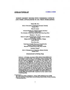
This section details the experiments that were conducted to compare semiparametric spectral approaches and fully parametric approaches to clustering of time-series data. k-Means and EM versions of a mixture of HMMs approach were used to represent the parametric setting. The two spectral clustering algorithms investigated were Yin and Yang’s algorithm[10], which computes a likelihoodbased kernel between pairs of sequences, and the SC-PPK algorithm which computes a kernel over the HMM model parameters. Note that there are parameters which can be adjusted for both of the spectral clustering methods: the σ fall-off ratio for the Yin-Yang kernel and the mixing proportion T for the SC-PPK method. In the following experiments, the default settings were used for both methods, i.e. σ = 1 and T = 10. Stability results for these kernels are shown in Fig 1.

170

5.1

T. Jebara, Y. Song, and K. Thadani

Datasets

The evaluations were run over a variety of real-world and synthesized datasets which are described below. MOCAP: The Motion Capture dataset (available from Carnegie Mellon University1 ) consists of time-series data representing human locomotion and actions. The sequences consist of 123-dimensional vectors representing 41 body markers tracked spatially through time for various physical activities. For these experiments, simple activities that were likely to be hard to cluster were considere; tests compared either similar activities or the same activity for different subjects. Table 2 contains the results of the evaluation over these real-world datasets. Rotated MOCAP: A synthesized dataset was generated by rotating two MOCAP sequences 5◦ at a time through 360 degrees. The seed sequences used were a walking sequence from walk(#7) and a running sequence from run(#9). This dataset, which provides us with clusters of sequences that lie on a regular manifold, is used for comparing clustering in Table 3, comparing running times in Table 6 and embedding in Fig 2. An additional dataset swerving was generated by rotating the walking and running sequence left and right periodically to make their movements seem zig-zagged. Arabic handwriting: This dataset consists of 2-dimensional time-series sequences which represent written word-parts of Arabic characters extracted from the dataset used in [11]. Table 4 shows the results of clustering pairs of similar word-parts (identified by their Unicode characters) and Fig 3(a) shows an MDS embedding of three symbols. Australian sign language: This dataset (from the University of CaliforniaIrvine2 ) consists of multiple sign-language gestures, each represented by 27 instances of 22-dimensional time-series sequences. Semantically-related expressions such as write and draw or antonyms such as give and take were assumed to have similar real-world symbols and formed the basis of all experiments with this dataset. Table 5 shows the average accuracy over the clustering of 18 such pairs of sequences while varying the number of HMM states used and Fig 3(b) shows an embedding of three gestures. 5.2

Results

The tables in this section show the results of experiments over these various datasets. Experiments were restricted to pairwise clustering over datasets of similar size. The standard accuracy metric is used for comparison of results. The results reported were averaged over multiple folds - five folds for the spectral clustering algorithms and ten folds for the fully parametric techniques since these algorithms converge to local maxima and have highly variable performance). In general, the kernel-based methods outperformed the parametric methods and the PPK performed favorably compared to Yin and Yang’s kernel. 1 2

http://mocap.cs.cmu.edu/ http://www.cse.unsw.edu.au/waleed/tml/data ˜

Spectral Clustering and Embedding with Hidden Markov Models

171

Table 2. Clustering accuracy with 2-state HMMs on MOCAP data. The numbers in the parentheses identify the index of the subject performing that particular specified action. Dataset k-Means EM Yin-Yang SC-PPK simple walk vs run set 100% 100% 100% 100% run(#9) vs run/jog(#35) 57% 52% 76% 100% walk(#7) vs walk(#8) 59% 60% 68% 68% walk(#7) vs run/jog(#35) 71% 69% 71% 95% jump(#13) vs jump forward(#13) 50% 50% 75% 87% jump(#13,#16) vs jump forward(#13,#16) 50% 50% 60% 66%

Table 3. Clustering accuracy with 2-state HMMs on synthesized MOCAP dataset. A single pair of walking and running time-series samples were used, subsequent samples were generated by rotating the seed pair 5◦ at a time to generate 72 unique pairs. rotation limit step size k-Means 30◦ 5◦ 100% 5◦ 54% 60◦ 5◦ 50% 90◦ 5◦ 51% 180◦ 5◦ 50% 360◦ 10◦ 50% 360◦ 15◦ 50% 360◦ 30◦ 54% 360◦ Swerving – 50%

EM Yin-Yang SC-PPK 100% 92% 100% 71% 63% 100% 50% 75% 100% 51% 71% 100% 50% 60% 100% 50% 50% 100% 50% 50% 100% 50% 50% 100% 50% 85% 100%

Table 4. Clustering accuracy with 2-state HMMs on Arabic handwriting dataset Dataset k-Means EM YY SC-PPK U0641 vs U0643 68% 64% 86% 97% 70% 66% 86% 100% U0645 vs U0647 U062D vs U062F 78% 80% 93% 95% 66% 65% 86% 93% U0621 vs U062D 71% 70% 94% 100% U0628 vs U0631 74% 76% 95% 100% U0635 vs U0644 71% 66% 96% 98% U0621 vs U0647

Improvements in accuracy well as better runtime performance were seen in both quantitative clustering accuracy and qualitative embedding performance. In addition, experiments were conducted to investigate the stability of the SC-PPK method over the T parameter. Fig 1 shows stability comparisons for both spectral clustering kernels over the respective parameters. The accuracies were averaged over five-fold testing. It was noted that a useful setting for T usually lay within the interval of 5 to 25. In practice, cross validation would be useful for recovering the optimal setting.

172

T. Jebara, Y. Song, and K. Thadani

Table 5. Clustering accuracy on Australian sign language dataset; 18 semantically related pairs of signs compared. Top: 5 representative pairs are shown for a range of SC-PPK clustering accuracies. Bottom: averages for the 18 pairs over different number of states. Sample pairs (2-state) ’hot’ vs ’cold’ ’eat’ vs ’drink’ ’happy’ vs ’sad’ ’spend’ vs ’cost’ ’yes’ vs ’no’ # of hidden states 2 3 4

k-Means 64% 52% 73% 58% 51% k-Means 64.5% 64.4% 65.4%

EM Yin-Yang SC-PPK 98% 96% 100% 50% 52% 93% 54% 50% 87% 53% 52% 80% 51% 52% 59% EM Yin-Yang SC-PPK 72.1% 69.3% 76.1% 73.3% 75.5% 75.5% 74.9% 74.7% 74.3%

Table 6. Average runtimes in seconds on a 3-Ghz machine with emissions xt ∈ R123×1 , includes HMM training time # of time-series samples k-Means EM Yin-Yang SC-PPK 5 20.6s 23.5s 4.1s 3.6s 47.1s 59.7s 11.1s 6.1s 10 68.29s 185.0s 49.9s 15.4s 25 111.6s 212.9s 171.8s 30.1s 50 178.3s 455.6s 382.8s 48.6s 75 295.9s 723.1s 650.2s 64.5s 100

5.3

Runtime Advantages

Unlike EM-HMM, which needs to calculate posteriors over N ×k HMM-sequence pairs and maximize over k HMMs at every iteration until convergence, SC-PPK requires a single HMM to be trained once for each sequence in the dataset. The SC-PPK method calculates the integration between two HMM parameters in closed form directly without needing to evaluate the likelihood of the individual time-series samples, resulting in a dramatic reduction of in total runtime. In practice, we noticed around two orders of magnitude improvement in clustering speed over EM, as shown in Table 6. These runtimes include HMM training times as well as clustering times.

6

Visualization of HMM Parameters

Visualization and manifold learning is another important component of unsupervised learning. Starting from a set of high dimensional data points X with xi ∈ RN , embedding and visualization methods recover a set of corresponding low dimensional datapoints Y (typically with typically yi ∈ R2 ) such that the

Spectral Clustering and Embedding with Hidden Markov Models Accuracy over σ − 5 fold testing 1

0.9

0.9

0.8

0.8

0.7

0.7

0.6

0.6 Accuracy

Accuracy

Accuracy over T − 5 fold testing 1

0.5

0.5

0.4

0.4

0.3

0.3

0.2

0.2 mocap: run9 vs walk7 arabic: u641 vs 643 Auslang: read vs write

0.1

0

173

0 5

10

15 T

(a)

20

mocap: run9 vs walk7 arabic: u641 vs 643 Auslang: read vs write

0.1

25

1

1.5

2

2.5

3 σ

3.5

4

4.5

5

(b)

Fig. 1. Kernel stability over their respective parameters (a) SC-PPK - T (b) YY kernel - σ. Accuracies averaged over five runs.

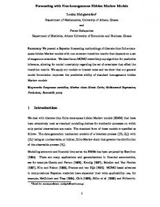
distance between yi and yj is similar to the distance between xi and xj for all i, j = 1...N . These techniques permit visualization of high dimensional datasets and can help confirm clustering patterns. Classic visualization and embedding techniques include multi-dimensional scaling (MDS) [12] as well as recent contenders such as semi-definite embedding (SDE) [13]. To further analyze the usefulness of the PPK at capturing an accurate representation of the kernel affinity between two sequences, embedding using MDS was applied to the datasets. This corresponds to training an HMM over each of the time-series sequences and recovering the RN ×N Gram matrix where Am,n = K(θm , θn ) – identical to steps 1 and 2 of the SC-PPK algorithm. From the Gram matrix, the dissimilarity matrix D ∈ RN ×N is given by Di,j = 1/Ai,j . This matrix is then used as the input for the standard MDS algorithm as in [12]. MDS is chosen because of its simplicity although more sophisticated methods such as SDE are equally viable. Fig 2 shows the embedding for the rotated data using a rotation step size of 10◦ under the Yin and Yang kernel (a) and the PPK (b). From the figure, we can see that the Yin and Yang kernel captures some of the periodic structure of the dataset in the embedding but it is only locally useful and does not adequately capture the expected global circular structure in the rotation. Conversely, the result from the PPK method is much clearer. The PPK integrates over the sample space providing a less brittle description of each time series. Thus the kernel affinity captures an accurate representation of the the distance between HMM parameters with respect to all of the data samples, forming a perfectly circular global embedding of the 360◦ rotated MOCAP dataset. Fig 3(a) shows PPK-based embeddings for three classes from the Arabic handwriting dataset. The method recovered an accurated embedding as the three classes are separated from one-another. Similarly, Fig 3(b) shows the embeddings for three classes from the Australian sign language dataset.

174

T. Jebara, Y. Song, and K. Thadani

15

x 10

2

0.5 0.4

1

0.3 0.2

0

0.1 0

−1

−0.1 −2

−0.2 −0.3

−3

−0.4

walking running

Walking Running −4

0

10

20

30

40

50

60

70

−0.5 −0.5

80

0

(a)

0.5

(b)

Fig. 2. MDS embedding of HMM parameters using the synthesized 360◦ rotated MOCAP dataset with (a) the Yin-Yang kernel and (b) the probability product kernel 0.4

0.3

0.3

0.2

0.2

0.1

0.1

0

0

−0.1

−0.1

−0.2

−0.2

−0.3 u62d u647 u621

−0.3 −0.4 −0.3

−0.2

−0.1

0

0.1

(a)

0.2

0.3

0.4

"Alive" "Building" "Computer"

−0.4

0.5

−0.5 −0.8

−0.6

−0.4

−0.2

0

0.2

0.4

0.6

(b)

Fig. 3. MDS embedding of HMM parameters (a) Arabic handwriting dataset and (b) Australian sign Language dataset

7

Conclusions

This paper presented a semi-parametric approach for clustering time-series data that exploits some parametric knowledge about the data including its Markov properties and the presence of latent states, and at the same time utilizes nonparametric principles and remains agnostic about the shape of the clusters a multitude of time series can form. This works surprisingly well for time-series data in experiments on real-world data. By avoiding parametric assumptions about the underlying distributions or the variations across the time series, improved clustering accuracy is possible. The method combines both a non-parametric spectral clustering approach using the probability product kernel with a fully parametric maximum likelihood estimation approach for each singleton time series. We showed that spectral

Spectral Clustering and Embedding with Hidden Markov Models

175

clustering with a probability product kernel method provides improvements in clustering accuracy over fully parametric mixture modeling as well as spectral clustering with non-probabilistic and non-parametric affinity measures. Furthermore, embedding and visualization of time series data is also improved. Finally, the proposed method has computational efficiency benefits over prior approaches. For future work, we are investigating spectral clustering with the probability product kernel for other generalized graphical models and parametric distributions. In addition, we are investigating a general formalism and generalized cost functions for semi-parametric estimation that unify both parametric and non-parametric criteria and leverage the complementary advantages of both approaches.

References 1. Dey, D.: Practical Nonparametric & Semiparametric Bayesian Statistics, vol. 133. Springer, Heidelberg (1998) 2. Hoti, F., Holstrom, L.: A semiparametric density estimation approach to pattern classification. Pattern Recognition (2004) 3. Tim Oates, L.F., Cohen, P.R.: Clustering time series with hidden Markov models and dynamic time warping. In: IJCAI-99 Workshop on Neural, Symbolic and Reinforcement Learning Methods for Sequence Learning (1998) 4. Smyth, P.: Clustering sequences with hidden Markov models. In: Advances in Neural Information Processing Systems, pp. 648–654 (1997) 5. Alon, J., Sclaroff, S., Kollios, G., Pavlovic, V.: Discovering clusters in motion timeseries data. IEEE Computer Vision and Pattern Recognition (2003) 6. Shental, N., Zomet, A., Hertz, T., Weiss, Y.: Pairwise clustering and graphical models. In: Advances in Neural Information Processing Systems (2003) 7. Ng, A., Jordan, M., Weiss, Y.: On Spectral Clustering: Analysis and an algorithm. In: Advances in Neural Information Processing Systems (2001) 8. Shi, J., Malik, J.: Normalized cuts and image segmentation. IEEE Transactions on Pattern Analysis and Machine Intelligence 22, 888–905 (2000) 9. Jebara, T., Kondor, R., Howard, A.: Probability product kernels. Journal of Machine Learning Research 5, 819–844 (2004) 10. Yin, J., Yang, Q.: Integrating hidden Markov models and spectral analysis for sensory timeseries clustering. In: Proceedings of the Fifth IEEE International Conference on Data Mining (ICDM’05), IEEE Computer Society Press, Los Alamitos (2005) 11. Biadsy, F., El-Sana, J., Habash, N.: Online arabic handwriting recognition using hidden Markov models. In: The 10th International Workshop on Frontiers of Handwriting Recognition (2006) 12. Kruskal, J.B., Wish, M.: Multidimensional Scaling. In: Quantitative Application in the Social Sciences, Sage University Paper (1978) 13. Weinberger, K.Q., Saul, L.K.: Unsupervised learning of image manifolds by semidefinite programming. International Journal of Computer Vision 70(1), 77– 90 (2006)