Spectral Clustering Approach - IIOA!

Detecting Energy Clusters from the Automobile Supply Chain: Spectral Clustering Approach

SHIGEMI KAGAWA†, YASUSHI KONDO‡, KEISUKE NANSAI*, & SANGWON SUH§

†

Faculty of Economics, Kyushu University, Fukuoka, Japan

‡

Faculty of Political Science and Economics, Waseda University, Tokyo, Japan, and

Industrial Ecology Programme, Norwegian University of Science and Technology, Trondheim, Norway *

Research Center for Material Cycles and Waste Management, National Institute for

Environmental Studies of Japan, Tsukuba, Japan §

Department of Bioproducts and Biosystems Engineering, University of Minnesota,

Minnesota, USA

Address for correspondence: Shigemi Kagawa, Faculty of Economics, Kyushu University, 6-19-1 Hakozaki, Higashi-ku, Fukuoka, 812-8581, Japan, Phone and Fax: +81-92-642-2489, [email protected].

1

ABSTRACT This paper proposes a new method that identifies energy-intensive industrial clusters from product supply chains quantitatively by combining structural path analysis and spectral clustering analysis. The analysis of automobiles has engendered the discovery of numerous clusters joining the upstream and downstream sectors together such as a cluster that consists primarily of three sectors––electrical equipment for internal combustion engines (#244), internal combustion engines for motor vehicles and parts (#250), and motor vehicle parts and accessories (#251)––which reveals a composition of sectors that differs considerably from the current Japan Standard Industrial Classification. This paper also proposes the “within-cluster effect” as a new indicator of energy intensity inside the industrial clusters identified from the automobile supply chain and presents quantitative analyses of the importance of industrial clusters in terms of the environment.

Key words: Energy clusters, automobile supply chain, structural path analysis, spectral clustering analysis

2

1. Introduction

According to the database of sectoral carbon dioxide emissions provided by the National Institute for Environmental Studies of Japan (NIES)1, the total of carbon dioxide emissions emitted directly through production activities of firms, increased by 27 million tons-C during the period from 1990 to 2000. Consequently, the total emissions increased by 9.5% during those ten years. In these circumstances, energy-intensive sectors such as electricity, iron and steel, cement, and transportation have received attention as target sectors for the simple reason that total emissions at a domestic level can be reduced efficiently by promoting energy-saving technologies of these sectors.

In implementing sector-wise environmental and energy policies, it is crucial not only to clarify the concept and definition of sectors (e.g., firms, industries, or commodities) but also to decide their priority levels based on reliable environmental inventories such as CO2 intensities and energy intensities. In these respects, the environmental input–output analyses are useful not only for estimating commodity-wise and industry-wise environmental inventories, but also for identifying the environmentally important key sectors using economic statistics that are calculable from the backward and forward inter-industry linkage effects obtained from column and row sums of the direct and indirect intermediate input coefficient matrix (see Rasmussen, 1956; Hirschman, 1958; Bharadwaj, 1966; Hazari, 1970; Lenzen, 2003).

A recent interesting discussion is that not only net multipliers developed by Oosterhaven and Stelder (2002) can be used to avoid double counting of the total impact of an industry 1

See http://www-cger.nies.go.jp/publication/D031/eng/table/embodied/f_embodied.htm, visited at September 18, 2009.

3

which results from multiplying a certain input–output multiplier by the industrial output but also, as Dietzenbacher (2005) discovered, that net multipliers yield a relevant key sector indicator obtained by dividing the total backward linkage effect of industry j by the total forward linkage effect of industry j (see eq. (3) of Dietzenbacher (2005)). For a recent empirical contribution, Lenzen (2003) identified environmentally important paths, linkages, and key sectors in the Australian economy using weighted and unweighted coefficients of variation derived from backward and forward inter-industry linkage effects. In addition, an alternative key sector approach is to use both in-degrees and out-degrees obtained from column and row sums of the adjacency matrix represented as a {0, 1}-matrix, where 1 denotes an influential inter-industry transaction larger than (or greater than) a certain threshold value, otherwise 0 (see e.g., Ghosh and Roy, 1998; Kagawa et al., 2009 for graph-theoretic analyzes and part II of Lahr and Dietzenbacher (2001) for the theoretical remarks and its applications of the qualitative input–output analysis using the adjacency matrix).

Although sector-wise analyses such as key sector analysis described above indicate key sectors that pollute environment through energy consumption induced by production of energy and materials needed for the production in the sector in question, they are naturally limited to policy implications within a sector rather than between sectors. We also think that it is important to give some incentive to cooperate between different sectors and to attain the same goal of reducing the total environmental burden associated with supply chains from upstream sectors to downstream sectors. Especially, to save energy and reduce environmental burdens efficiently, it is very effective to identify energy-intensive industrial clusters objectively from the supply chains of goods and services in question and provide that information to the public. Thereby, not only are the respective levels of social responsibility of a particular industrial cluster and industries within the cluster in question revealed and ranked, the importance of reducing environmental burdens through cooperation among 4

different sectors within the relevant cluster can be emphasized.

In the field of regional studies, many contributions have been put forth in attempts to identify regional and industrial clusters and complexities (see Streit, 1969; Roepke et al., 1974; Czamanski and Ablas, 1979; Feser and Bergman, 2000; Oosterhaven et al., 2001, Feser et al., 2005; Kelton et al., 2008). Their studies normally calculated the relevant four correlation coefficients representing the following similarities between two industries: (1) Industries u and v have similar input purchasing patterns, (2) Industries u and v have similar output selling patterns, (3) The buying pattern of industry u is similar to the selling pattern of industry v, (4) The buying pattern of industry v is similar to the selling pattern of industry u and identified the industrial clusters by application of the similarity matrices to principal component factor analysis (e.g., varimax method and promax method). The bottom-up type cluster methods based on economic distances (e.g. technological similarity) are called polythetic methods. In a relevant remark, Oosterhaven (2001, p.811) reported that:

“The use of the phrase ‘relatively closely [relative similarity]’ indicates that the drawing of the border of any cluster,…, will always involve a certain arbitrariness.”

It is noteworthy that determining the number of clusters is regarded as a most difficult problem in the field of discrete mathematics (see, e.g. von Luxburg, 2007).

As described herein, we demonstrate that a popular heuristic approach––the Spectral Clustering Approach––is extremely useful for addressing the industrial cluster problem (see section 1.1 of Spielman and Teng (2007) for the short history and Chung (1997) for the related mathematical properties). In fact, although many applied studies have been made in the field of parallel computing (e.g., Hendrickson and Leland, 1995) and image segmentation (Shi and 5

Malik, 2000), apparently very few studies have been undertaken in an attempt to detect the industrial clusters using the spectral clustering theory in the field of applied economics. In a related study, Aroche-Reyes (2003) definitively introduced a “network cut criterion” to draw the border of any cluster and identified a tree of the fundamental production structure for Mexico using input–output tables. However, Aroche-Reyes (2003) did not use the spectral graph approach but instead used Prim’s algorithm to detect the spanning tree of the Mexico economy. An important feature of the spectral clustering theory is that the border of any cluster can be drawn based on a criterion (cut value, normalized cut value, etc.) (see von Luxburg, 2007; von Luxburg et al., 2008). Consequently, the spectral clustering theory is called a monothetic method. The well-known triangulation methods of input–output matrix also belong to a family of the monothetic methods because they depend largely on a criterion of maximizing the degree of linearity and check the relevance of the matrix triangulation (see Simpson and Tsukui, 1965; Fukui, 1986; Howe, 1991; Dietzenbacher, 1996). We understand that both spectral clustering (graph partitioning) and block triangulation from the input–output theory belong to a family.

This study employs the latter, the spectral clustering method, and attempts to identify the energy-intensive clusters by minimizing the normalized cut value consisting of the energy consumption of the sectors within the cluster in question as the denominator and the energy consumption induced by the economic linkage among the clusters as the numerator (i.e. energy cut value). More specifically, applying the 2000 environmental input–output database to the spectral clustering method, we attempted to detect the environmentally important clusters from the supply chain of the automobile sector as a case study, which plays a crucial role in the Japanese economy. Subsequently, we argued that peculiar features of the energy intensive clusters of the Japanese auto sector and policy present implications of saving energy effectively through cooperation among different sectors within the clusters. 6

This paper is organized as follows: Section 2 reconciles structural path analysis with spectral clustering analysis, Section 3 describes the data sources and Section 4 presents the empirical results obtained by application of the 2000 environmental input–output table of Japan to the spectral clustering analysis and discusses the relevance of the energy-intensive clusters from the automobile supply chain in 2000 and presents quantitative analyses of the importance of the industrial clusters of auto industry in terms of the environment by using the proposed new indicator “within-cluster effect” showing energy intensity inside the industrial clusters. Section 5 explains about the nested structure of detected energy-intensive clusters and Section 6 explains the related policy implications. Finally, Section 7 concludes the paper.

2. Reconciling structural path analysis with spectral clustering

A starting point is that we define the input coefficient matrix as A = (aij ) (i, j = 1,… n) representing a million yen’s worth of intermediate input of commodity i per million yen of

output of commodity j, where n refers to the number of commodities (see e.g., chapter 2 of Miller and Blair, 2009). If the consumption (unit: gigajoule, GJ in SI) of energy resource k directly required for a unit of output of commodity j is defined as the direct energy intensity matrix, E = (ekj ) , then the total direct energy consumption for a unit of output of commodity j ~ is obtainable as the direct energy intensity vector E = sE , where s is the summation row

vector in which all the elements are unity. Furthermore, we define a diagonal matrix in which

~ ~ each element of E = (~ e j ) is diagonalized as diag(E) . As sectoral energy consumption C = (Ci ) that is directly and indirectly attributable to automobile production is provided by the following equation. 7

~ ~ −1 C = diag(E) X auto = diag(E)(I − A ) Fauto ~ ~ ~ ~ = diag(E)Fauto + diag(E) AFauto + diag(E) A 2Fauto + diag(E) A 3Fauto +

−1

Here X auto = (I − A ) Fauto , I is the identity matrix with appropriate order and Fauto is the domestic final demand vector in which only the element associated with only automobile sector has a figure; all other elements are zero.2 The energy intensity for the production of the intermediate goods and services flowing from sector i to sector j can be estimated as the (i,

~ j)-element of the matrix diag(E) A . On the other hand, because the productions of the intermediate goods and services necessary to produce the domestic final demand (in a million yen’s worth) of, for instance, automobiles are calculable as AFauto , the energy consumption (unit: GJ) necessary to produce commodity i purchased for the production of commodity j directly required for producing the domestic final demand of automobiles can be estimated as ~ the (i, j)-element of diag(E) Adiag(AFauto ) , where diag( AFauto ) represents the diagonal

matrix whose diagonal elements are products of intermediate goods and services induced directly by the final demand for automobile. Noting that this economy produces automobiles and intermediate goods and services that are directly demanded for producing the automobiles and that the economy consumes energy to produce them at downstream stages, the energy consumption (unit: GJ) necessary to produce commodity i purchased for the production of commodity j directly and indirectly for producing the domestic final demand of automobiles,

Q = (Qij ) (i, j = 1,

2

, n) , can be finally estimated as

The matrix (I − A) = B = (bij ) is well known as the Leontief inverse matrix showing the direct and indirect input of −1

commodity i required for the final demand of commodity j (see e.g., chapter 2 of Miller and Blair, 2009).

8

~ ~ Q = diag(E)diag(Fauto ) + diag(E) Adiag(Fauto ) ~ ~ + diag(E) Adiag(AFauto ) + diag(E) Adiag(A 2Fauto ) +

,

(1)

where the first term on the right-hand side of eq. (1) represents the matrix in which the diagonal element associated with only automobile sector records the energy consumption required at automobile plants and the other diagonal and off-diagonal elements are zero. The second term represents the matrix in which the ith row element of the column associated with automobile sector records the energy consumption necessary to produce an intermediate good or service i required for producing automobiles and the other matrix elements are zero.3 Summing up higher order terms results in an increase in the non-zero elements. In other words, the inclusion of higher order terms increases the number of sectors participating in inter-industrial networks.

The matrix Q = Qij (i, j = 1,

, n) in eq. (1) can be regarded as a weighted directed

graph showing the flow from an upstream sector i to a downstream sector j. A graph

G = (V , A) can be reasonably derived from Q such that the set of vertices is V = {1,…, n} , the set of arcs (or directed edges) is A = {(i, j ) | Qij > 0} , and the weight assigned to edge (i, j ) is Qij . The weight of the flow is the energy consumption necessary to produce commodity i upstream purchased for the production of commodity j downstream. It is important that more direct energy consumption required for automobile production be considered and that a major upstream sector i with high-induced energy consumption Ci associated with automobile production participates in the inter-industrial network. This makes it easier to discuss the features of the inter-industrial network and detected industrial clusters 3

This study uses the same name for both the industrial sector and commodity sector for the industries producing the commodity concerned as the primary product. For instance, the automobile industry produces automobiles as its primary product. It is therefore called the automobile industry.

9

from the point of view of technological linkages. This study therefore defines the adjacency matrix by summing up the lower order terms shown in the right-hand side of equation (1) such that major high-ranking sectors with high-induced energy consumption participate in inter-industrial networks.

This study uses the sums of the amounts of energy consumption from sector i to sector j and from sector j to sector i as indicators of the strength of the relation through inter-sectoral energy consumption. For particularly addressing the energy consumption associated with the inter-sectoral transactions, a symmetric matrix Q* = (Qij* ) (i, j = 1,…, n) with the diagonal element (the energy consumption of the sector itself) set to zero is defined as shown below to examine the non-diagonal elements specifically.

Qij* = Qij + Q ji

(i ≠ j ),

Qij* = 0 (i = j ).

In what follows, we presents the network analysis based on a weighted undirected graph derived from the matrix Q* . Some notations are introduced before going into details of the analysis. Let QCD denote the matrix is in which the elements Qij (i ∈ C , j ∈ D) of Q for subsets C , D of V are arranged. For instance, when C = {1,3} and D = {2,3, 6} , then

⎡Q QCD = ⎢ 12 ⎢Q32 ⎣

Q13 Q33

Q16 ⎤ ⎥, Q36 ⎥⎦

and also Q = QVV . Although the sets of row and column indices should be ordered sets rather than proper sets to be more precise, the difference between these two is not necessary and is 10

therefore not examined. In addition, the sum of all elements of the matrix QCD is expressed as

QCD = ∑∑ Qij . i∈C j ∈ D

The same notations for subscripts and the sum of elements are used for Q* . In some cases,

QCD is written as Q(C , D) instead to avoid nested subscripts.

Here we seek to detect energy-intensive industrial sub-networks from the automobile supply chain by partitioning the set of vertices of graph G = (V , E ) into two disjoint sets of sectors, C and D, where the graph is derived from the symmetric matrix Q* defined above such that the set of vertices is V = {1,2,

, n} and the set of edges is

E = {(i, j ) | Qij* > 0, i < j} . If two sectors in question, u and v respectively belong to sets C

and D, then the cut value in the Graph Theory is definable as follows (see e.g., Shi and Malik, 2000)

Cut (C , D ) = Q*CD =

∑

Quv* .

(2)

u ∈C ,v∈ D

Cut (C , D) = Cut ( D, C ) because Q* is symmetric. The cut value is understood to be the

energy intensiveness of the transactions between two industry groups C and D. To detect the most energy-intensive industrial clusters from the whole supply chain, it is necessary to find the two sets to minimize the energy intensiveness between two industrial groups (i.e. cut value). Consequently, to minimize the cut value is environmentally meaningful. However, as Wu and Leahy (1993) and Shi and Malik (2000) pointed out, one shortcoming of the cut criterion in eq. (2) is that the cut criteria force the cutting of small sets of isolated sectors. 11

Therefore, following Shi and Malik (2000), the normalized cut value is used in this study to avoid that undesirable solution. The normalized cut value can be formulated as

Q*CD Q*DC Cut (C , D) Cut ( D, C ) Ncut (C , D ) = + = * + * , vol (C ) vol ( D ) QCV Q DV

where vol(C ) = Q*CV

(3)

and vol( D ) are similarly defined. If the weighted degree of each

sector u is defined as d u = ∑ Quv* , then eq. (3) can also be reformulated as v∈V

Ncut (C , D ) =

Cut (C , D ) Cut ( D, C ) + . ∑ du ∑ dv u∈C

(4)

v∈ D

In eq. (4), the clustering problem is to find the two sets C and D such that not only the cut value (i.e. the numerator) is minimized but also the sizes of both clusters (the denominator) are maximized simultaneously. Our optimization problem is therefore formulated as follows.

minimize Ncut (C , D) subject to C ∪ D = V , C ∩ D = ∅

(5)

Here it is well known that this problem is an NP-complete problem. In an influential paper by Shi and Malik (2000), they further transformed eq. (5) into the following equivalent optimization problem.

12

y T ( D − Q* ) y

minimize

y T Dy

subject to y T Di = 0

(6)

yi ∈ {1, −b} (i = 1, …, n)

Here, the superscript T denotes the transpose of the vector, y = ( yi ) (i = 1,

, n) is the

transformed indicator vector, D is the diagonal matrix whose diagonal elements are weighted degrees du , i is the vector of unities, and

b = ∑ di i∈Y

∑d

i

with Y = {i ∈ V | yi = 1}

i∈V -Y

(see p. 890 of Shi and Malik (2000)). In fact, D − Q* is often called the Laplacian matrix and normally denoted by L in the Graph Theory. It is noteworthy that the optimization problem in eq. (6) is still an NP-complete problem.

The objective function of the optimization problem (6) is the form of the Rayleigh quotient for the generalized eigenvalue problem (D − Q* )y = λDy where λ is the eigenvalue and y is the corresponding eigenvector (see e.g. Chapter 7 of Bellman (1997) for the Rayleigh quotient). Once the indicator vector y in eq. (6) is relaxed to take on ‘real values’, the optimization problem immediately engenders the following problem to find the second smallest eigenvalue and the corresponding eigenvector.

minimize

y T ( D − Q* ) y y T Dy

(GEP( Q* )) subject to y T Di = 0 yi ∈ R (i = 1, …, n)

13

(7)

Therein, (GEP( Q* )) refers to the generalized eigenvalue problem using the adjacency matrix Q* . That the smallest eigenvalue of the generalized eigenvalue problem is 0 and the

eigenvector corresponding to the smallest eigenvalue is the unity vector i is well known: from the definitions of D and Q* , we have (D − Q* )i = λDi = 0 where 0 is the null vector.

Defining w = D1/ 2 y , eq. (7) can be further transformed as

minimize

w T D−1/ 2 (D − Q* ) D−1/ 2 w

wTw subject to w T D1/ 2 i = 0

.

(8)

wi ∈ R (i = 1, …, n)

The smallest eigenvalue of the normalized Laplacian matrix D−1/ 2 (D − Q* ) D−1/ 2 is 0 and the corresponding eigenvector is D1/ 2 i . Therefore, an optimal solution to the problem in (8) with the orthogonal condition w T D1/ 2 i = 0 invariably provides the eigenvector corresponding to the second smallest eigenvalue. The second smallest eigenvalue of the normalized Laplacian matrix is called the Fiedler eigenvalue (see Fiedler, 1973; Chung, 1997); the eigenvector corresponding to the Fiedler eigenvalue is called the Fiedler eigenvector.

Using the matrix elements, eq. (8) can also be rewritten as (see, e.g., pp. 12–13 of Chung (1997))

14

⎛ w j ⎞⎟⎟ wi *⎜ ⎜ − Q ⎟ ∑∑ ij ⎜ ⎜⎜⎝ di d j ⎠⎟⎟ i =1 j =1

2

n

minimize

n

n

∑w

2 i

i =1

n

∑w

subject to

di = 0

i

,

(9)

i =1

wi ∈ R (i = 1, …, n)

or equivalently,

n

n

∑∑ Q ( y − y )

2

* ij

minimize

i

j

i =1 j =1

n

∑d y i

2 i

i =1

n

subject to

∑d y i

i

=0

.

(10)

i =1

yi ∈ R (i = 1, …, n)

An important feature of eqs. (9) and (10) is that, as Shi and Malik (2000) explained in their paper, the optimization problem forces the elements of the vector y = D−1/ 2 w to take similar values for sectors i and j that induce a large amount of energy by the bilateral transaction and form the energy-intensive transaction. In summary, if industrial sectors are found which have similar indicator vector values ( −b or 1 in the original optimization problem), then the industries in question will form an energy-intensive industrial cluster.

Turning to a precise description of our method, set r = 20 as the prescribed value for the maximum allowable number of sectors in a cluster to control the following recursive two-way cut algorithm. We assume that any sector, say u , is not isolated from the other sectors in V , i.e. d u > 0 for every u ∈ V . That is, any sector is assumed to purchase outputs of other sectors or to be purchased by other sectors. It is notable that the graph to be 15

analyzed is not necessarily connected. We seek to partition V into clusters that have the same features because we believe that a set with isolated sectors does not deserve to be called a cluster. In the recursive two-way cut algorithm, therefore, we do not partition a graph, or sub-network, any cut of which invariably induces sub-networks with isolated sectors even if the number of sectors in it is larger than the maximum allowable number, r . Then, the computational algorithm is presented as follows.

16

Step 0. Set k := 0 , j := 0 and Ω := {V } . Step 1. If Ω ≠ ∅ , then set N := k and N = j and terminate the algorithm. Otherwise, set

j := j + 1 , choose a set of sectors V j ∈ Ω , and set Ω := Ω− {V j } and Q*jj := Q* (V j , V j ) .

Step 2. If the number of sectors in V j is smaller than or equal to the prescribed value r , i.e. if V j ≤ r , or any cut of V j invariably induces sub-networks with isolated sectors, then set k := k + 1 and S k := V j , and go to Step 1.

Step 3. Solve the generalized eigenvalue problem GEP( Q*jj ) in (7) and obtain the eigenvector

y that corresponds to the second smallest eigenvalue. Step 4. Set C := {u yu ≥ 0}, D := {v yv < 0} and Ω := Ω ∪ {C , D}.

Step 5. Go to Step 1.

The computation was done using software (Matlab; The MathWorks Inc.). When the algorithm terminates, we are left with N sub-networks and their sets of vertices and associated weight matrices are V1 ,…, VN and Q11 ,…, Q NN , respectively. In addition, N of the N sub-networks are clusters and their sets of vertices are S1 , …, S N . Actually, S1 ,…, S N are exhaustive and mutually exclusive subsets of the set of all the industrial sectors V , i.e.

S1 ∪

∪ S N = V and Si ∩ S k = ∅ (i, k = 1, …, N ; i ≠ k ) . Let p(k ) denote the index of a

sub-network such that it is the k -th cluster is the p(k ) -th sub-network, i.e. V p ( k ) = Sk . It is noteworthy that a sub-network, say j , has its two “children”, h and i such that

V j = Vh ∪ Vi and Vh ∩ Vi = ∅ unless it is a cluster. 17

Therefore, we used the recursive two-way cut algorithm and detected the energy clusters of the Japanese automobile supply chain in 2000. Here let us recall that the matrix Q = (Qij )

(i, j = 1, , n) represents the energy consumption (unit: GJ) that is necessary to produce commodity i purchased for the production of commodity j required for the production of automobiles. Accordingly, this automobile supply chain totally consumes energy of Q . It is noteworthy that we obtain the relation Q* = 2 Q . The total amount of energy consumption, Q , can be decomposed as

Q = Q p (1) p (1) + Q p (1) p (2) + + Q p (2) p (1) + Q p (2) p (2) +

+ Q p (1) p ( N ) + Q p (2) p ( N )

+ + Q p ( N ) p (1) + Q p ( N ) p (2) +

where Qij = Q(Vi ,V j ) . Furthermore, Q p ( k ) p ( k )

(11)

+ Q p( N ) p( N )

represents the subtotal of energy induced by

the intermediate inputs between the sectors belonging to the k -th cluster. We designate

Q p(k ) p(k )

as a within-cluster effect of cluster k . Using the proposed index, we evaluated

the relevance of energy-intensive clusters of the automobile supply chain and the temporal changes in the within-cluster effects during the period of 2000.

18

3. Data Sources

As described in this paper, we specifically examined the 33 primary and secondary energy resources (Coking coal, Steam coal, lignite and anthracite, Coke, Blast furnace coke, Coke oven gas, BFG consumption, BFG generation, LDG consumption, LDG generation, Crude oil, Fuel oil A, Fuel oils B and C, Kerosene, Diesel oil, Gasoline, Jet fuel, Naphtha, Petroleum-derived hydrocarbon gas, Hydrocarbon oil, Petroleum coke, LPG, Natural gas, LNG, Mains gas, Black liquor, Waste wood, Waste tires, Recycled plastic of packages origin, Nuclear power generation, Hydroelectric and other power generations, Electric power for enterprise use, and On-site power generation). We compiled the energy inputs in calorific units (GJ) necessary for the respective sectoral production processes in monetary units (million yen), which data are obtainable from the Japanese Benchmark Input–Output Table in 2000 producer’s prices (393 sectors) (see Nansai et al., 2007, 2009 for more details and Table A1 of the appendix for the sector classification). The primary and secondary energy resources are categorized into 5 energy sectors (see Table A2 of the appendix for the energy sector classification).

From the energy input–output database, the total energy consumption of each sector is calculable by summing up the energy inputs of each sector. The direct total energy intensity of

e j , is obtainable by dividing the total energy consumption by the sectoral production. sector j, ~ It is noteworthy that summing up the energy inputs that belong to an energy category in question and dividing the calculated total energy consumption of the energy category by the sectoral production readily yields the direct total energy intensity of each energy category of sector j. Finally, we obtained the (393 × 393) diagonal matrix with total energy intensities and constructed the adjacency matrix of energy consumptions Q by substituting the energy

19

()

~ intensity matrix diag E , input coefficient matrix A from the benchmark input–output table, and the diagonalized matrix for the automobile domestic final demand (i.e., household consumption expenditure of automobile + fixed capital formation of automobile + increase in stock of automobile) diag(Fauto ) into the right-hand side of eq. (1).4

4. Case study of the Japanese automobile supply chain in 2000

The fundamental idea of the aforementioned sectoral approach is to reduce carbon dioxide emissions by extracting energy-intensive sectors from a supply chain from its upstream to downstream sectors and demanding that such sectors take further energy conservation measures. For example, this means that increased promotion of energy conservation in individual sectors would require further reduction of the power needed for the operation of the production lines of these auto-parts manufacturers. Parts assembly manufacturers, however, have already been making efforts to conserve energy through means such as the implementation of systems to monitor energy consumption in their production process to check their power consumption meticulously at each production line. The current situation, therefore, is that further energy conservation and carbon emission reduction through the efforts of individual parts assembly manufacturers is difficult to achieve.

Under such circumstances, heterogeneous (intersectoral) industry cooperation is expected to facilitate future energy-saving measures and carbon emission reduction. An important question to ask is which sectors need to cooperate mutually to reduce energy consumption and carbon dioxide emissions more effectively. More specifically, which 4

In Japan, the final demand of automobiles purchased by households is recorded in the household consumption expenditure, while the final demand of automobiles purchased by firms is recorded in the fixed capital formation.

20

material producers the assembly manufacturers must closely collaborate with is the question that must be answered to advance their effort to conserve energy. One way is to select the sectors subjectively based on knowledge from various experiences and then regard the group of these sectors as a cluster (group), and demand that they strengthen their operational ties for energy saving. This method, however, causes the arbitrary judgment of the analyzer and policy-maker to affect the final decision about the cluster significantly. Avoiding such arbitrary decision-making requires objective methods of some kind.

The new method proposed in Section 2 enables us to objectively detect the energy-intensive clusters from the automobile supply chain. From eq. (1), this study redefines the adjacency matrix, which is shown below as the total up to the quadratic terms so that the 30 high-ranking sectors with a large amount of induced energy consumption by sector will participate in the inter-industrial networks.

~ ~ ~ Q = diag(E)diag (Fauto ) + diag(E) Adiag(Fauto ) + diag(E) Adiag (AFauto )

It should be noted that the total of the induced energy consumptions ( Ci ) of these top 30 n

sectors comprises more than 90% of the sum total

∑C i =1

i

of induced energy consumption.

A cluster can be extracted objectively from a network using the spectral clustering approach formulated in the previous section. More specifically, first, the adjacency matrix Q* that expresses the weighted undirected graph is calculated using the adjacency matrix

Q = (Qij ) (i, j = 1,

, n) that expresses the weighted directed graph. Then, the solution to

the problem GEP( Q* ) given by eq. (7), i.e., the second eigenvector y of the generalized

(

)

eigenvalue problem D − Q* y = λDy , is obtained, and the network is divisible into two 21

highly energy-intensive sub-networks using the signs of the elements of y .

Sorting the elements of the calculated second eigenvector in ascending order yielded the following vectors.

#128 ⎡ −7.92 × 104 ⎤ ⎢ ⎥ # 78 ⎢ −6.97 × 104 ⎥ # 73 ⎢ −6.82 × 104 ⎥ ⎢ ⎥ #80 ⎢ −6.13 × 104 ⎥ ⎢ ⎥ ⎢ ⎥ # 263 ⎢ −3.52 × 108 ⎥ #130 ⎢ −2.91× 108 ⎥ ⎢ ⎥ #357 ⎢ −1.31× 108 ⎥ #378 ⎢⎢ −2.83 × 109 ⎥⎥ y* = #341 ⎢ 2.70 ×107 ⎥ ⎢ ⎥ #114 ⎢ 3.55 × 107 ⎥ # 274 ⎢ 4.63 ×107 ⎥ ⎢ ⎥ #96 ⎢ 5.60 ×107 ⎥ ⎢ ⎥ ⎢ ⎥ # 232 ⎢ 1.09 × 105 ⎥ #165 ⎢ 1.13 ×105 ⎥ ⎢ ⎥ #164 ⎢ 1.60 × 105 ⎥ ⎢ ⎥ #163 ⎢⎢⎣ 1.60 × 105 ⎥⎥⎦

sgn( yi* ) < 0

sgn( yi* ) > 0

where sector numbers corresponding to the elements are added as notations on the left border of the second eigenvectors. By particularly addressing the sign of the elements of this second eigenvector, the entire network is divisible into two sub-networks – one comprising the sectors belonging to the set of V2 = {#128 (synthetic fibers), #78 (yarn and fabric dyeing and finishing (processing on commission only)), #73 (fiber yarns), #80 (carpets and floor mats), … , and #378 (other amusement and recreation services)} and the other composed of the

sectors belonging to the set of V3 = {#341 (research institutes for natural sciences (private, 22

non-profit)), #114 (petrochemical aromatic products (except synthetic resin)), … , and #164 (crude steel (electric furnaces), #163 (crude steel (converters))}. If the number of sectors belonging to these sub-networks that have been identified is equal to or smaller than the maximum allowable number of sectors, which is set as r = 20 in this study, they are determined as a cluster. The number of sectors belonging to the sets V2 and V3 , however, exceeds this maximum allowable number of sectors. Therefore, each of the sub-networks formed by the sectors belonging to these sets is divided further into two. In concrete terms, the algorithm is Ω = {V2 , V3 } at this stage. Therefore, one of its elements, i.e. a sub-network that has been detected, is selected. We assume that V3 has been selected. The adjacency matrix

Q*33 = Q* (V3 ,V3 ) that corresponds to this sub-network is defined and the solution to the problem GEP( Q*33 ) given by eq. (7) is obtained. Sub-network V3 is further divided into two sets of industrial sectors, V4 and V5 , based on the sign of the elements of the solution. Subsequently, we determine whether the number of sectors in each of V4 and V5 is greater than the maximum allowable number of sectors. If it does not, the sectors are determined as a cluster and if it does, the sub-networks detected are divided into two again in the same way. These steps are repeated until the calculation is stopped when there is no sub-network which has not been divided into two yet and should be divided because the number of sectors is greater than the maximum allowable number of sectors and further division without producing isolated sectors is possible.

As a result of the analysis, 27 clusters were detected. Although all 27 clusters cannot be described in this article because of space limitations, the results related to the top ten clusters with high “within-cluster effect ( Q p ( k ) p ( k ) )” formulated in the previous section are reported in the following.

23

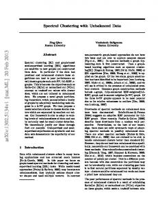
(1) Motor vehicle parts and accessories cluster Figure 1 presents the five clusters from the highest within-cluster effects. The clusters that have the highest within-cluster effect at approximately 20.7 PJ and is the most energy-intensive in the automobile supply chain is the cluster consisting primarily of three sectors including “electrical equipment for internal combustion engines (#244),” “internal combustion engines for motor vehicles and parts (#250),” and “motor vehicle parts and accessories (#251)" as indicated in Fig. 2. Calculation of the degrees of the sectors in this cluster revealed that the degree of “motor vehicle parts and accessories (#251)” was the highest; for this reason, this cluster is named the “motor vehicle parts and accessories cluster” for convenience. The other clusters that were detected were also named similarly. Figure 1 presents consumption by type of energy of the within-cluster effect of this cluster as 9.1 PJ for power consumption and 5.7 PJ for petroleum-based consumption, which comprise approximately 44% and 28%, respectively, of all consumption. These data suggest that the reduction of power consumption and petroleum-based energy in the cluster is the most important issue. Examination of the weight on the edges (i.e. the energy consumption induced by the inter-sectoral transactions) in the graph (the cluster) indicated in Fig. 2 reveals a particularly strong connection of the three major parts assembly manufacturers described earlier with three sectors made up of “cast and forged materials (iron) (#171),” “non-ferrous metal castings and forgings (#182),” and “bolts, nuts, rivets and springs (#188)” in the motor vehicle parts and accessories cluster. According to the information related to the Web site shown by Kinki Forging Cooperative Association (http://www.kintan.jp/forging.html), forged materials are used everywhere on automobiles, as connecting rods, crankshafts, rocker arms, various gears, constant-velocity joints, clutch hubs, and wheels. The development of forged materials therefore constitutes an important key to solving the conflict between the weight reduction of car bodies to improve the fuel-efficiency and hardening of car bodies to ensure collision safety (Osakada, 2009). These estimation results suggest that material development 24

is important not only to improve fuel efficiency and ensure collision safety on the part of end users through the industrial cooperation between auto-parts manufacturers and forged material manufacturers, but also to reduce energy consumption at the stage of manufacturing forged materials (ferrous and nonferrous) through the development of such materials. In particular, manufacturing of forged materials generally uses not only fuels such as fuel oil and kerosene as heating agents, but a large amount of electric power to operate hammers and forging machines for press (heavy equipment). In addition to the development of forged materials, the manufacturers of forged materials themselves are able to conserve energy of the entire automobile supply chain efficiently by making efforts to reduce the consumption of such energy. The power conservation in the use of forging machinery (heavy equipment) would naturally require cooperation between forged material manufacturers and heavy equipment manufacturers.

[Insert Figure 1 here]

[Insert Figure 2 here]

(2) Sheet glass and safety glass cluster Modern cars are lumps of iron and can also be considered lumps of glass. Because of this, it is easily imaginable that a cluster consisting largely of glass manufacturers will be detected. This analysis caused the detection of this cluster as having the second highest within-cluster effect (c.f. Fig. 1). The consumption by type of energy of the within-cluster effect in Fig. 1 reveals that, in particular, the crude oil-based energy and electric power comprise approximately 60% and 31%, respectively, of all consumption in this “sheet glass and safety glass cluster,” suggesting that the reduction of these types of energy is the priority 25

issue. Figure 3 portrays this cluster’s shape, which reveals that the inter-sectoral transactions, among others, from ”materials for ceramics (#29)” and “industrial soda chemicals (#108) to “sheet glass and safety glass (#149)” and to “passenger motor cars (#246),” are energy-intensive. Especially, glass manufacturing uses a large amount of fuel oil for melting raw materials such as silica sand and soda ash (Na2CO3), which increases crude oil-based energy consumption in the cluster. Glass manufacturing can be expected to reduce its carbon dioxide emissions by substituting natural gas for the fuel oil required in the melting process (Nippon Electric Glass Co., Ltd., 2009). Although tempered glass for automobiles (windshield, windows, etc.) is demanded to offer various features such as shock resistance, safety, insulation, blocking ultraviolet rays, and water repellence, design to reduce to the greatest extent possible the amount of energy-intensive glass used through measures such as weight reduction is needed. The technology for laminated glass (an intermediate membrane is inserted between two sheets of glass) has been developed in recent years, supporting the development of materials that can ensure both weight reduction and safety. It is important that auto-manufacturers adopt such materials with high environmental performance and also that they collaborate closely with glass manufacturers to design glass that meets the market needs.

[Insert Figure 3 here]

(3) Motor vehicle bodies cluster As portrayed in Fig. 1, the cluster with the third highest within-cluster effect was the cluster that had "motor vehicle bodies (#249)” as its downstream sector. This cluster is characterized by the consumption of coal-based energy, which is higher than other clusters. Just as “cast and forged materials (iron),” the development of steel plates, an important material for car bodies, has become increasingly important for reducing the weight of car bodies and ensuring safety. Additionally, Fig. 4 suggests the great importance of reducing the 26

amount of energy consumed throughout the inter-sectoral transactions from “motor vehicle bodies (#249)” to “hot rolled steel (#165),” “cold-finished steel (#167),” “coated steel (#168),” and “iron and steel shearing and slitting (#172)” in view of the environment. Tanaka and Fujita (2007), for instance, state that the development of high-tensile steel sheets by adopting the thermo-mechanical process technology is necessary for the reduction of car body weight and for improvement of collision safety. However, they fail to mention the degree to which additional energy would be consumed through the use of thermo-mechanical process. If the manufacturing of the new material generates additional energy consumption, then it is important that car body manufacturers and steel plate manufacturers work together and study the extent of fuel efficiency improvement achieved through car body weight reduction and whether the energy reduced by the fuel efficiency improvement exceeds the additional energy generated by the new material manufacturing. Moreover, because car bodies are connected more closely to energy-intensive “coastal and inland water transport (#312)” than other auto-parts, further improvement of logistics is anticipated to help achieve energy conservation.

[Insert Figure 4 here]

(4) Other high-ranking clusters Those clusters with the fourth and fifth highest within-cluster effects were those composed largely of “tires & inner tubes (#142)”, and that mostly containing “plastic products (#141),” respectively (see Figs. 5 and 6). These results suggest the continuing importance of energy saving measures in these two sectors. Regarding rubber products, which are important parts of automobiles, increased efforts to reduce energy at the manufacturing stage of rubber products through alliances between auto-parts manufacturers and rubber product manufacturers are demanded. The clusters from the sixth to the tenth highest within-cluster 27

effects are provided in the appendix for reference.

[Insert Figure 5 here]

[Insert Figure 6 here]

5. Nested structure of detected energy-intensive clusters

Section 4 presented results of partitioning the inter-industrial network consisting of 302 sectors after excluding the industrial sectors whose degree is zero from 393 sectors displayed in Table A1 into 27 clusters by applying the method of dividing inter-industrial networks recursively into two sub-networks or clusters based on the normalized cut value. Although the clusters detected were examined individually in Section 4, this section considers mutual relations, i.e. the nested structure of these clusters and sub-networks.

The normalized cut value defined by eq. (3) ranges from 0 to 2 for any graph and its sub-graphs. The 27 clusters presented in the previous section were obtained by dividing the (sub-)networks 26 times, and the minimum value of the corresponding 26 normalized cut values was 1.026, the median is 1.272, and the maximum value is 1.646. These values are substantially larger than the largest normalized cut value (0.04 or 0.08) in the numerical example in the image segmentation presented by Shi and Malik (2000). However, a commonality exists between the image segmentation as a network analysis covered by their analysis and our theme, inter-industrial network analysis, that understanding the clusters’ mutual relations as a nested structure is important; as they stated, “it is more appropriate to think of returning a tree structure corresponding to a hierarchical partition instead of a single ‘flat’ partition (Shi and Malik, 2000, p. 888).” In our analysis, a larger normalized cut value 28

signifies the greater importance of analyzing the nested structure in addition to the analysis of individual clusters that are detected systematically through the monothetic method presented in Section 2.

Figure 7 depicts the nested structure of sub-networks and clusters obtained by recursively applying the method to partition a (sub-)network into two. Meanwhile, the results of applying the algorithm with r = 10 are presented in the figure to present the possibility of further partitioning of the 27 clusters reported in Section 4. The integers in the figure are sequential serial number j of the sub-network (the corresponding set of the industrial sectors is V j ) that is formed in the process of applying the recursive algorithm. The

y-coordinate (ordinate) of the point corresponding to each sub-network expresses the number of industrial sectors contained in the sub-network, as indicated in the figure using a logarithmic scale. The solid line in the figure expresses the nested structure of the sub-networks based on recursive division. It shows, for instance, that sub-network 1 was divided into sub-networks 2 and 3 and that sub-network 2 was divided into sub-networks 10 and 11 by application of the algorithm. Furthermore, the division of sub-network 39 into sub-networks 56 and 57 is indicated. Sub-network 39 was not partitioned any more in Section 4 because the number of industrial sectors contained in it is 18, which is less than 20, the maximum allowable number of sectors in a cluster. Therefore, sub-network 39 was reported as a cluster, in which the sector with the highest degree is “motor vehicle parts and accessories (#251).”

The width of each area shaded gray in the figure shows how large the cut value in the recursive algorithm is when a sub-network, say h , is divided into sub-networks i and j , as the ratio of the cut value to the total energy consumption in the inter-industrial network,

29

which is

Cut (Vi , V j ) Q

=

Q*ij 1 * Q 2

=

2 Q*ij

Q*

.

The three sub-networks h , i , and j have relations of Vh = Vi ∪ V j and

Q*hh = Q*ii + Q*jj + Q*ij + Q*ji = Q*ii + Q*jj + 2 Q*ij

among themselves. Now let us regard sub-networks i and j as temporary clusters in the process of the recursive algorithm regardless of the numbers of sectors contained in them. The portions of the within-cluster effect Q*hh within-cluster effects Q*ii

and Q*jj

of sub-network h that correspond to the

of sub-networks i and j are not shaded gray in

the figure while the portion that corresponds to energy consumption, 2 Q*ij , not included in either of the within-cluster effects is shaded gray. These amounts of energy are indicated in the figure as the ratio of them to the total energy consumption Q*hh . Consequently, by shading the amount not included in the within cluster effects of the sub-networks for each division in the process of recursive algorithm, not only is the hierarchy of the sub-networks expressed with solid lines, but the strength of the relations in terms of the energy consumption between sub-networks is indicated in the figure. For instance, the cut value when sub-network 1 is divided into sub-networks 2 and 3 is approximately 5.8% of the total consumption (i.e. 2 Q*23

* Q11 = 0.058 ) and the cut value when sub-network 3 is divided

into sub-networks 4 and 5 is approximately 45.7% of the total consumption (i.e. 30

2 Q*45

Q*33 = 0.457 ).

The most downstream sector in the supply chain expressed by the whole inter-industrial network in the analysis is apparently “passenger motor cars (#246),” and the sub-networks to which the sector belongs are, in order of division based on the recursive algorithm, sub-networks 1 → 3 → 5 → 7 → 9 → 14. Of these five divisions, the cut values of the second one (3 → 5) and the fifth one (9 → 14) are particularly large. The figure implies, therefore, that although close cooperation within sub-network 14 (e.g., between “passenger motor cars (#246)” and “sheet glass and safety glass (#149)”) obtained by dividing sub-network 9 is important, collaboration in the entire sub-network 9 (e.g., including “petroleum refinery products (inc. greases) (#138),” which does not belong to sub-network 14) is also highly significant.

Reducing the number of sectors in the clusters by dividing sub-networks is expected to facilitate the communication for the cooperative work among the industrial sectors as the number of alliance partners is reduced. Meanwhile, the communication with a range of partners expanded to the sub-networks before division must be given adequate attention, as noted above. In Fig. 7, some points representing sub-networks before and after the corresponding divisions are on a almost straight vertical line. A typical example is 2 → 10 → 58. These represent the sub-networks surrounding “tires & inner tubes (#142)” or “synthetic rubber (#117),” in which the number of industrial sectors is 77, 17, and 4, respectively. On the other hand, their within-cluster effects are, respectively, 6.9 PJ, 5.7 PJ, and 4.2 PJ. Although the number of industrial sectors is reduced to about one-twentieth in sub-networks 2 to 58, the within-cluster effect declines only to about 60% of the original. Consequently, this is considered a hierarchy of sub-networks in which the importance of

31

communication with partners extended to the sub-networks before division is low. The pair of sub-networks 25 and 39 is a similar example. The sector of the highest degree in both of these two sub-networks is “motor vehicle parts and accessories (#251).” The number of industrial sectors

decreases to two thirds from 27 to 18 in the process of dividing sub-network 25 to obtain sub-network 39 (and sub-network 38). Meanwhile, the within-cluster effect is reduced only to approximately 80% from 24.5 PJ to 20.7 PJ. Conversely, the part in which the process of recursive division is drawn as a side-to-side zigzag line is likely to represent a hierarchy in which the communication with partners extended to the sub-networks before division is highly demanded.

6. Policy implication

When further reduction of carbon dioxide and other greenhouse gases is necessary to achieve the goals of the Kyoto Protocol, in May 2008, the Japanese government amended the Law Concerning the Rational Use of Energy. Before the amendment, individual factories and offices were necessary to report on their own the amount of their annual energy use (in terms of crude oil) to the government and be named a designated energy management factory. After the amendment, however, companies responsible for the entire supply chain concerning their businesses including factories, offices, and other establishments must report to the government the mount of energy consumed in the entire supply chain. In other words, companies must emphasize the energy conservation of a factory alone, but throughout the entire product lifecycle including material procurement, material processing, parts manufacturing, finished product manufacturing, and business and sales activities. Evidently, the government and companies must decide on the targets in the complex product lifecycle objectively in an effort to reduce energy consumption in the most effective manner using 32

limited resources. Energy-intensive industrial clusters are identifiable from the entire product supply chains or economic systems using the method of detecting energy clusters proposed in this study. In addition, priorities of the energy saving measures can be determined by measuring the within cluster effect in the clusters. This allows the proposal and implementation of effective energy policy for each cluster.

7. Conclusion

This study has developed a new method of quantitatively identifying energy-intensive industrial clusters from product supply chains by combining structural path analysis and spectral clustering analysis. Detection of industrial clusters from the automobile supply chain using the environmental input–output table of year 2000 caused the discovery of several clusters in which the upstream to downstream sectors are joined together––e.g., from “materials for ceramics (#29)” and “industrial soda chemicals (#108)” to “sheet glass and safety glass (#149)” and then to “passenger motor cars (#246)”––which revealed a composition of sectors that differs significantly from the current Japan Standard Industrial Classification.

The study also proposed the “within-cluster effect” as an indicator of the energy intensity in the industrial clusters identified from the passenger car supply chain and quantitatively analyzed the importance of industrial clusters in terms of the environment. The result of the analysis indicates the cluster with three sectors including “electrical equipment for internal combustion engines (#244),” “internal combustion engines for motor vehicles and parts (#250),” and “motor vehicle parts and accessories (#251)” as the most energy-intensive cluster in the automobile supply chain. The consumption by type of energy of the 33

within-cluster effect of this cluster reveals extremely high levels of electric power consumption and petroleum-based energy consumption comprising approximately 44% and 28%, respectively, of all energy consumption, suggesting that the most important issue is to reduce the electric power consumption and petroleum-based energy in the clusters. Because this demonstrates, measurement of the within-cluster effect allows the quantitative argument of industrial clusters that should be prioritized in energy-saving measures in the supply chain of the product concerned. This is also capable of specifying the types of energy in industrial clusters that must be reduced.

The Law Concerning the Rational Use of Energy amended in 2008 expanded the range of businesses necessary to control their energy consumption for the purpose of reducing greenhouse gases, encouraging the effective use of fuel resources, and reducing the increased burden on the national economy caused by increased energy prices. The law also encourages energy-saving projects that are jointly pursued by companies from different industries. The responsibility of energy use must be borne not only with the sector concerned but also parties doing business with the sector. For this reason, the identification of policy units that allow efficient joint energy-saving projects becomes an important issue. The new method proposed in this study enables the identification of important and specific policy units in view of energy intensity. The analysis of industrial clusters from product supply chains other than that of automobiles and the analysis of industrial clusters of scarce resources such as precious metals other than energy resources should also be addressed in future studies.

34

References

Aroche-Reyes, F., 2003. A qualitative input–output method to find basic economic structures,

Papers in Regional Science, 82, 581–590. Bellman, R., 1997. Introduction to matrix analysis, Society for Industrial and Applied Mathematics, Philadelphia. Bharadwaj, K.R., 1966. A note on structural interdependence and the concept of a key sector,

Kyklos, 19, 315–319. Chung, F.R.K., 1997. Spectral Graph Theory, American Mathematical Society, Providence. Czamanski, S., Ablas, L.A. 1979. Identification of industrial clusters and complexes: a comparison of methods and findings, Urban Studies, 16, 61–80. Dietzenbacher, E., 1996. An algorithm for finding block-triangular forms, Applied

Mathematics and Computation, 76, 161–171. Dietzenbacher, E., 2005. More on multipliers, Journal of Regional Science, 45, 421–426. Feser, E.J., Bergman, E.M., 2000. National industry cluster templates: a framework for applied regional cluster analysis, Regional Studies, 34, 1–19. Feser, E., Sweeney, S., Renski, H., 2005. A descriptive analysis of discrete U.S. industrial complexes, Journal of Regional Science, 45, 395–419. Fiedler, M., 1973. Algebraic connectivity of graphs, Czechoslovak Mathematical Journal, 23, 298–305. Fukui, Y., 1986. A more powerful method for triangularizing input–output matrices and the similarity of production structures, Econometrica, 54, 1425–1433. Ghosh, S., Roy, J., 1998. Qualitative input–output analysis of the Indian economic structure,

Economic Systems Research, 10, 263–274. Hazari, B., 1970. Empirical identification of key-sectors in the Indian economy, Review of

Economics and Statistics, 52, 301–305. 35

Hendrickson, B., Leland, R., 1995. An improved spectral graph partitioning algorithm for mapping parallel computations, SIAM Journal on Scientific Computing, 16, 452–469. Hirschman, A.O., 1958. The strategy of economic development, Yale University Press, New Haven, CT, USA. Howe, E.C., 1991. A more powerful method for triangularizing input–output matrices: a comment, Econometrica, 59, 521–523. Kagawa, S., Inamura, H., 2001. A structural decomposition of energy consumption based on a hybrid rectangular input–output framework: Japan’s case, Economic Systems Research, 13, 339–363. Kagawa, S., Kudoh, Y., Nansai, K., Tasaki, T., 2008. The economic and environmental consequences of automobile lifetime extension and fuel economy improvement: Japan’s case, Economic Systems Research, 20, 3–28. Kagawa, S., Oshita, Y., Nansai, K., Suh, S., 2009. How has dematerialization contributed to reducing oil price pressure?: a qualitative input–output analysis for the Japanese economy during 1990–2000, Environmental Science & Technology, 43, 245–252. Kelton, C.L., Pasquale, M.K., Rebelein, R.P., 2008. Using the North American industry classification system (NAICS) to identify national industry cluster templates for applied regional analysis, Regional Studies, 42, 305–321. Lahr, M.L., Dietzenbacher, E., 2001. Input–output analysis: frontiers and extensions, Palgrave, Basingstoke. Lenzen, M., 2003. Environmentally important paths, linkages and key sectors in the Australian economy, Structural Change and Economic Dynamics, 14, 1–34. Miller, R.E., Blair, R.E., 2009. Input–output analysis: foundations and extensions, Cambridge University Press, Cambridge. Nansai, K., Kagawa, S., Suh, S., Inaba, R., Moriguchi, Y., 2007. Simple indicator to identify the environmental soundness of growth of consumption and technology: “eco-velocity of 36

consumption”, Environmental Science & Technology, 41, 1465–1472. Nansai, K., Kagawa, S., Suh, S., Fujii, M., Inaba, R., Hashimoto, S., 2009. Material and energy dependence of services and its implications for climate change, Environmental

Science & Technology, 43, 4241–4246. Nippon Electric Glass Co., Ltd. (2009) Reduction in CO2 emissions associated with energy consumptions in Glass manufacturing sector, http://www.meti.go.jp/committee/materials2/downloadfiles/g90527a05j.pdf, last visited on February 2, 2010. (in Japanese) Takasugi, N. et al., 2009. Nippon Steel Monthly (July), 2–4. (in Japanese) Tanaka, Y., Fujita, S., 2007. Forecast of the manufacturing technology of high strength steel sheets for lightweight automobile bodies, JFE Technical Report, 16, 1–5. (in Japanese) Oosterhaven, J., Eding, G.J., Stelder D., 2001. Clusters, linkages and regional spillovers: methodology and policy implications for the two Dutch main ports and the rural north,

Regional Studies, 35 809–822. Oosterhaven, J., Stelder, D., 2002. Net multipliers avoid exaggerating impacts: with a bi-regional illustration for the Dutch transportation sector, Journal of Regional Science, 42, 533–543. Osakada, K., 2009. The strategy of forging, Sokeizai, 50, 68–72. (in Japanese) Rasmussen, P.N., 1956. Studies in intersectoral relations. North-Holland, Amsterdam, Netherlands. Roepke, H., Adams, D., Wiseman, R., 1974. A new approach to the identification of industrial complexes using input–output data, Journal of Regional Science, 14, 15–29. Shi, J., Malik, J., 2000. Normalized cuts and image segmentation, IEEE Transactions on

Pattern Analysis and Machine Intelligence, 22, 888–905. Simpson, D., Tsukui, J. 1965. The fundamental structure of input–output tables: an international comparison, Review of Economics and Statistics, 47, 434–446. 37

Spielman, D.A., Teng, S., 2007. Spectral partitioning works: Planar graphs and finite element meshes, Linear Algebra and its Application, 421, 284–305. Streit, M.E., 1969. Spatial association and economic linkages between industries, Journal of

Regional Science, 9, 177–188. von Luxburg, U., 2007. A tutorial on spectral clustering, Statistics and Computing, 17, 4, 395–416. von Luxburg, U., Belkin, M., Bousquet, O., 2008. Consistency of spectral clustering, The

Annals of Statistics, 36, 555–586. Weber, C., Schnabl, H., 1998. Environmentally important inter-sectoral flows: insights from main contributions identification and minimal flow analysis, Economic Systems Research, 10, 337–356. Wu, Z., Leahy, R., 1993. An optimal graph theoretic approach to data clustering: theory and its application to image segmentation, Transactions on Pattern Analysis and Machine

Intelligence, 15, 1101–1113.

38

Acknowledgments An early version of this paper was prepared for the International Conference on Input–Output Techniques, Seville, 9–11 July, 2008 and for the 19th Conference of the Pan Pacific Association of Input–Output Studies, Yamaguchi, 15–16 November, 2008. We gratefully acknowledge the helpful comments from Bart Los (University of Groningen) and Hitoshi Hayami (Keio University). This research was supported by a Grant-in-Aid for research (No. 21710044) from the Ministry of Education, Culture, Sports, Science and Technology in Japan and partially supported by the Environment Fund from Mitsui & Co., Ltd. (Grant No. R07-194).

39

Figure

0

5

Motor vehicle parts and accessories cluster

9.1

Sheet glass and safety glass cluster

3.2

Motor vehicle bodies cluster

2.7

Tires and inner tubes cluster

2.4

Plastic products cluster

10

0.7 0.2

3.3

0.2

6.2

2.9

0.6

1.7

2.6

15

1.5

5.7

20 2.6

0.7

0.6

0.1

0.1

Electric bulbs cluster 0.5 0.3 0.1 Petroleum refinery products cluster 0.3 0.6 Carpets and floor mats cluster 0.3 0.4

Electricity Coal Petroleum Natural gas Others

Printing, plate making and book binding cluster 0.2 Research and development (intra-enterprise) 0.3 cluster

Figure 1. Within cluster effects of the energy intensive clusters from the automobile supply chain of Japan (unit: PJ).

#173 Other iron or steel products

#171 Cast and forged materials (iron)

#177 Other non-ferrous metals

#162 Ferro alloys

#180 Rolled and drawn...

#155 Pottery, china an...

#181 Rolled and...

#137 Other final c...

#182 Non-ferro...

#67 Tea and ro...

#188 Bolts, nuts,...

#317 Packing ser...

#190 Plumber's suppli...

#294 Industrial water s...

#212 Other general machines...

#251 Motor vehicle parts and a...

#244 Electrical equipment for internal co...

#250 Internal combustion engines for mot...

Figure 2. Motor vehicle parts and accessories cluster with the largest within-cluster effect.

40

#94 Metallic furniture and fixture

#31 Crushed stones

#108 Industrial soda...

#29 Materials for cera...

#149 Sheet gla...

#28 Metallic ores

#159 Abrasive

#383 Cleaning, laundr...

#160 Miscellaneous ceramic, stone...

#246 Passenger motor cars

Figure 3. Sheet glass and safety glass cluster with the second largest within-cluster effect.

#165 Hot rolled steel

#164 Crude steel (electric furnaces)

#167 Cold-finished steel

#163 Crude steel (converters)

#168 Coated steel

#139 Coal products

#172 Iron and ste...

#107 Chemical fe...

#175 Lead and...

#33 Coal mining

#189 Metal conta...

#320 Services rel...

#196 Refrigerators and...

#319 Port and water tr...

#249 Motor vehicle bodies

#312 Coastal and inland water...

#255 Repair of ships

#290 On-site power generation

Figure 4. Motor vehicle bodies cluster with the third largest within-cluster effect.

41

#51 Sugar

#53 Dextrose, syrup and isomerized s...

#38 Daily farm products

#54 Vegetable oils and meal #13 Other inedible crops #109 Inorganic pigm... #9 Other edible cr... #113 Petroche... #3 Potatoes an... #117 Synthetic... #145 Other rubbe... #119 Oil and fat ind... #142 Tires and inner tu... #121 Synthetic dyes #132 Paint and varnishes #130 Soap, synthetic detergents and surfac...

#122 Other industrial organic chemicals

Figure 5. Tires and inner tubes cluster with the fourth largest within-cluster effect.

#115 Aliphatic intermediates #116 Cyclic intermediates

#111 Salt

#118 Methane deriv...

#55 Animal oils and...

#123 Thermo-s...

#44 Grain milling

#124 Thermoplastic...

#141 Plastic products

#125 High function resins

#136 Gelatin and adhesives

#126 Other resins

Figure 6. Plastic products cluster with the fifth largest within-cluster effect.

42

0.058 0.457

Figure 7. Nested structure of detecting energy-intensive clusters.

43

Appendix No.

Sector name

Table A1. Sector classification No.

Sector name

1.

Rice

36.

Processed meat products

2.

Wheat, barley, and the like

37.

Bottled or canned meat products

3.

Potatoes and sweet potatoes

38.

Daily farm products

4.

Pulses

39.

Frozen fish and shellfish

5.

Vegetables

40.

Salted, dried or smoked seafood

6.

Fruits

41.

Bottled or canned seafood

7.

Sugar crops

42.

Fish paste

8.

Crops for beverages

43.

Other processed seafood

9.

Other edible crops

44.

Grain milling

10.

Crops for feed and forage

45.

Flour and other grain milled products

11.

Seeds and seedlings

46.

Noodles

12.

Flowers and plants

47.

Bread

13.

Other inedible crops

48.

Confectionery

14.

Daily cattle farming

49.

Bottled or canned vegetables and fruits

15.

Hen eggs

50.

Preserved agricultural foodstuffs (other than bottled or

16.

Fowl and broilers

51.

Sugar

17.

Hogs

52.

Starch

18.

Beef cattle

53.

Dextrose, syrup, and isomerized sugar

19.

Other livestock

54.

Vegetable oils and meal

20.

Veterinary service

55.

Animal oils and fats

21.

Agricultural services (except veterinary service)

56.

Condiments and seasonings

22.

Silviculture

57.

Prepared frozen foods

23.

Logs

58.

Retort foods

24.

Special forest products (inc. hunting)

59.

Dishes, sushi, and lunch boxes

25.

Marine fisheries

60.

School lunch (public)**

26.

Marine culture

61.

School lunch (private)*

27.

Inland water fisheries and culture

62.

Other foods

28.

Metallic ores

63.

Refined sake

29.

Materials for ceramics

64.

Beer

30.

Gravel and quarrying

65.

Whiskey and brandy

31.

Crushed stones

66.

Other liquors

32.

Other non-metallic ores

67.

Tea and roasted coffee

33.

Coal mining

68.

Soft drinks

34.

Crude petroleum and natural gas

69.

Manufactured ice

35.

Slaughtering and meat processing

70.

Feed

44

No.

Sector name

No.

Sector name

71.

Organic fertilizers, n.e.c.

106.

Publishing

72.

Tobacco

107.

Chemical fertilizer

73.

Fiber yarns

108.

Industrial soda chemicals

74.

Cotton and staple fiber fabrics (inc. fabrics of synthetic

109.

Inorganic pigment

75.

Silk and artificial silk fabrics (inc. fabrics of synthetic

110.

Compressed gas and liquefied gas

76.

Woolen fabrics, hemp fabrics, and other fabrics

111.

Salt

77.

Knitting fabrics

112.

Other industrial inorganic chemicals

78.

Yarn and fabric dyeing and finishing (processing on

113.

Petrochemical basic products

79.

Ropes and nets

114.

Petrochemical aromatic products (except synthetic resin)

80.

Carpets and floor mats

115.

Aliphatic intermediates

81.

Fabricated textiles for medical use

116.

Cyclic intermediates

82.

Other fabricated textile products

117.

Synthetic rubber

83.

Woven fabric apparel

118.

Methane derivatives

84.

Knitted apparel

119.

Oil and fat industrial chemicals

85.

Other wearing apparel and clothing accessories

120.

Plasticizers

86.

Bedding

121.

Synthetic dyes

87.

Other ready-made textile products

122.

Other industrial organic chemicals

88.

Timber

123.

Thermo-setting resins

89.

Plywood

124.

Thermoplastics resins

90.

Wooden chips

125.

High function resins

91.

Other wooden products

126.

Other resins

92.

Wooden furniture and fixtures

127.

Rayon and acetate

93.

Wooden fixtures

128.

Synthetic fibers

94.

Metallic furniture and fixture

129.

Medicaments

95.

Pulp

130.

Soap, synthetic detergents, and surface active agents

96.

Paper

131.

Cosmetics, toilet preparations, and dentifrices

97.

Paperboard

132.

Paint and varnishes

98.

Corrugated cardboard

133.

Printing ink

99.

Coated paper and building (construction) paper

134.

Photographic sensitive materials

100.

Corrugated cardboard boxes

135.

Agricultural chemicals

101.

Other paper containers

136.

Gelatin and adhesives

102.

Paper textiles for medical use

137.

Other final chemical products

103.

Other pulp, paper, and processed paper products

138.

Petroleum refinery products (inc. greases)

104.

Newspapers

139.

Coal products

105.

Printing, plate making and book binding

140.

Paving materials

45

No.

Sector name

No.

Sector name

141.

Plastic products

176.

Aluminum (inc. regenerated aluminum)

142.

Tires and inner tubes

177.

Other non-ferrous metals

143.

Rubber footwear

178.

Electric wires and cables

144.

Plastic footwear

179.

Optical fiber cables

145.

Other rubber products

180.

Rolled and drawn copper and copper alloys

146.

Leather footwear

181.

Rolled and drawn aluminum

147.

Leather and fur skins

182.

Non-ferrous metal castings and forgings

148.

Miscellaneous leather products

183.

Nuclear fuels

149.

Sheet glass and safety glass

184.

Other non-ferrous metal products

150.

Glass fiber and glass fiber products, n.e.c.

185.

Metal products for construction

151.

Other glass products

186.

Metal products for architecture

152.

Cement

187.

Gas and oil appliances and heating and cooking apparatus

153.

Ready mixed concrete

188.

Bolts, nuts, rivets and springs

154.

Cement products

189.

Metal containers, fabricated plate and sheet metal

155.

Pottery, china, and earthenware

190.

Plumber’s supplies, powder metallurgy products and tools

156.

Clay refractories

191.

Other metal products

157.

Other structural clay products

192.

Boilers

158.

Carbon and graphite products

193.

Turbines

159.

Abrasive

194.

Engines

160.

Miscellaneous ceramic, stone and clay products

195.

Conveyors

161.

Pig iron

196.

Refrigerators and air conditioning apparatus

162.

Ferro alloys

197.

Pumps and compressors

163.

Crude steel (converters)

198.

Machinists' precision tools

164.

Crude steel (electric furnaces)

199.

Other general industrial machinery and equipment

165.

Hot rolled steel

200.

Machinery and equipment for construction and mining

166.

Steel pipes and tubes

201.

Chemical machinery

167.

Cold-finished steel

202.

Industrial robots

168.

Coated steel

203.

Metal machine tools

169.

Cast and forged steel

204.

Metal processing machinery

170.

Cast iron pipes and tubes

205.

Machinery for agricultural use

171.

Cast and forged materials (iron)

206.

Textile machinery

172.

Iron and steel shearing and slitting

207.

Food processing machinery

173.

Other iron or steel products

208.

Semiconductor making equipment

174.

Copper

209.

Other special machinery for industrial use

175.

Lead and zinc (inc. regenerated lead)

210.

Metal molds

46

No.

Sector name

No.

Sector name

211.

Bearings

246.

Passenger motor cars

212.

Other general machines and parts

247.

Trucks, buses, and other cars

213.

Copy machine

248.

Two-wheel motor vehicles

214.

Other office machines

249.

Motor vehicle bodies

215.

Machinery for service industry

250.

Internal combustion engines for motor vehicles and parts

216.

Electric audio equipment

251.

Motor vehicle parts and accessories

217.

Radio and television sets

252.

Steel ships

218.

Video recording and playback equipment

253.

Ships (except steel ships)

219.

Household air-conditioners

254.

Internal combustion engines for vessels

220.

Household electric appliances (except air-conditioners)

255.

Repair of ships

221.

Personal Computers

256.

Rolling stock

222.

Electronic computing equipment (except personal

257.

Repair of rolling stock

223.

Electronic computing equipment (accessory equipment)

258.

Aircraft

224.

Wired communication equipment

259.

Repair of aircraft

225.

Cellular phones

260.

Bicycles

226.

Radio communication equipment (except cellular phones)

261.

Other transport equipment

227.

Other communication equipment

262.

Camera

228.

Applied electronic equipment

263.

Other photographic and optical instruments

229.

Electric measuring instruments

264.

Watches and clocks

230.

Semiconductor devices

265.

Professional and scientific instruments

231.

Integrated circuits

266.

Analytical instruments, testing machines, measuring

232.

Electron tubes

267.

Medical instruments

233.

Liquid crystal element

268.

Toys and games

234.

Magnetic tapes and discs

269.

Sporting and athletic goods

235.

Other electronic components

270.

Musical instruments

236.

Rotating electrical equipment

271.

Audio and video records, other information recording

237.

Relay switches and switchboards

272.

Stationary

238.

Transformers and reactors

273.

Jewelry and adornments

239.

Other industrial heavy electrical equipment

274.

"Tatami" (straw matting) and straw products

240.

Electric lighting fixtures and apparatus

275.

Ordnance

241.

Batteries

276.

Miscellaneous manufacturing products

242.

Electric bulbs

277.

Residential construction (wooden)

243.

Wiring devices and supplies

278.

Residential construction (non-wooden)

244.

Electrical equipment for internal combustion engines

279.

Non-residential construction (wooden)

245.

Other electrical devices and parts

280.

Non-residential construction (non-wooden)

47

No.

Sector name

No.

Sector name

281.

Repair of construction

316.

Storage facility services

282.

Public construction of roads

317.

Packing services

283.

Public construction of rivers, drainages and others

318.

Facility services for road transport

284.

Agricultural public construction

319.

Port and water traffic control**

285.

Railway construction

320.

Services related to water transport

286.

Electric power facilities construction

321.

Airport and air traffic control (public)**

287.

Telecommunication facilities construction

322.

Airport and air traffic control (industrial)

288.

Other civil engineering and construction

323.

Services related to air transport

289.

Electric power for enterprise use

324.

Travel agency and other services related to transport

290.

On-site power generation

325.

Postal service

291.

Gas supply

326.

Telecommunication

292.

Steam and hot water supply

327.

Other services related to communication

293.

Water supply

328.

Public broadcasting

294.

Industrial water supply

329.

Private broadcasting

295.

Sewage disposal**

330.

Cable broadcasting

296.

Waste management services (public)**

331.

Public administration (central)**

297.

Waste management services (private)

332.

Public administration (local)**

298.

Wholesale trade

333.

School education (public)**

299.

Retail trade

334.

School education (private)**

300.

Financial services

335.

Social education (public)**

301.

Life insurance

336.

Social education (private, non-profit)*

302.

Non-life insurance

337.

Other educational and training institutions (public)**

303.

Real estate agencies and managers

338.

Other educational and training institutions (profit-making)

304.

Real estate rental service

339.

Research institutes for natural science (public)**

305.

House rent

340.

Research institutes for cultural and social science

306.

Railway transport (passengers)

341.

Research institutes for natural sciences (private,

307.

Railway transport (freight)

342.

Research institutes for cultural and social science (private,

308.

Bus transport services

343.

Research institutes for natural sciences (profit-making)

309.

Hired car and taxi transport

344.

Research institutes for cultural and social science

310.

Road freight transport

345.

Research and development (intra-enterprise)

311.

Ocean transport

346.

Medical service (public)

312.

Coastal and inland water transport

347.

Medical service (non-profit foundations, etc.)

313.

Harbor transport service

348.

Medical service (medical corporations, etc.)

314.

Air transport

349.

Health and hygiene (public)**

315.

Freight forwarding

350.

Health and hygiene (profit-making)

48

No.

Sector name

No.

Sector name

351.

Social insurance (public)**

386.

Public baths

352.

Social insurance (private, non-profit)*

387.

Photographic studios

353.

Social welfare (public)**

388.

Ceremonial occasions

354.

Social welfare (private, non-profit)*

389.

Miscellaneous repairs, n.e.c.

355.

Nursing care (In-home)

390.

Places for private lessons

356.

Nursing care (In-facility)

391.

Other personal services

357.

Private non-profit institutions serving enterprises

392.

Office supplies

358.

Private non-profit institutions serving households, n.e.c.*

393.

Activities not elsewhere classified

359.

Advertising services

360.

Information services

361.

News syndicates and private detective agencies

362.

Goods rental and leasing (except car rental)

363.

Car rental and leasing

364.

Repair of motor vehicles

365.

Repair of machines

366.

Building maintenance services

367.

Judicial, financial and accounting services

368.

Civil engineering and construction services

369.

Worker dispatching services

370.

Other business services

371.

Motion picture and video production, and distribution

372.

Movie theaters

373.

Theater and entertainment facilities

374.

Amusement and recreation facilities Stadiums and companies of bicycle, horse, motorcar and

375. motorboat races 376.

Sport facility service, public gardens and amusement

377.

Theatrical companies

378.

Other amusement and recreation services

379.

General eating and drinking places (except coffee shops)

380.

Coffee shops

381.

Eating and drinking places for pleasures

382.

Hotel and other lodging places

383.

Cleaning, laundry and dyeing services

384.

Barber shops

385.

Beauty shops

49

No.

Table A2. Energy sector classification No. Primary and secondary energy resources

Energy sector

1. Coal-based energy

1. Coking coal 2. Steam coal 3. Lignite and anthracite 4. Coke 5. Blast furnace coke 6. Coke oven gas 7. BFG consumption 8. BFG generation 9. LDG consumption 10. LDG generation

2. Petroleum-based energy

11. Crude oil 12. Fuel oil A 13. Fuel oils B and C 14. Kerosene 15. Diesel oil 16. Gasoline 17. Jet fuel 18. Naphtha 19. Petroleum-derived hydrocarbon gas 20. Hydrocarbon oil 21. Petroleum coke 22. LPG

3. Natural gas-based energy

23. Natural gas 24. LNG 25. Mains gas

5. Electricity-based energy

26. Electric power for enterprise use 27. On-site power generation

4. Other energy

28. Black liquor 29. Waste wood 30. Waste tires 31. Recycled plastic of packages origin 32. Nuclear power generation 33. Hydroelectric and other power generations

50

#150 Glass fiber and glass fiber products, n.e.c. #151 Other glass products

#112 Other industrial inorganic...

#158 Carbon and gr...

#110 Compressed...

#184 Other non...

#98 Corrugated...

#240 Electric lightin...

#245 Other electric...

#241 Batteries

#243 Wiring devices and suppli...

#242 Electric bulbs

Figure A1. Electric bulbs cluster with the sixth largest within-cluster effect.

#291 Gas supply #310 Road freight transport #138 Petroleum refiner...

#311 Ocean tran...

#34 Crude petr...

#315 Freight forw...

#327 Other services rel... #318 Facility service for road tr... #325 Postal service

Figure A2. Petroleum refinery products cluster with the seventh largest within-cluster effect.

51

#75 Silk and artificial silk fabrics (inc. fabrics o... #76 Woolen fabrics, hemp fabri...

#74 Cotton and staple fiber fabr...

#78 Yarn and fabric...

#73 Fiber yarns

#79 Ropes and...

#52 Starch

#80 Carpets and flo...

#128 Synthetic fibers

#81 Fabricated textiles for med...

#86 Bedding

#82 Other fabricated textile products

Figure A3. Carpets and floor mats cluster with the eighth largest within-cluster effect.

#105 Printing, plate making and book binding

#106 Publishing

#97 Paperboard

#114 Petroche...

#96 Paper

#133 Printing ink

#342 Research institute...

#340 Research institutes for cultural and socia...

Figure A4. Printing, plate making, and book binding cluster with the ninth largest within-cluster effect.

52

#152 Cement #129 Medicaments #268 Toys and games #102 paper textile fo...

#269 Sporting a...

#70 Feeds

#289 Electric po...

#366 Building maint... #299 Retail trade #345 Research and development... #343 Research institutes for natural scien...

Figure A5. Research and development (intra-enterprise) cluster with the tenth largest within-cluster effect.

53