Alastair C Disley & David M Howard ... Disley AC & Howard DM: Spectral correlates of timbral semantics . .... Acoustic signature for the Port Sunlight ensemble.
TMH-QPSR, KTH, Vol. 46, 2004
Spectral correlates of timbral semantics relating to the pipe organ Alastair C Disley & David M Howard University of York, Department of Electronics, Heslington, York YO10 5DD, UK
ABSTRACT This paper explores whether words used to describe pipe organ ensembles have correlation with specific spectral features. Similar previous work has concentrated on single pipes in anechoic conditions (e.g. Rioux, 2001). This work examines pipe organ ensembles as a cohesive whole. Ninety -nine English-speaking subjects were asked to describe recordings of pipe organs. From the many timbral adjectives they used, seven words were chosen that were useful, unambiguous and frequently used. In two experiments, guided by previous studies of timbral adjectives in other timbre spaces, the spectral correlates and common understanding of these words was examined. All five words that exhibited common understanding had spectral correlates that to some degree supported theories suggested by previous research. The earlier part of this work was presented in Disley & Hpward (2003). This research has since been developed and refined, with particular emphasis on careful selection of adjectives for study and detailed consideration of steady-state spectral correlates. Most clearly defined existing theories of spectral correlation appear to hold true in this complex timbre space. This paper was presented at the Joint Baltic -Nordic Acoustics Meeting (BNAM 2004) in Mariehamn, Åland, June 8-10, 2004.
1. Introduction Previous research in the field of timbral semantics (e.g. Rioux, 2001; Nykänen & Johansson, 2003) has concentrated upon single sound sources such as individual organ pipes recorded in anechoic conditions. This paper takes that research into the real world situation of multiple source ensembles in natural acoustic environments, and aims to develop a library of potential spectral analyses suitable for this new context. These analyses are then used to examine the results of previous research by the authors described in Disley & Howard (2003) , looking for correlation with adjectives that have proved to have common understanding in this context. Pipe organs have been used as a tool for experimental use as they provide controllable and repeatable samples in a manner unique among large multi-source ensembles. This research concentrates on the principal chorus of the pipe organ, excluding reed, flute and string stops. The principal chorus for this research is defined as all stops of the principal family on the primary keyboard of the organ, including mixture stops but excluding any Speech, Music and Hearing, KTH, Stockholm, Sweden TMH-QPSR, KTH, Vol. 46: 25-40, 2004
stops with a sub-octave component. Readers unfamiliar with the terminology or tonal synthesis of the pipe organ are referred to Owen & Williams, 1988, and Anderson, 1969. Helmholtz pitch notation is used throughout this paper.
2. Summary of previous research The authors’ initial research in this area was published in Disley & Howard (2003) and is summarized in this section along with previous relevant research on timbral adjectives and information on a novel visual analysis used in Disley & Howard (2003).
2.1 Experimental procedure The aim of this research was to establish whether any timbral adjectives commonly used in the context of a pipe organ ensemble had demonstrable common understanding. Fifty English-speaking subjects were asked to describe the sound of four different pipe organs’ principal choruses. Ninety-nine adjectives were extracted from their answers,
25
Disley AC & Howard DM: Spectral correlates of timbral semantics .....
and seven were selected for further study based on common occurrence and a lack of obvious potential confusion in this context. Those words were "balanced", "bright", "clear", "flutey", "full", "thin" and "warm". Although these words had not been studied in the context of pipe organ ensembles, some previous research suggested theories of spectral correlation that could be relevant here. "Bright" is correlated to both spectral centroid and spectral width in von Bismarck (1974), Dodge & Jerse (1985), Campbell (1994) and Risset & Wessel (1999). These two theories are difficult to isolate as all conventionally useful pipe organ ensembles have some fundamental frequency component and thus any increase in spectral centroid will be highly correlated with an increase in spectral width. "Clear" could be related to a decreased number of harmonics and spectral slope (Ethington & Punch, 1994), the strength of the second harmonic (Jeans, 1961) or an increase in spectral centroid (Solomon, 1959). "Thin" has been related to a lack of lower frequency spectral components (Hall, 1991). "Warm" has been associated in Risset & Matthews (1969), Pierce (1983) and Rossing (1990) with small degrees of harmonic inharmonicity, but this is inconsistent with the harmonic synthesis of a pipe organ chorus, as any such variation would result in the separate pipes ceasing to blend into one coherent ensemble, adding to perceived roughness. "Warm" is also correlated with a lower spectral centroid and an increase in energy of the first three harmonics in Ethington & Punch (1994), and this is supported in Pratt & Doak (1976) along with decreased spectral slope. Those seven words were used as rating scales in two comparative experiments that aimed both to explore the degree of common understanding present and to begin the search for spectral correlation. The two most popular words, bright and clear, which both had a good number of theoretical spectral correlates, were used in a large-scale listening test with 75 untrained listeners. The remaining words were used in a smaller-scale listening test with 22 volunteers, all of whom had previous pipe organ listenin g or playing experience. Both tests used four samples drawn from a pool of six, with the specialized test exhaustively comparing all samples but the unspecialized test comparing two specific pairs.
26
Those samples were recorded from five different pipe organs, with one organ having recordings made both with and without its mixture stop. The organs recorded were all in the United Kingdom: 1. Doncaster Parish Church (Schulze, 1862, German romantic style organ) 2. Heslington Parish Church, York (Forster and Andrews, 1888, mixture added 1974) 3. St Chad’s Parish Church, York (George Benson, 1891, mixture has 17th component) 4. Port Sunlight URC, Merseyside (Willis, 1904) 5. Jack Lyons Concert Hall, York (Grant, Degens and Bradbeer, 1969, neo-classical style) All samples were recorded from a typical listener position, as each organ is voiced for its room. A recording made very near the pipes will have different timbral qualities to one made in the room (Syrový et al., 2003) and hence its sound will not be representative of the sound desired by the organ’s builder.
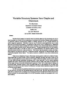
2.2 Initial results and theories Initial analysis of results was based upon the acoustic signatures of each ensemble. As the steady-state spectrum of an organ is essentially harmonic, the acoustic signature plots the amplitude of each harmonic against a third dimension of keyboard range, so that it is possible to view the changes in spectrum between low and high notes. Each of the ensembles had ten samples taken across the keyboard range (each C and F-sharp) which were then analyzed using a Fast Fourier Transform (4096 point Hamming window) and a custom Matlab script to generate harmonic strength information. The acoustic signatures for each ensemble are presented in Figs 1 to 6. Common understanding was demonstrated for the words "flutey", "warm" and "thin". The less rigorous tests for "bright" and "clear" also indicated that some common understanding was present. "Full" and "balanced" did not demonstrate common understanding in this context, and were excluded from further study. The simple theories developed from observation of the acoustic signatures are presented in Disley & Howard (2003), but a more precise means of identifying correlation between test subjects’ ratings and particular spectral features was desired.
TMH-QPSR, KTH, Vol. 46, 2004
St. Chad's 842
60
Amplitude (dB)
50 50-60 40-50 30-40 20-30 10-20 0-10
40 C F#
30 c 20
f# c1 f#1 Pitch
10
c2
f#3 32
30
26
28
24
Harmonics
22
18
c3 20
16
14
10
12
6
8
2
f#2 4
0
0
Figure 1. Acoustic signature for the St Chad’s ensemble (without mixture).
St. Chad's 842M
60
Amplitude (dB)
50 50-60 40-50 30-40 20-30 10-20 0-10
40 C F#
30 c f#
20
c1 f#1 Pitch
10
c2
f#3 32
30
28
24
26
22
20
16
Harmonics
c3 18
14
10
12
6
8
4
f#2 2
0
0
Figure 2. Acoustic signature for the St Chad’s ensemble with mixture.
Speech, Music and Hearing, KTH, Stockholm, Sweden TMH-QPSR, KTH, Vol. 46: 25-40, 2004
27
Disley AC & Howard DM: Spectral correlates of timbral semantics .....
Doncaster 884T2C
60
Amplitude (dB)
50
40 C F#
30
50-60 40-50 30-40 20-30 10-20 0-10
c 20
f# c1 f#1 Pitch
10
c2
f#3 32
30
28
26
24
Harmonics
22
18
c3 20
16
14
10
12
8
4
6
f#2 2
0
0
Figure 3. Acoustic signature for the Doncaster Parish Church ensemble. Jack Lyons 842M
60
Amplitude (dB)
50
40 C F#
30 c 20
f# c1 f#1 Pitch
10
c2
28
f#3 32
30
28
Harmonics Figure 4. Acoustic signature for the Jack Lyons ensemble.
26
24
22
18
c3 20
16
14
10
12
8
4
6
f#2 2
0
0
50-60 40-50 30-40 20-30 10-20 0-10
TMH-QPSR, KTH, Vol. 46, 2004
Heslington 842M
60
Amplitude (dB)
50
40 C F#
30
50-60 40-50 30-40 20-30 10-20 0-10
c 20
f# c1 f#1 Pitch
10
c2 0
f#3 32
30
28
24
26
Harmonics
22
20
16
c3 18
14
10
12
8
4
6
2
0
f#2
Figure 5. Acoustic signature for the Heslington ensemble. Port Sunlight 842M
60
50
Amplitude (dB)
40
50-60 40-50 30-40 20-30 10-20 0-10
30
20
10
F# f#
f#3 32
30
28
26
24
22
20
Harmonics
18
f#2 16
14
12
10
8
6
4
f#1 Pitch 2
0
0
Figure 6. Acoustic signature for the Port Sunlight ensemble. .
Speech, Music and Hearing, KTH, Stockholm, Sweden TMH-QPSR, KTH, Vol. 46: 25-40, 2004
29
Disley AC & Howard DM: Spectral correlates of timbral semantics .....
The two samples from St Chad’s were in a particularly reverberant acoustic, and it was suggested in [3] that this could be partly responsible for the perception of some timbral qualities. Subsequent analysis also revealed that while for most words there was no significant difference between subjects when divided by age or geography (as stated in Disley & Howard, 2003), a minority of words did have significant differences between United States and United Kingdom listeners. Both these issues will be examined in section four.
3. Identification of potential spectral correlates Simple examination of harmonic strength data cannot easily identify or quantify more complex spectral features. There is an established library of spectral features used in similar experiments with single source sounds, but some of these are inappropriate for use in analysis of more complex multi-source ensembles. One particular problem is that of onset and offset transients, as multiple sources will have multiple individual transients that combine into one ensemble transient. It is difficult to apply measures such as DPAT (Duration of Perceived Attack Time) to such a transient, and thus the analyses here will concentrate on the steady state portion of the ensemble sound. This does not imply that the transient portions are perceptually less important, although they can be greatly masked and modified by the acoustic environment in which the ensemble is placed. The analyses described in this section were applied to all six samples used in the experiments described in section two, although only the four samples used in the specialized listening experiment were used in section 3.3.
3.1 Application of existing measures Several existing steady-state measures are easy to adapt to this context. The most common spectral feature mentioned in the theories summarized in section 2.1 is the spectral centroid. This is the mid-point of spectral energy, and the formula used here is given in equation 1.
30
The division by F1 , the fundamental frequency, 32
∑F A n
n =1
32
n
F1 ∑ An
(1)
n =1
results in a normalized centroid that can be directly compared for all ten sample points of each ensemble. Other measures that can easily be applied to each sample are spectral smoothness, spectral slope and average harmonic strength. Spectral smoothness is an average of the absolute difference in amplitude between each harmonic and the next, measured in decibels. Spectral slope is the difference between the lower and higher halves of the spectrum, and average harmonic strength is self-explanatory. Both are again measured in decibels. As most of the change in spectral slope takes place in the central portion of each harmonic analysis, it is also interesting to examine the inter-quartile spectral slope, which excludes the potential padding of the lowest and highest harmonics. Analyses of each spectral feature are presented in Figs 7 to 11. It is not surprising that the mid-twentieth century Neo-Classical ensemble of the Jack Lyons has one of the highest spectral centroids throughout, and the early-twentieth century Romantic ensemble of Port Sunlight has one of the lowest. Doncaster, a century older than the Jack Lyons, is overall its closest match. The zigzagging around the center is mostly due to the way mixtures break back at certain points. Figure 8 shows that the ensemble with the highest centroid is not necessarily the one with the strongest harmonics. The y-axis scale on this and other graphs in this section does not start at zero, to permit presentation of only significant data. Figure 9 displays the way spectral smoothness changes over the keyboard range. A low score represents a smoother transition. Overall, the Jack Lyons is the least smooth ensemble, but things are less clear for all ensembles among the highest pitches.
TMH-QPSR, KTH, Vol. 46, 2004
13 12 11
Normalised centroid
10 9
Doncaster Jack Lyons St Chad (mix) Heslington St Chad (no mix) Port Sunlight
8 7 6 5 4 3 2 C
F#
c
f#
c1
f#1
c2
f#2
c3
f#3
Pitch
Figure 7. Normalised spectral centroids.
22
Average harmonic strength
20
18
16
St Chad (mix) Doncaster St Chad (no mix) Jack Lyons Heslington Port Sunlight
14
12
10
8
6 C
F#
c
f#
c1
f#1
c2
f#2
c3
f#3
Pitch
Figure 8. Average harmonic strength.
Speech, Music and Hearing, KTH, Stockholm, Sweden TMH-QPSR, KTH, Vol. 46: 25-40, 2004
31
Disley AC & Howard DM: Spectral correlates of timbral semantics .....
Difference between harmonic amplitudes
20
18
16
14
Doncaster Jack Lyons Heslington St Chad (mix) St Chad (no mix) Port Sunlight
12
10
8
6
4 C
F#
c
f#
c1
f#1
c2
f#2
c3
f#3
Pitch
Figure 9. Spectral smoothness.
17
15
Amplitude difference
13 Port Sunlight St Chad (no mix) Doncaster
11
Jack Lyons St Chad (mix) Heslington
9
7
5
3 C
F#
c
f#
c1
f#1
Pitch
Figure 10. Spectral slope.
32
c2
f#2
c3
f#3
TMH-QPSR, KTH, Vol. 46, 2004 29
27
Amplitude difference
25
23
Port Sunlight St Chad (no mix) St Chad (mix)
21
Doncaster Jack Lyons Heslington
19
17
15
13 C
F#
c
f#
c1
f#1
c2
f#2
c3
f#3
Pitch
Figure 11. Inter-quartile spectral slope. Figures 10 and 11 respectively display spectral and inter-quartile spectral slope for all six ensembles, where a lower score represents a shallower spectral slope. All of the graphs in figures 7 to 11 have noticeable differences at the highest frequencies. This is probably because the Nyquist frequency is sufficiently low to omit, for example, the fourth harmonic of the Fifteenth 2’ component in each ensemble for f#3, but may also be because the pipes in that octave are harder to regulate due to their small size. As notes in this octave were also not used in the musical examples played to subjects, the upper two samples will be omitted from the search for spectral correlation.
3.2 Development of new measures As each ensemble has only a single numerical rating for each adjective, it is necessary to reduce the measures in section 3.1 above to single quantities before correlation can be looked for. A simple result for each measure can be found by averaging the ten samples, but this removes information on how the measure varies across the keyboard range. Some spectral features tail off as the keyboard ascends, and this can be measured by looking at the difference between the averages of the upper and lower four samples. A measure to complement this is spectral consistency, the
Speech, Music and Hearing, KTH, Stockholm, Sweden TMH-QPSR, KTH, Vol. 46: 25-40, 2004
average difference between each individual sample’s value. Other features do not show such consistent trends, and here it is appropriate to look instead at their standard deviation. Twelve measures are therefore proposed for potential steady-state analysis of ensembles such as the principal chorus of the pipe organ: the average spectral centroid, its fall-off and consistency; the average harmonic strength, its fall-off and consistency; average spectral smoothness and its standard deviation, the average spectral slope and its standard deviation, and the average inter-quartile spectral slope and its standard deviation. Values calculated for these measures from the six organ ensembles can be found in Table 1, where Normalized Frequency Units is abbreviated to NFU. The Pearson correlation coefficients for these twelve spectral measures are presented in Table 2, with correlation significant at the 5% level marked in bold. Several of the measures are significantly correlated here, but this does not mean that they would be correlated for a different set of samples, or outside the context of the pipe organ principal ensemble. At this point many psychoacoustic studies implement a Principal Components Analysis (PCA, details of which can be found in Manly (1994). While such reduction in data sets has
33
Disley AC & Howard DM: Spectral correlates of timbral semantics .....
Table 1. Values of potential spectral components. Potential spectral components
Jack Lyons 8.751
Heslington
Doncaster
Spectral centroid (NFU)
Port Sunlight 6.184
8.424
St Chad (mixture) 8.233
St Chad (no mixture) 6.979
7.654
Centroid fall-off (NFU)
3.395
4.359
4.194
5.091
3.813
3.030
Centroid consistency (NFU)
1.019
0.965
1.264
1.104
1.561
0.646
10.160
14.303
12.685
14.216
16.249
13.684
Strength fall-off (dB)
3.445
3.895
3.050
4.648
5.568
4.563
Strength consistency (dB)
1.329
1.199
0.940
1.926
2.271
1.536
Spectral smoothness (dB)
6.710
14.594
11.546
12.105
10.718
10.183
Standard deviation of spectral smoothness Average spectral slope (dB)
1.883
3.168
3.783
4.943
2.973
2.859
17.930
19.359
19.370
20.059
23.289
22.628
Standard deviation of spectral slope
2.739
1.976
2.525
2.823
2.600
2.754
Average inter-quartile spectral slope (dB) Standard deviation of inter-quartile spectral slope
5.965
7.978
7.336
9.471
11.009
9.193
3.302
2.038
1.786
2.550
3.017
3.823
Average harmonic strength (dB)
Table 2. Correlation between potential spectral components. Centroid
Fall-off
Consist.
Strength Fall-off
Consist.
Smooth
Std. Dev. Spec. Slope
Std. Dev.
IQSS
Std. Dev.
Centroid
1
0.749
0.368
0.790
0.375
0.277
0.912
0.666
Fall-off
0.749
1
0.346
0.302
0.001
0.098
0.635
0.845
0.235
-0.537
0.566
-0.615
-0.281
-0.204
0.159
-0.733
Consist.
0.368
0.346
1
0.392
0.272
0.405
0.049
0.170
0.154
-0.020
0.342
-0.397
Strength
0.790
0.302
0.392
1
0.794
0.645
0.633
Fall-off
0.375
0.001
0.272
0.794
1
0.946
0.112
0.427
0.775
-0.225
0.929
-0.107
0.145
0.837
0.230
0.926
0.444
Consist.
0.277
0.098
0.405
0.645
0.946
1
-0.067
0.179
0.679
0.410
0.830
0.430
Smooth
0.912
0.635
0.049
0.633
0.112
-0.067
1
0.612
0.122
-0.687
0.355
-0.660
Std. Dev.
0.666
0.845
0.170
0.427
0.145
0.179
0.612
1
0.062
0.089
0.392
-0.514
Spec. Slope
0.235
-0.281
0.154
0.775
0.837
0.679
0.122
0.062
1
0.204
0.891
0.446
Std. Dev.
-0.537
-0.204
-0.020
-0.225
0.230
0.410
-0.687
0.089
0.204
1
0.139
0.594
IQSS
0.566
0.159
0.342
0.929
0.926
0.830
0.355
0.392
0.891
0.139
1
0.191
Std. Dev.
-0.615
-0.733
-0.397
-0.107
0.444
0.430
-0.660
-0.514
0.446
0.594
0.191
1
the benefit of simplifying analysis, it removes resulting theories of correlation from direct association with spectral features. Some studies (e.g. Creasey, 1998) dispute the discarding of allegedly less important information as a flawed methodology in the area of psychoacoustics, given the difficulty in isola ting acoustic factors and the complex interaction of perception. A PCA will therefore not be carried out, as its
34
implementation would not contribute to the aims of this experiment.
3.3 Development of spectral correlation theories Table 3 presents the results for each organ on the adjective rating scales for all subjects, expressed as a percentage of maximum possible bias. The words full and balanced have been excluded due to a lack of common
TMH-QPSR, KTH, Vol. 46, 2004
understanding. There was no significant correlation between subject answers for these three words. Table 3. Test results from specialized listeners. Pipe organ ensemble Heslington
Thin
Flutey
Warm
3.64%
-1.82%
-4.85%
Jack Lyons
26.67%
-32.73%
-49.09%
St Chad’s Port Sunlight
-10.61% -19.70%
-0.61% 35.15%
20.91% 33.03%
These answers were compared with the values for the four appropriate samples from Table 1. The Pearson correlation coefficients between the adjectives with common understanding and all spectral analyses developed in sections 3.1 and 3.2 can be found in Table 4. Correlation significant at the 5% level is shown in bold. Ensembles described as "thin" correlate with a large fall-off in spectral centroid across the keyboard range, a less smooth spectrum and a consistent spectral slope. There is a tendency towards a higher spectral centroid, but this is below the level of statistical significance. Ensembles described as "flutey" and "warm" correlate with less fall-off in the spectral centroid, a smoother spectrum (particularly in the case of "flutey") and a less consistent spectral slope. "Flutey" correlates with a lower spectral centroid, and "warm" tends towards this, but again below the level of statistical significance.
The results from the large-scale listening test were more difficult to analyze in this manner. The adjective "bright" was consistently applied to the ensemble with the higher spectral centroid, even when that increase was achieved by adding a mixture stop with a seventeenth component. A seventeenth or Tierce speaks at the fifth harmonic, perceptually adding a reedy quality to the sound (Howard & Angus, 2001). The adjective "clear" was less consistently applied, with significant differences between organists and non-organists. Organists applied the term "clear" to the organ in a less reverberant acoustic, whereas non-organists did not.
4. Verification of theories by synthesis This section aims to verify the correlation theories suggested by the results in section 3.3 and establish firm theories for the words "bright" and "clear".
4.1 Synthesis methodology Synthesis was performed on an electronic organ utilizing the Bradford synthesis system (Comerford, 1993). To maintain relevance to the context of real-world pipe organ ensembles, the sound was processed through a Yamaha SREV-1 convolution-based reverberation unit. It was intended to synthesize several ensembles with different characteristics and take note samples for analysis as in section
Table 4. Correlation between spectral analyses and timbral adjectives. Spectral analysis Spectral centroid Spectral centroid fall-off Spectral centroid consistency Average harmonic strength Average harmonic strength fall-off Average harmonic strength consistency Average spectral smoothness Standard deviation of spectral smoothness Spectral slope Standard deviation of spectral slope Inter-quartile spectral slope Standard deviation of inter-quartile spectral slope
Speech, Music and Hearing, KTH, Stockholm, Sweden TMH-QPSR, KTH, Vol. 46: 25-40, 2004
Flutey -0.952 -0.930 0.044 -0.670 -0.166 0.091 -0.996 -0.700 -0.275 0.913 -0.403 0.722
Adjective Thin 0.775 0.929 -0.382 0.352 -0.178 -0.423 0.941 0.617 -0.097 -0.969 0.040 -0.811
Warm -0.747 -0.907 0.431 -0.314 0.201 0.442 -0.923 -0.574 0.139 0.976 0.000 0.790
35
Disley AC & Howard DM: Spectral correlates of timbral semantics .....
Table 5. Spectral centroid, slope and smoothness data for the four synthesized ensembles. Spectral analysis Spectral centroid (Hz) Spectral slope (dB) Spectral smoothness (dB)
Sample analyzed 842 1609 12.895 2.047
3, but due to unreliable equipment this was not possible. Instead, ensembles were synthesized by means of addition and subtraction of stops. A basic ensemble of principals at 8’, 4’ and 2’ pitch was created (abbreviated to 842 hereafter). A second ensemble with the addition of a mixture provided an increase in spectral centroid (abbreviated to 842M). It was not clear whether any correlation with centroid values was due to the addition of higher frequencies or the omission of lower frequencies. Previous theories about the word "clear" also suggested lower frequencies played a role. A third ensemble was created with a stopped flute instead of a principal as the 8’ component. The 4’ and 2’ remained principals, resulting in a principal ensemble with weaker fundamental and lower harmonic components (abbreviated to S842). Finally, the suggestion in section 3.3 that the acoustic environment played a part in the perception of certain timbral qualities was tested by the use of two different settings on the SREV-1. All three samples were initially presented using preset "Warm Wooden Church no. 1", but the basic principal ensemble was also presented using preset "St John the Divine no. 3" (abbreviated to 842 (rev)). The intention here is not to quantify the effect of a reverberant environment, which would require many more samples and consideration of the many factors affecting acoustic environment, but to investigate whether the acoustic environment has a demonstrable effect on the use of timbral adjectives.
4.2 Application of measures to general spectral data The synthesis equipment failed completely after test examples were created, resulting in an inability to create note samples for analysis. It was therefore impossible to create analyses of variation over the keyboard range. The final
36
S842 1665 12.436 2.143
842M 2301 17.039 2.752
842 (rev) 1459 14.515 2.116
chord of the musical extracts created was analyzed using another custom Matla b script, based on a Fast Fourier Transform with a 8192 point Hamming window, to create comparative measures of spectral centroid, spectral slope and spectral smoothness. As this chord contained multiple notes, the resulting measures are not comparable with those in the previous section, and the spectral centroid is not normalized. The resulting analyses for the four ensembles are presented in Table 5. The desired alterations in spectral centroid have been achieved, although it is interesting to note the effect on those analyses of the different acoustic environments.
4.3 Results from listener tests Sixteen English speaking listeners (eight from the UK, seven from the US and one from Canada) participated in a second comparative listening test, using the five remaining timbral adjectives ("bright", "clear", "flutey", "thin" and "warm") as rating scales for the four synthesized pipe organ ensemble samples. Listener numbers for this and all tests were in line with the recommendations in (Levitin, 1993). Independent listener comments suggested that the illusion of reality had been maintained until test debriefing, confirming result relevance in to real-world contexts. The results are presented in Table 6, with ratings again expressed in terms of a percentage of maximum possible bias. Subsequent analysis by age and geography revealed differences for some adjectives. All listeners were agreed on the most "thin" sample, but disagreed on other words. Although all listeners agreed on the order of samples for the term "clear", UK listeners used the scales to a greater degree than US listeners (43.33% maximum deviation compared with 6.67% for US listeners). Apart from these differences, the results for all other adjectives
TMH-QPSR, KTH, Vol. 46, 2004
Table 6. Overall results of final experiment for all sixteen subjects. Organ ensemble 842 S842 842M 842 (rev)
thin -11.67% 29.17% -5.00% -12.50%
flutey 12.92% 2.50% -37.08% 21.67%
Adjective bright -17.92% -7.50% 57.08% -31.67%
showed high correlation between the groups, demonstrating common understanding.
warm 14.58% -8.33% -32.92% 26.67%
clear -2.08% -0.83% 24.58% -21.67%
previous theories described in von Bismarck (1974), Dodge (1985), Campbell (1994) and Risset & Wessel (1999), although it has not been possible to discern between spectral width and spectral centroid in this context.
4.4 Refinement of spectral correlation theories The Pearson correlation coefficients between the five timbral adjectives from Table 6 and the spectral analyses from Table 5 are presented in Table 7. Correlation significant at the 5% level is marked in bold. Most adjectives demonstrate high correlation with the spectral centroid, but the lack of correlation between the five adjectives (only "bright" and "clear" show significant negative correlation) suggests that the centroid is not the sole factor determining their use. "Bright" and "flutey" appear to have the closest relationship with the spectral centroid. Spectral slope lacks significant correlation with any adjective. Spectral smoothness, which has a significant correlation with the spectral centroid, follows that factor in all cases but with a lower level of significance. The theories for each adjective will be considered individually.
4.4.2 "Clear"
4.4.1 "Bright"
4.4.3 "Flutey"
"Bright" maintains a very clear correlation with the spectral centroid, and also seems to be a significant opposite of "flutey" in this context. It is possible that "flutey" was being used as a synonym for "dull", which was one of the 92 words used less frequently in initial word gathering. This result matches the
"Flutey" is not an obviously useful descriptive term for a pipe organ ensemble, and has no previous research, but has demonstrated consistent common understanding. "Flutey" is negatively correlated with spectral centroid and spectral smoothness.
"Clear" exhibits significant correlation with a higher spectral centroid. This does not support Ethington & Punch (1994), but appears to support Solomon (1959). Jeans (1961) suggested that clarity was related to the strength of lower harmonics, but direct comparison of the 842 and S842 examples resulted in little difference in perceived clarity. This suggests that in the context of the pipe organ clarity is not related to the strength of the lower harmonics. The addition of a mixture improved the perception of "clear", but UK listeners supported this to a greater extent than US listeners. When the 842 and 842 (rev) samples were compared, UK listeners thought that the 842 (rev) sample was less "clear", but US listeners did not perceive a difference between the two samples.
Table 7. Correlation between timbral adjectives and spectral analyses. Spectral analysis
Adjective bright
clear
flutey
thin
warm
0.955 0.568
-0.994 -0.740
0.002
Spectral slope
0.999 0.769
-0.442
-0.928 -0.545
Spectral smoothness
0.966
0.846
-0.958
-0.082
-0.857
Spectral centroid
Speech, Music and Hearing, KTH, Stockholm, Sweden TMH-QPSR, KTH, Vol. 46: 25-40, 2004
37
Disley AC & Howard DM: Spectral correlates of timbral semantics .....
4.4.4 "Thin" "Thin" showed a tendency in Table 4 towards correlation with a higher spectral centroid, but it was unclear whether this was due to the presence of higher harmonics or the lack of lower harmonics. The results presented in Table 6 clearly suggest that a reduction in lower harmonics is responsible for perceived "thinness". When the mixture was added, despite a much greater increase in the spectral centroid, the ensemble was perceived as less thin. There was disagreement between the UK and US listeners on whether the presence of higher harmonics contributed to "thinness", but all subjects agreed that the lack of lower harmonics was far more important. In the synthesis experiment, "thin" did not significantly correlate with any spectral analysis, despite the previous strong negative correlation with a smooth spectrum in Table 4.
4.4.5 "Warm" "Warm" correlates with a lower spectral centroid, but to a lesser extent than "flutey". In previous research (Ethington & Punch, 1994; Pratt & Doak, 1976) "warm" was rela ted to a decrease in spectral centroid and an increase in the strength of the first few harmonics. This latter quality is impossible to measure from the complex chords analyzed in section 4.2, but in the test directly comparing the 842 and S842 samples, of which the latter had reduced lower harmonics, the former was considered warmer overall by an average of 15%. The theory of decreased spectral slope also suggested in Syrový et al. (2003) is partially supported as the correlation between slope and perceived warmth is consistently negative, but this is well below the level of statistical significance.
4.4.6 The effect of acoustic environment on timbral adjectives used The aim of this part of the experiment was not to quantify the effect of acoustic environment, but demonstrate that it can have an effect on the timbral adjectives used to describe otherwise identical sources. Reverberation is not a simple linear quantity as might be implied by such measures as RT60 , but can also have a spectral filtering element. In the example of increased reverberation used in this section, there is a marked reduction in the spectral centroid and an increase in the spectral slope (see Table 5). It is possible that a differnet reverberant environment would
38
provide an equivalent increase in RT60 without the same spectral effect, due to the presence of different sound-reflecting and absorbing materials. Within those constraints, the effect of the alteration in reverberant environment on the timbral adjectives studied in this section can be examined. "Thin" was the subject of some disagreement, resulting in an overall neutral result that concealed the differences of opinion. The reverberant example was perceived as less "bright" than the less reverberant example, which might be expected from its reduction in spectral centroid. US listeners felt that the addition of reverberation added to the perception of "warm", whereas UK listeners felt it decreased the perception of "clear". Both these adjectives are related to the spectral centroid in a way that does not make this difference entirely inconsistent. All listeners agreed on an increased perception of "flutey" when reverberation was added.
5. Conclusions This paper has examined the timbral adjectives used by specialized listeners to describe complex multi-source ensembles, and has developed a series of steady-state analyses suitable for detailed analysis of such ensembles. Despite problems in verification of some theories, correlation has been found between some timbral adjectives and spectral features. Within the context of English speakers describing the principal ensemble of a pipe organ, listeners describing a sound as "thin" will be referring to a comparative lack in strength of the lower harmonics. A "flutey" ensemble will have a lower spectral centroid, as will a "warm" ensemble. A "bright" ensemble will have a higher spectral centroid, as will a "clear" ensemble. Such an ensemble placed in a more reverberant environment may be considered more "flutey" and "warm", the latter particularly the case with US listeners. UK listeners thought that the more reverberant environment made the ensemble less "clear".
6. Acknowledgements The authors gratefully acknowledge the University of York for providing funding and equipment for this study. Thanks are also due to the volunteer listeners from the University
TMH-QPSR, KTH, Vol. 46, 2004
of York and members of the Internet mailing list piporg-l, as well as the churches, organizations and their staff who facilitated recordings of their pipe organs.
7. References Anderson P-G (1969). Organ Building and Design, George Allen and Unwin. Campbell SL (1994). Uni- and multidimensional identification of rise time, spectral slope, and cutoff frequency, JASA 96/3: 1380-1387. Comerford PJ (1993). Simulating an organ with additive synthesis, Computer Music Journal, 17/2: 55-65. Creasey DP (1998). An exploration of sound timbre using perceptual and time-varying frequency spectrum techniques, DPhil thesis, unpublished, The University of York, p 48. Disley A C & Howard DM (2003). Timbral semantics and the pipe organ, Proceedings of the Stockholm Music Acoustic Conference 2003, 607610. Dodge C & Jerse TA (1985). Computer Music: Synthesis, Composition and Performance, Schirmer Books. Ethington R & Punch B (1994). SeaWave: A system for musical timbre description, Computer Music Journal, 18/1: 30-39. Hall DE (1991). Musical Acoustics, Brooks/Cole Publishing, 2nd ed.. Howard DM & Angus J (2001). Acoustics and Psychoacoustics, Focal Press, 2nd ed., p 222. Jeans J (1961). Science and Music, Cambridge University Press. Levitin DJ (1993). Experimental Design in Psychoacoustic Research, Music, Cognition and Computerized Sound, ed. Cook PR, MIT Press, 299-327. Manly BFJ (1994). Multivariate Statistical Methods: A Primer, Chapman and Hall, London, 2nd ed. Nykänen A & Johansson Ö (2003). Development of a language for specifying saxophone timbre, Proceedings of the Stockholm Music Acoustic Conference 2003, 647-650. Owen B & Williams P (1988). The Organ, New Grove, Macmillan. Pierce JR (1983). The Science of Musical Sound, Scientific American Books, New York. Pratt RL & Doak PE (1976). A subjective rating scale for timbre, Journal of Sound and Vibration, 43/3: 317-328. Rioux V (2001). Sound Quality of Flue Organ Pipes – An Interdisciplinary Study on the Art of Voicing, PhD thesis, Chalmers University of Technology, Sweden. Risset J-C & Wessel DL (1999). Exploration of Timbre by Analysis and Synthesis, The Psychology of Music, ed. Deutsch D, Academic Press, 2nd ed.
Speech, Music and Hearing, KTH, Stockholm, Sweden TMH-QPSR, KTH, Vol. 46: 25-40, 2004
Risset J-C & Matthews MV (1969). Analysis of musical instrument tones, Physics Today, 22/2: 23-30. Rossing TD (1990). The Science of Sound, Addison-Wesley. Solomon LN (1959). Search for physical correlates to psychological dimensions of sounds, JASA 31/4: 492-497. Syrový V, Otcenášek Z & Štepánek J (2003). Subjective evaluation of organ pipe timbre in the standard listener positions, Proceedings of the Stockholm Music Acoustic Conference 2003, 333336. von Bismarck G (1974). Sharpness as an attribute of the timbre of steady sounds, Acustica 30/3: 159-172.
39
Disley AC & Howard DM: Spectral correlates of timbral semantics .....
40