Spectral correlations in systems undergoing a transition from ...

PHYSICAL REVIEW E

VOLUME 59, NUMBER 6

JUNE 1999

Spectral correlations in systems undergoing a transition from periodicity to disorder T. Dittrich Departamento de Fı´sica, Universidad de los Andes, A.A. 4976, Santafe´ de Bogota´, Colombia

B. Mehlig Theoretical Physics, University of Oxford, Oxford, United Kingdom

H. Schanz Max-Planck-Institut fu¨r Stro¨mungsforschung, Bunsenstrasse 10, 37073 Go¨ttingen, Germany

Uzy Smilansky Department of Physics of Complex Systems, The Weizmann Institute of Science, Rehovot 76100, Israel

Pe´ter Pollner and Ga´bor Vattay Department of Physics of Complex Systems, Eo¨tvo¨s University, Box 32, H-1518 Budapest, Hungary ~Received 25 November 1998! We study the spectral statistics for extended yet finite quasi-one-dimensional systems, which undergo a transition from periodicity to disorder. In particular, we compute the spectral two-point form factor, and the resulting expression depends on the degree of disorder. It interpolates smoothly between the two extreme limits—the approach to Poissonian statistics in the ~weakly! disordered case, and the universal expressions derived in T. Dittrich, B. Mehlig, H. Schanz, and U. Smilansky, Chaos Solitons Fractals 8, 1205 ~1997!; Phys. Rev. E 57, 359 ~1998!; B. D. Simons and B. L. Altshuler, Phys. Rev. Lett. 70, 4063 ~1993!; and N. Taniguchi and B. L. Altshuler, ibid. 71, 4031 ~1993! for the periodic case. The theoretical results agree very well with the spectral statistics obtained numerically for chains of chaotic billiards and graphs. @S1063-651X~99!11005-5# PACS number~s!: 05.45.2a, 03.65.Sq

I. INTRODUCTION

The spectrum of an unbounded periodic system is arranged in continuous bands and the corresponding eigenfunctions are extended ~unnormalizable!. When sufficient disorder is introduced, the system is Anderson localized— the spectrum is pointlike and the eigenfunctions are localized ~normalizable!. The transition from a continuous to a point spectral measure is a drastic effect, which might have been used to characterize the transition. However, this approach is of a limited value, since in practice one always deals with finite systems, where the spectral measure is pointlike both in the periodic and in the disordered situations. In finite systems, the mean spectral density is independent of the degree of disorder. Therefore, for finite systems, the effect of disorder on the energy spectrum can be discerned only in the spectral correlations. Indeed, this approach to the characterization of the Anderson transition in three-dimensional systems was used @1#, and the spectral measures were shown to undergo an abrupt change when the critical level of disorder is reached. In the present paper we study the spectral statistics for finite quasi-one-dimensional ~Q1D! systems, which undergo a transition from periodicity to disorder. ~Q1D disordered systems of finite length can be either ‘‘metallic’’ or ‘‘insulating’’ depending on whether the localization length is larger or smaller than the system length. We shall consider only the first case, and the strength of the disorder will be restricted accordingly, to the range of values which is sometimes called weak disorder.! We shall focus our attention to the spectral two-point form factor, and show that it depends 1063-651X/99/59~6!/6541~11!/$15.00

PRE 59

very sensitively on the degree of disorder, and derive a universal expression, which interpolates continuously between the periodic and the disordered yet metallic limits. Scaling theory describes the transition from metallic to insulating behavior by varying just a single parameter, the dimensionless conductance c. Here, in contrast, we encounter two independent parameters characterizing the disorder. The role of the conductance is played by the classical diffusion constant D that remains finite even in the case of exact periodicity. Disorder, in the sense of a breaking of spatial symmetry, will be characterized independently by the deviation of the classical periodic orbits from N-fold degeneracy ~where N is the number of unit cells!. The presence of two disorder parameters reflects that we are here simultaneously dealing with dynamical ‘‘disorder’’ ~chaos! and spatial ~quenched! disorder. The transition regime we are considering is therefore outside the scope of any one-parameter scaling theory. The study of the spectral fluctuations in the transition from periodicity to disorder is relevant for various theoretical and experimental endeavors to characterize the transition to localization. On the one hand, it provides a new and very sensitive theoretical and computational tool. On the other hand, it offers the basis for the extension of the microwave measurements of the Marburg group @2#, who measured the spectral distribution of a periodic cavity, and are now in the process of introducing disorder. The spectral form factor is the main object of our discussion, and it is defined in the following way. The spectrum is unfolded by introducing the dimensionless energy e , through 6541

©1999 The American Physical Society

T. DITTRICH et al.

6542

the relation d e 5 ^ d & (E)dE, where ^ d & (E) is the mean spectral density. The corresponding dimensionless time t measures time in units of the Heisenberg time t H 52 p \ ^ d & . We consider a finite spectral interval of length D e centered at e c , and denote its characteristic function by x ( e 2 e c ). Since the mean spectral density of the unfolded spectrum is unity, the number of states in the interval D e is N5D e . This energy interval should be sufficiently large so that N@1, and sufficiently small so that the mean level density and the classical dynamics do not change much as the energy is scanned across it. The oscillatory part of the spectral density in this interval is ˜d ~ e ! 5 x ~ e 2 e c !

F( q

G

d ~ e 2 e q ! 21 .

5

E

e

K~ t !5

22 p i et˜

d~ e !de

(q x ~ e q 2 e c ! e 22 p i e t 2 d D t~ t ! . q

~2!

The Fourier transform of the normalized characteristic function is denoted by d D t ( t ) and its width is D t ;1/D e . The form factor is expressed as K~ t !5

1 ^u d ~ t !u 2& c . N c

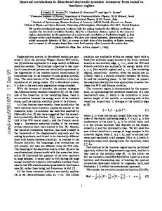
FIG. 1. Periodic ~a! and aperiodic ~b! chains of chaotic billiards. The chain length is denoted by L; a is the size of an individual billiard. Thus N5L/a is the number of units in the chain.

~1!

The Fourier transform of this function is d c~ t ! 5

PRE 59

~3!

We use ^ & c to denote the spectral average, which is taken over the nonoverlapping energy intervals located about a set of e c values. One can also perform the averaging over any free parameter of the system or over disorder when it is introduced. It can be easily shown that Eq. ~3! is merely the Fourier transform of the spectral two-point correlation density @3#. For a discrete spectrum the normalization in Eq. ~3! is such that the form factor approaches a constant g as t →`, where g is the mean spectral degeneracy. The expressions for the spectral form factors in the extreme situations of exact periodicity and weak disorder are known. In the latter case, when the length of the system does not exceed the localization length, and assuming that the Heisenberg time is shorter than the Thouless time, the spectral statistics takes the form @4#

H

g T At /2c

for t ,1

1

for t .1.

~4!

The factor g T can take the values 1 or 2 depending on whether time reversal invariance is respected or violated, and c is the conductivity of the chain. The spectral form factor for periodic systems was recently derived using both fieldtheoretical methods @5# and the semiclassical approximation @6#. Since the latter theory is the basis for the approach developed in the present paper, we shall describe it briefly to introduce the concepts and the notations which will be used in the sequel. We consider a chain of N identical chaotic unit cells of length a51, with periodic boundary conditions, such that the full system shows a discrete translation invariance @Fig. 1~a!#. ~Alternatively, we could discuss a disordered ring configuration which is threaded by an Aharonov-Bohm flux line. This is the system analyzed in @5#!. In such a system, the classical evolution within a unit cell becomes ergodic after a short time, and one can approximate the classical evolution in the entire chain by diffusive evolution. We shall denote the diffusion constant by D. The time it takes the diffusive evolution to cover the phase-space uniformly is the Thouless time. Due to translation invariance, the quantum spectrum consists of discretized energy bands whose width depends on the ~dimensionless! conductivity per unit cell. It is defined as c 1 52 p \ ^ d 1 & D/a 2 , where ^ d 1 & is the mean level density per unit cell. A few examples of typical bands are shown in Fig. 2. One can see that for low c 1 , the bands are flat and show little structure. For high values, the bandwidth is of the order of the interband spacing, and the bands can hardly be recognized if the discretization is too coarse.

FIG. 2. Typical discretized band spectra of a periodic chain with N516 unit cells. The energy levels are shown as a function of the Bloch phase u n for 10 bands in the case of ~a! low, ~b! intermediate, and ~c! high conductance.

PRE 59

SPECTRAL CORRELATIONS IN SYSTEMS UNDERGOING . . .

If the system under discussion is invariant under an antiunitary symmetry ~such as, e.g., time reversal!, the bands are symmetric about the center and the edges of the Brillouin zone, and the levels are doubly degenerate ( g 52). The reflection symmetry and the degeneracies are broken if the symmetry is lifted, and in this case g 51. The quantum spectrum is characterized by two energy scales, the mean intraband spacing and the mean interband spacing. The ratio between them is at least N, the number of unit cells. We are interested here in the large N limit, and therefore these energy scales are very well separated. Since ^ d & ' ^ d 1 & N, the spectral correlations which pertain to the interband scale affect the behavior of the form factor in the range 0, t ,1/N. The correlations between levels in the same band leave their mark on K( t ) in the domain 1/N, t ,1. The fact that the spectrum is composed of discrete ~possibly degenerate! energy levels is expressed in the spectral form factor in the domain 1, t , where the form factor approaches the constant value g . We used different approximations to express the form factor in the three domains mentioned above @6#. ~i! 0, t ,1/N. Here one starts from the semiclassical trace formula @7# and employs the ‘‘diagonal approximation’’ @8# to write K ~ t ! 'g T N t P ~ t ! .

~5!

The factor N is due to the discrete translation symmetry, because of which any generic periodic orbit is replicated N times in the system. g T stands for the classical degeneracy due to time-reversal ~or any other antiunitary! symmetry and it can take the values 1 or 2. P(t) is the classical probability to stay in the same unit cell from which the trajectory started, after the time t5 t t H @4#. Because phase space is covered diffusively, P(t)'(1/2 p Dt) 1/2 and hence K ~ t ! 'g T N AN t /2c 1 ,

~6!

where c 1 is the dimensionless conductivity per unit cell which was introduced above. ~ii! 1/N, t ,1. As t increases, the form factor provides information on a finer energy scale. In the vicinity of t 51/N, the energy levels within a single band cannot be resolved, hence K( t '1/N) takes a value which is proportional to the apparent degeneracy N. Finer details of the energy correlation inside the band are manifested for larger values of t . To understand the behavior of the spectral form factor, one writes the levels in the band b as e b (q), q51, . . . ,N, and substitutes in Eq. ~3!. Neglecting the cross-band correlations one gets

K U(

1 K~ t !5 N

q51

UL 2

N

e

2i2 p e b (q) t

.

~7!

due to the Van Hove singularities. Denoting by ] 2q e b the second derivative of the band function at its extrema, one gets K ~ t ! 5C ^ ~ ] 2q e b ! 21 & b t 21 ,

~8!

where C is a numerical constant. It was shown in @6# that the values of the constants which appear in Eq. ~6! and in Eq. ~8! are compatible so that the two expressions match at t 51/N. ~iii! t .1: The time interval is sufficient to resolve the pointlike character of the spectrum. Hence, K~ t !5g.

~9!

In the following sections we shall study how the expressions ~6!, ~8!, and ~9! make the transition to the Poisson form factor K( t )51 as disorder is introduced. The semiclassical ~diagonal! approximation will be the starting point for the discussion of the transition in the first domain. This will be done in Sec. II. To investigate K( t ) in the second and the third domains, it suffices to study a system which has a single band in the periodic limit. The N-site periodic Anderson model is such a system, and it will be discussed in Sec. III. The important observation made in this section is that the transition is well described by considering the disorder perturbatively. The resulting explicit formulas for K( t ) in the transition regime reproduce the numerical data extremely well. The perturbative treatment also sheds light on the peculiar mechanism which reduces the value of K( t ) from g to 1 in the third domain when the disorder splits up the degeneracies of the spectrum. We shall compare the results obtained separately for the three domains with numerical data for billiard and graph ~network! systems. This will be done in Sec. IV, where we shall summarize and discuss our findings. II. INTRODUCING DISORDER—THE SEMICLASSICAL APPROXIMATION

We shall compute the spectral form factor ~3! in terms of the Fourier transform of the oscillatory part of the spectral density. Using Gutzwiller’s trace formula, d( t ) can be expressed semiclassically as a sum over the periodic orbits j of the system d~ t !5

(j d D t~ t 2 t j ! t j A j e is

j

~10!

with primitive period t j ' t . A j denotes the weight of the orbit corresponding to its stability and includes the Maslov phase. s j is the action of the orbit in units of \. Following the standard approximation, we neglect the contribution of repetitions of primitive orbits to the sum ~10!. The form factor is now given by a double sum over periodic orbits

b

This is the spectral form factor for a band, averaged over all the bands. The q summation can be performed by the saddlepoint ~or the uniform! approximation. The main contribution comes from the vicinity of the band extrema which correspond to the energy values where the spectral density is singular. That is, the prominent features in the form factor are

6543

K~ t !5

1 De

K(

j, j 8

L

d D t ~ t 2 t j ! d D t ~ t 2 t j 8 ! A j A *j 8 e i(s j 2s j 8 ) . ~11!

It is well known @8# that for short time t this sum can be restricted to the diagonal terms j5 j 8 . However, when due to a symmetry, the orbit appears in g j different but symmetry-

6544

T. DITTRICH et al.

related versions, and the contribution of all the symmetryconjugated orbits must be added coherently. In such cases, Eq. ~11! reduces within the diagonal approximation to K~ t !'

(j g j d D t~ t 2 t j ! t j u A j u 2 .

~12!

In the case of an extended, nearly periodic system, the diagonal approximation is valid up to t 51/N, the Heisenberg time of the unit cell @3#. From very general arguments it is clear that in a system whose phase space decomposes into several equivalent subspaces related by ~unitary as well as antiunitary! symmetry, the mean degeneracy g is just the number of such subspaces. Thus, if time-reversal invariance is the only symmetry obeyed, phase space points with opposite momenta are equivalent and consequently phase-space is partitioned in g T 52 subspaces. In our problem, phase space is invariant under a symmetry group containing N elements and therefore g5Ng T . Using the sum rule for periodic orbits @9,4#, the form factor is finally written as K ~ t ! 'g T N t P ~ t ! ,

~13!

which we introduced in Eq. ~5!. The normalization of the staying probability P( t ) is such that P( t )5V/ v ( t ) at a time t , where the classical flow covers ergodically the part v ( t ) of the total energy-shell volume V. In particular, P( t →`)51 for an ergodic system and P( t )5N in a system which is composed of N unconnected ergodic cells. A more precise definition can be found in @4,10,3#. For the present purpose, we need only the following property @3#: the return probability for a system composed of chaotic unit cells is independent of the presence or absence of long-range spatial order. Thus, within the diagonal approximation, the only effect of the introduction of disorder is the destruction of the coherence between the contributions of orbits which were related by symmetry in the original periodic system. This implies that in the diagonal approximation for K( t ) @see Eq. ~13!#, g5Ng T is to be replaced by g5g T . In order to describe the transition from g5Ng T to g 5g T as the spatial symmetry is broken, we go slightly beyond the diagonal approximation ~12! in that we retain in Eq. ~11! the off-diagonal contributions from all those orbits which are degenerate in the symmetric system, K ~ t ! 'g T

U

N

e i(Ds (r d D t~ t 2 t r ! t ru A ru 2 j,( j 51 8

U

r, j 2Ds r, j 8 )

2

. ~14!

r runs now over all groups of symmetry-related orbits, while j, j 8 label the N orbits within each group. Possible degeneracies due to time reversal are not affected by breaking the spatial symmetry and are thus contained in the prefactor g T . The disorder which breaks the symmetry has been assumed weak enough such that ~i! the orbits within the Heisenberg time of the unit cell t r ,1/N are structurally stable, i.e., no ~short! periodic orbits appear or disappear due to the disorder, and ~ii! the disorder does not alter by much the stability amplitudes and the periods within a group r so that in the prefactor A r, j 'A r , t r, j ' t r . The variation of the actions are

PRE 59

of the same order, but they cannot be neglected because they are measured in units of \ and, therefore, the resulting changes in phase, Ds r, j , should be taken into account. Comparing Eqs. ~12! and ~14! we see that Eq. ~13! represents the form factor also in the case of a weakly broken spatial symmetry, if g is replaced by an effective degeneracy g~ t,d !5

5

gT N

K( S K( N

j, j 8 51

gT N1 N

e i(Ds r, j 2Ds r, j 8 )

jÞ j 8

L

r

e i(Ds r, j 2Ds r, j 8 )

LD

,

~15!

r

which depends on the time t since the average on the righthand side is over all groups of periodic orbits r with length t r ' t . The dimensionless parameter d has been introduced to characterize the strength of the symmetry-breaking disorder in a way to be specified in Eq. ~16! below. In order to evaluate Eq. ~15!, we need some information about the distribution of the disorder contributions to the phases of the periodic orbits Ds r, j . We assume that the correlation length of the disorder is negligibly small compared to the mean length of an orbit. In this case Ds r, j is a sum of many independent contributions, and the number of these contributions is proportional to the period of the orbit t . Hence, according to the central limit theorem, Ds r, j are independent Gaussian random variables with mean value ^ Ds & 50 and variance

^ D 2s & 5 d 2t ,

~16!

where the average is over all orbits of period t . With these assumptions we find, from Eq. ~15!, g~ t,d !5

gT ~ N1N ~ N21 ! u ^ e iDs & u 2 ! N

5g T ~ 11 @ N21 # e 2 d t ! . 2

~17!

In the first line we have used the fact that the N@1 together with the statistical independence of Ds r, j and Ds r, j 8 justified above to replace the sum over j, j 8 by its averaged value. In the second line, the Gaussian distribution of Ds was em2 ployed to give ^ e iDs & 5e 2 ^ D s & /2. It is easy to see that Eq. ~15! indeed interpolates between g5Ng T and g5g T as a function of the disorder. Note that the parameter which characterizes the disorder, d 2 , is multiplied by the time t over which the disorder acts. Hence, the classification of the disorder as ‘‘weak’’ or ‘‘strong’’ depends on the relevant time scale. In summary, we get K ~ t , d ! 5g T ~ 11 @ N21 # e 2 d t ! t P ~ t ! 2

5g T ~ 11 @ N21 # e 2 d t ! AN t /2c 1 ; 2

t ,1/N. ~18!

This expression provides the smooth transition from the periodic case, via the weakly disordered to the ‘‘metallic’’ domain. In Sec. IV we shall show that this simple formula

PRE 59

SPECTRAL CORRELATIONS IN SYSTEMS UNDERGOING . . .

reproduces the form factor in the transition from periodicity to disorder very well. We emphasize once again that the present theory does not describe strongly disordered systems where the localization length is shorter than the system size. Such systems are outside of the scope of the present approach, which is based on the ‘‘diagonal’’ approximation. III. INTRODUCING DISORDER–PERTURBATION OF A MODEL WITH A SINGLE BAND

As explained in the Introduction, the form factor in the domain t .1/N is sensitive to the correlations among the levels which belong to the same band. Therefore, in order to investigate the form factor in this region, it is sufficient to study a model with a single band, which is what we do in the present section. In order to use the results of this section in the general context, we have to remember that the form factor in realistic systems is obtained as an average over many bands @see Eq. ~7!#. This will smooth out several features of the single-band form factor, as will be explained in the sequel. The system we consider is a chain of N unit cells of length a51, with periodic boundary conditions at the end of the chain. The chaotic scattering process in each cell is represented by a random potential and the dynamics is discretized on a lattice. Choosing convenient units, the Schro¨dinger equation reads 2 ~ f n11 22 f n 1 f n21 ! 1V n f n 5E f n ,

f n 5 f N1n , ~19!

where f n is the wave function on the nth site. The on-site potentials V n are uncorrelated random variables which are picked out from the same Gaussian distribution function with variance s . They obey

^ V n & 50,

^ V n V m & 5 d nm s 2 ,

n,m50, . . . ,N21.

~20!

The complexity of the scattering process is incorporated by neglecting the correlations between the potentials on different sites. In the periodic limit ( s 50), the levels are arranged in a discrete band E 0q 52 @ 12cos~ 2 p q/N !# ,

q50, . . . ,N21.

~21!

The level density @compare Eq. ~1!#

(

q50

els can be unfolded with the constant density. Since we consider here only weak disorder, the mean level density is taken as

^ d & 'N/4.

~22!

The spectral form factor was defined in Eq. ~3!. In the periodic case the energies are given by Eq. ~21!. The spectral form factor is K ~ t , s 50 ! 5

1 N

U(

U

N21 q50

2

exp~ 2i p E 0q t N/2! .

~23!

The second argument of the form factor denotes the strength of the disorder, and in the present periodic case it is 0. The expression ~23! can be rewritten by expanding the exponential into a Bessel series: `

e

iN t p cos

S 2 Np q D 5 ( i k e iq(2 p /N)k J k~ p N t ! . k52`

~24!

Exchanging the order of the summation over q and k yields

U

U

`

K ~ t ,0! 5N J 0 ~ p t N ! 12

(

n51

2

i nN J nN ~ p t N ! .

~25!

The function K( t ,0), which is shown in Fig. 3, displays different features in the three domains of t . In the domain 0 < t