Spectral densities of embedded interfaces in

PHYSICAL REVIEW B 70, 144205 (2004)

Spectral densities of embedded interfaces in composite materials A. R. McGurn Department of Physics, Western Michigan University, Kalamazoo, Michigan 49008, USA

A. R. Day Department of Biochemistry, Michigan State University, East Lansing, Michigan 48824-1116, USA

D. J. Bergman School of Physics & Astronomy, Raymond and Beverly Sackler Faculty of Exact Sciences, Tel Aviv University, Tel Aviv 69978, Israel

L. C. Davis and M. F. Thorpe Department of Physics and Astronomy, Michigan State University, East Lansing, Michigan 48824-1116, USA (Received 5 March 2004; published 26 October 2004) The effective resistivity and conductivity of two media that meet at a randomly rough interface are computed in the quasistatic limit. The results are presented in the spectral density representations of the Bergman-Milton formulation for the properties of two-component composite materials. The spectral densities are extracted from computer simulations of resistor networks in which the random interface separates two regions containing different types of resistors. In the limit that the bond lengths in the resistor network are small compared to parameters characterizing the surface roughness, the resistor network simulation approximates the continuum limit of the two-component composite. The Bergman-Milton formulation is used to obtain a set of exact sum rules in the continuum limit for the spectral densities in terms of parameters describing the surface roughness and the simulation results are found to agree with these limiting forms. Perturbation theory results of the composite in the continuum limit for weakly rough random interfaces are also presented. An expansion of the spectral density is determined to second order in the surface profile function of the random interface and compared with the Bergman-Milton sum rules and computer simulation results. The formalism is applied to surface plasmons, electron energy loss, and light scattering from rough surfaces. Layered structures are discussed briefly. DOI: 10.1103/PhysRevB.70.144205

PACS number(s): 41.20.Cv, 71.36.⫹c, 77.55.⫹f, 02.70.Hm

I. INTRODUCTION

The theory of the conductivity and resistivity of composite materials has a long history. Earliest considerations (see, e.g., the book by Sihvola1) were based on simple analytical methods. These emphasized exactly solvable models, perturbation treatments, and effective medium approximations. Modern theories have focused on more sophisticated analytical treatments2–12 and on computer simulations.6–10,13–19 Of particular interest to us in this paper is the formulation of Bergman and Milton, first published in Refs. 3 and 4, and later in greater detail in a lecture notes volume,5 for calculating the conductivity and resistivity properties of twocomponent composite materials. This method is based on a formal solution of Gauss’s Law and has yielded a number of exact inequalities, limiting forms, and sum rules for twocomponent composites. In this “spectral treatment,” the formal solution for the average conductivity and resistivity of the composite system are expressed as functions of the conductivities or resistivities of its two-components in terms of an integral (Hilbert) transform involving a spectral density and a simple pole, or an entire sequence of simple poles in the case of a periodic microstructure. The physics of the solution is in the spectral density which depends on the geometry of the constituent materials of the composite. Once the spectral density is known the effective conductivity and resistivity properties of the system are determined for all 1098-0121/2004/70(14)/144205(22)/$22.50

possible values of the resistivities and conductivities of the two components forming the system. The spectral density is difficult in general to compute and has only been determined exactly for restricted geometries. Some analytical and numerical results are also available in perturbation theory and moment expansions and for special cases.3,4,6–10,13,14,17–23 Although the spectral density in general cannot be calculated by analytical means, developments in computer simulation techniques7,24–30 now allow for the numerical determination of the spectral density.14,18,19,24–28,31 Spectral density methods are found to be of great generality and have been applied to a wide variety of different systems. These include randomly disordered materials,8–10,13,14,18–20,24–28,31 periodically ordered materials,6–10,21–23 and those with isolated impurities of a regular geometry.1,8–10,24,25 Resistor network simulations can greatly facilitate the study of spectral densities of two-component composites.18,19,32 One of the earliest many-body problems treated by means of computer simulations is the resistor network problem.13 This involves the numerical determination of the resistivity of a mixed network of resistors, and is of interest as a model for random alloys, particularly when the length of a resistor in the network is small compared to typical length scales in the alloy. The resistor network problem has interesting transport and phase transition properties, which have led to the development of a number of efficient algorithms for the quick solution of large arrays of mixed

70 144205-1

©2004 The American Physical Society


MCGURN et al.

resistors. These algorithms are now finding application with the Bergman-Milton formulation.18–28,31,32 The first use of resistors arrays to extract the spectral density of twocomponent alloys was in the paper of Day and Thorpe.18 In this paper a general two-dimensional alloy was treated and the features of the spectral density determined for a wide variety of disorders.18,19,32 This spectral density approach was also used to model the optical properties of a twocomponent material.32 Here the Day and Thorpe method is used to determine the continuum limit of the spectral density in the BergmanMilton formulation for the resistivity and conductivity of two media that meet at a randomly rough buried interface. For simplicity, the interface between the two different resistive or conducting media is described by a one-dimensional Gaussian random profile function so that the interface retains translational symmetry along one axis in space.33,34 Generalizations to two-dimensionally rough surfaces can be made, but require much more computational effort.34 The treatment of more general surface roughness statistics is straightforward and the choice of Gaussian random statistics is discussed later in the text. The calculations are for the low frequency limit of the conductivity or resistivity in which the displacement current is ignored, and are done by using a combination of resistor network simulations and analytical techniques. Comparison of the spectral density results from simulation data is made with a variety of analytical limiting forms. The bulk of the results in this paper for the random interface in a two-component composite are obtained from resistor network simulations involving systems with bond disorder. The coordinates of a Gaussian randomly disordered interface are generated and are then used to separate two regions of different resistor types. In the limit that the parameters characterizing the rough interface between the two regions of different resistor bonds are large compared to the bond lengths, the continuum limit is well approximated. The spectral density in the continuum limit is extracted from computer simulation results. The Bergman-Milton theory is used to generate a number of sum rules obeyed by the continuum limit of the spectral density for the interface. (It is important to note, in regard to the Bergman-Milton theory, that the exact sum rules usually apply away from the continuum limit as well. We believe that this is true for the resistor networks studied here.) These results, which are of interest in themselves, are used to check the simulation data. Perturbation theory results for the continuum limit of the interface problem are generated in the limit of weak roughness. The expansion parameter is the surface profile function, which is represented by a set of Gaussian random stationary functions. An expression for the spectral density to second order in the surface profile function is obtained and found to agree with the Bergman-Milton sum rules and the results of the computer simulation. The order of the paper is: In Sec. II, the continuum model is presented and discussed, using a spectral formulation of the Bergman-Milton type, and a number of sum rules are derived. In Sec. III, the computer simulation is discussed. Results for the spectral densities are presented, and a comparison is made with the limiting forms obtained in Sec. II. Perturbation theory for weakly rough interfaces is presented

in Sec. IV. In Sec. V, applications are made to surface plasmons, electron energy, and light scattering from rough surfaces. Generalizations of the theory to treat multiple layered media are in Sec. VI. A general discussion of the results is given in Sec. VII. II. SPECTRAL FORMULATION

Consider a quasistatic system between two parallel plates. The upper z = L / 2 plate is at a potential V0, and the lower z = −L / 2 plate is at zero potential. Between the parallel plates are two media of conductivities ␴1 and ␴2 (resistivities ␳1 and ␳2) separated by a (two-dimensional) interface that is rough in one of its two dimensions. Two geometries are treated: In the first, the average of the rough surface separating the two media is the y-z plane. For this geometry the effective conductivity of the medium between the parallel plates is calculated. In the second, the average of the rough surface separating the two media is the x-y plane. For this geometry the effective resistivity of the medium between the parallel plates is calculated. In both geometries the average electric field is defined by2,6

冕

1 Eជ 0 = V

ជ 共rជ兲d3r, E

共1兲

ជ where Eជ 共rជ兲 is the field between the parallel plates, E 0 = ezV0 / L, and V is the volume between the plates. The effective conductivity ␴ef f of the medium between the parallel plates is then defined by ជ =1 Jជ 0 = ␴ef f E 0 V

冕

Jជ d3r,

共2兲

with the effective resistivity related to ␴ef f by ␳ef f = 1 / ␴ef f . A. Average interface in the y-z plane

In this geometry the position-dependent conductivity of the medium between the parallel plates is given by

冋

册

1 ␴共rជ兲 = ␴2 1 − ␪1共rជ兲 , s

共3兲

where s = ␴2 / 共␴2 − ␴1兲. Here

␪1共rជ兲 =

再

1,

x ⬍ ␰共z兲

0,

otherwise,

共4兲

where x = ␰共z兲 defines the one-dimensionally rough interface profile. (Note: the surface is translationally invariant in the y direction.) For a flat interface, ␪1共rជ兲 in Eq. (3) is replaced by ␪10共rជ兲 defined by

␪10共rជ兲 =

再

1,

x⬍0

0,

otherwise.

共5兲

In the following, systems with both random and flat interfaces are considered. In both systems, the volume fraction of material with conductivity ␴1 is p1 and the volume fraction of material with conductivity ␴2 is p2.

144205-2


SPECTRAL DENSITIES OF EMBEDDED INTERFACES…

The one-dimensionally randomly rough interface in Eq. (4) is defined by x = ␰共z兲, where ␰共z兲 is from a set of Gaussian random functions 兵␰共z兲其. This set is chosen to have specific statistical properties that are ultimately correlated with the average physical properties of the random system. The average physical properties of the random system are determined by averaging these properties computed as functionals of ␰共z兲 over the set of functions 兵␰共z兲其. The set of Gaussian random functions 兵␰共z兲其 satisfy33,34 具␰共z兲典 = 0,

共6兲

具␰共z兲␰共z⬘兲典 = ␦2 exp共− 兩z − z⬘兩2/a2兲,

共7兲

where 具典 indicates an average over 兵␰共z兲其, ␦ is the rms deviation from a flat surface, and a is the correlation length of the surface roughness. Higher order correlation functions of the Gaussian surface roughness are expressed in the usual way,33,34 in terms of those in Eqs. (6) and (7) as the sum of all possible pair and singlet contracted averages. For example, 具␰共z兲␰共z⬘兲␰共z⬙兲典 = 0 and 具␰共z兲␰共z⬘兲␰共z⬙兲␰共z⵮兲典 = 具␰共z兲␰共z⬘兲典具␰共z⬙兲␰共z⵮兲典 + 具␰共z兲␰共z⬙兲典 ⫻具␰共z⬘兲␰共z⵮兲典 + 具␰共z兲␰共z⵮兲典 ⫻具␰共z⬘兲␰共z⬙兲典. A reason that Gaussian random functions have become popular in the study of disordered systems is that they give rise to perturbation treatments which have a Wick’s Theorem. This allows for a simple diagrammatic treatment. To determine the effective conductivity from Eqs. (1) and (2), the electric field of the disordered medium is written as ជ 兩 and E ␾ is the electric potential. Eជ = −E0ⵜ␾, where E0 = 兩E 0 0 From the current continuity, the function ␾ is a solution of ⵜ · 关␴共rជ兲ⵜ␾兴 = 0,

共8兲

subject to the boundary conditions ␾共z = L / 2兲 = ␾0 = L, ␾共z = −L / 2兲 = 0. Using Eqs. (3)–(5) in Eq. (8) gives ⵜ·

冋冉

冊册

1 1 1 − ␪10 ⵜ␾ = ⵜ · 共␪3ⵜ␾兲, s s

共9兲

␾=z+

=z+

L − 2

冕冕

L 1 + 2 s

1 d3r⬘G共rជ,rជ⬘兩s兲 ⵜ⬘ · 关␪3共rជ⬘兲ⵜ⬘␾共rជ⬘兲兴 s d3r⬘␪3共rជ⬘兲ⵜ⬘G共rជ,rជ⬘兩s兲 · ⵜ⬘␾共rជ⬘兲. 共10兲

Here the Green’s function G共rជ , rជ⬘兩s兲 satisfies

冋

册

1 ⵜ · 1 − ␪10共rជ兲 ⵜG共rជ,rជ⬘兩s兲 = − ␦共3兲共rជ − rជ⬘兲 s

␾=z+

L + 2

fs

兺i s −i si i ␾i .

共13兲

Here f i = 共1 / V兲兰 d3r␪1共rជ兲ⵜ␾i共rជ兲 · ⵜ关z + 共L / 2兲兴 and ␾i are the solutions of the Hermitian eigenvalue problem ⌫ˆ 0␾i = si␾i ,

共14兲

where ⌫ˆ 0␾i =

冕

d3r⬘␪1共rជ⬘兲ⵜ⬘G0共rជ,rជ⬘兲 · ⵜ⬘␾i共rជ⬘兲,

共15兲

for ⵜ2G0共rជ , rជ⬘兲 = −␦共3兲共rជ − rជ⬘兲. Equation (13) is found to be useful below as it explicitly exhibits the pole structure of the dependence of ␾ on s. The effective conductivity of the system is computed by using the formal solution of ␾ [either Eq. (12) or (13)] in Eqs. (1) and (2). The average electric field is along the z direction, so that

␴ef f =

1 VE0

冕

d3r共− kˆ · ␴Eជ 兲,

共16兲

冊

冕

ជ兲 . d3r␪3共− kˆ · E

and from Eqs. (3) and (16)

␴ef f =

␴2 VE0

冋冕冉

1 ជ兲 − 1 d3r 1 − ␪10 共− kˆ · E s s

册

共17兲 The electric field in the first integral in Eq. (17) can be replaced by Eជ 0 so that from Eqs. (12) and (17),

冓冏冏冔

1 ␴ef f ␴1 L ˆ = p1 + p2 − 2 z + ⌫共s兲␾ , ␴2 ␴2 s 2

共18兲

where 具f兩g典 = 共1 / V兲兰 d3r␪3共rជ兲ⵜf · ⵜg. We note that, in spite of the similar notation, the expression 具f兩g典 is not a scalar product, since ␪3共rជ兲 takes on the negative value −1 as well as the positive values +1: It has to, because its volume average vanishes. This separates ␴ef f into two contributions: the results for a flat surface and a component arising from the disorder. Alternatively, from Eqs. (13) and (16), we find that Fi ␴ef f =1−兺 , s − si ␴2 i

共11兲

in V, subject to the boundary condition that G = 0 on the surface of V. Equation (10) can be written in a compact operator notation as

共12兲

where ⌫ˆ 共s兲␾ = 兰d3r⬘␪3共rជ⬘兲ⵜ⬘G共rជ , rជ⬘兩s兲 · ⵜ⬘␾共rជ⬘兲. Using an alternative formulation developed for general random two-component composites,2,6–10,14,18,19,35–37 ␾ can also be written as

where ␪3共rជ兲 = ␪1共rជ兲 − ␪10共rជ兲. A formal solution of Eq. (9) for ␾ is

␾共rជ兲 = z +

L 1ˆ + ⌫共s兲␾ , 2 s

共19兲

where Fi = 兩f i兩2. This expresses ␴ef f in terms of the eigenvalues 兵␾i其 and eigenvectors 兵si其 of Eq. (14).

144205-3


MCGURN et al.

冋

Following the formulation used to study the effective conductivity of a general three-dimensional, two-component composite,2,6,7 we define the function F共s兲 by

for t = ␳2 / 共␳2 − ␳1兲 and

␴ef f F共s兲 = 1 − . ␴2

共20兲

Here ␴ef f is the effective conductivity of the medium in the presence of a randomly rough interface. For the flat surface Eq. (20) becomes F0共s兲 = 1 −

f ␴ef p1 0 = , ␴2 s

共21兲

f where ␴ef 0 = p1␴1 + p2␴2 is the effective conductivity in this limit. To study the effects of the rough interface, it is most useful to determine the difference of these two functions, i.e.,

F共s兲 − F0共s兲 =

1 ␳共rជ兲 = ␳2 1 − ␪1共rជ兲 t

f ef f ␴ef 0 −␴ . ␴2

共22兲

␪1共rជ兲 =

=

冓冏冏冔冓冏冏

1 L ˆ z+ ⌫共s兲␾ s2 2 1 s

z+

⌫ˆ 共s兲 L L z+ 2 s − ⌫ˆ 共s兲 2

冔

.

共23兲

In the formulation of Eqs. (13), (16), and (19), Eq. (22) becomes 1 F共s兲 − F0共s兲 = s

兺i

F is i = s − si

冕

1

0

g␴共u兲 , du s共s − u兲

共24兲

where g␴共u兲 is the spectral density. The second equality of Eq. (24) is a generalization of the first equality: It includes the first equality as a special case, but is also applicable when the pole spectrum ceases to be discrete. That enables us to apply this formalism also to spectral functions F共s兲, which are obtained by averaging over an ensemble of similar systems. Equation (24) shows that the function F共s兲 − F0共s兲 is determined by a set of simple poles in s. These poles appear at the eigenvalues of Eq. (14), and are weighted by the spectral density Fisi or g␴共u兲. The spectral density then determines the properties of the system as a function of s and contains the essential physics of the system. The goal of our computer simulation studies will be the determination of this spectral density for random rough interfaces and the determination of how the general features of the spectral density are influenced by the nature of the disorder of the randomly rough interface. B. Average interface in the x-y plane

In this geometry, the resistivity of the medium between the parallel plates in the presence of a randomly rough interface is given by

1,

z ⬍ ␰共x兲

0,

otherwise

共25兲

.

共26兲

Here 兵␰共x兲其 are a set of Gaussian random functions defining the interface profile. For a flat interface, ␪1共rជ兲 in Eq. (25) is replaced by ␪10共rជ兲, which is defined as in Eq. (26), but with the z ⬍ ␰共x兲 condition replaced by z ⬍ 0. For these two systems, the volume fraction of ␳1 is p1 and the volume fraction of ␳2 is p2. From the current continuity equation ⵜ · Jជ = 0, it follows that the current density can be written in terms of a vector potential, i.e., Jជ = ⵜ ⫻ Aជ .6 The quasistatic limit of Faraday’s law ⵜ ⫻ Eជ = 0 then gives

ជ 兴 = 0, ⵜ ⫻ 关␳共rជ兲ⵜ ⫻ A

In the formulation of Eqs. (12), (16), and (18), this becomes F共s兲 − F0共s兲 =

再

册

共27兲

ជ subject to which defines Aជ in V. This equation is solved for A ជ the boundary condition that on the surface of V, nˆ ⫻ A 1 = 2 关nˆ ⫻ 共Jជ 0z ⫻ rជ兲兴 where nˆ is a unit normal out of V. Equation (27) can be rewritten as ⵜ⫻

再冉

冎

冊

1 ជ = 1 ⵜ ⫻ 兵␪ 共rជ兲ⵜ ⫻ Aជ 其, 共28兲 1 − ␪10 ⵜ ⫻ A 3 t t

where ␪3共rជ兲 = ␪1共rជ兲 − ␪10共rជ兲. Defining a Green’s function tenJ 共rជ , rជ⬘兩s , k兲, in V by sor, G −ⵜ⫻

再冋

冎

册

1 J 共rជ,rជ⬘兩t,k兲 + k2G J 共rជ,rជ⬘兩t,k兲 1 − ␪10共rជ兲 ⵜ ⫻ G t

= − ␦共3兲共rជ − rជ⬘兲1,

共29兲

J = 0 on the surface of V, we can form the subject to nˆ ⫻ G function

ជ 共rជ,k兲 = Aជ 0共rជ兲 + 1 A t

冕

J 共rជ,rជ⬘兲 · ⵜ⬘ d 3r ⬘G

ជ ⬘共rជ⬘,k兲其 ⫻兵␪3共rជ⬘兲共ⵜ⬘ ⫻ A ជ 0共rជ兲 + 1 =A t

冕

J 共rជ,rជ⬘兲兴 d3r⬘␪3共rជ⬘兲关ⵜ⬘ ⫻ G

ជ ⬘共rជ⬘,k兲兴, · 关ⵜ⬘ ⫻ A

共30兲

ជ 0共rជ兲 = 共Jជ ⫻ rជ兲 / 2 is the solution for a smooth interwhere A 0z face. Taking the k → 0 limit of the right-hand side of the second equality in Eq. (30) gives a formal solution of Eq. (28) for Aជ 共rជ兲. Care must be taken in treating the k → 0 limit J 共rជ , rជ⬘兩t , k兲 does not exist even in Eq. (30) as in this limit G

144205-4



J 共rជ , rជ⬘兩t , k兲 does exist. This is not a problem as though ⵜ⬘ ⫻ G J 共rជ , rជ⬘兩t , k兲 in the results below. we will only need ⵜ⬘ ⫻ G Equation (30) can be rewritten in operator notation as

J 兲兴⌫ J Aជ 0. Alternaជ = 关1 / 共t1 − ⌫ Here, from Eqs. (31) and (32), B ជ given in Eq. (35), it can be shown tively, from the form for A that

ជ0 + 1⌫ ជ, JA Aជ = A t

Hi ␳ef f =1−兺 , t − ti ␳2 i

共31兲

so that 1

ជ0 + Aជ = A

J t1 − ⌫

ជ 0. JA ⌫

共32兲

Using the standard form of the general two-composite ជ can be given in terms theory,6 an alternative expression for A of the solutions of a Hermitian eigenvalue problem. From the Hermitian eigenvalue problem

ជ J Aជ = t A ⌫ 0 i i i,

J Aជ = ⌫ 0 i

冕

where Hi = 共1 / J20兲兩hi兩2. By analogy with resistivity studies of composite materials, we define a function H共t兲 for the rough interface by6 H共t兲 = 1 −

H0共t兲 = 1 −

J ជ , rជ⬘兲 with 共−ⵜ ⫻ ⵜ + k 兲G J 共rជ , rជ⬘兲 J 共rជ , rជ⬘兲 = lim for G 0 k→0 G1共r 1 共3兲 ជ ជ = −␦ 共r − r⬘兲, it follows that 2

ht

共35兲

ជ 兲 · 共ⵜ ⫻ Aជ 0兲. From Eq. (35) where hi = 共1 / V兲兰 d3r␪1共rជ兲共ⵜ ⫻ A i it is seen that Aជ as a function of t is composed of simple poles. The effective resistivity is given by ␳ef f =

1 VJ20

冕

d3r␳Jជ 0 · Jជ .

共36兲

The integral in Eq. (36) can be rewritten as

冕

d3r␳Jជ 0 · Jជ = ␳2

冕冉

冊

1 ␳2 d3r 1 − ␪10 Jជ 0 · Jជ − t t

f 2 = V␳ef 0 J0 −

␳2 t

冕

冕

d3r␪3Jជ 0 · Jជ

d3r␪3Jជ 0 · Jជ ,

共37兲

f where ␳ef 0 is the effective resistivity of the flat surface. Writing Jជ = Jជ 0 + 共Jជ − Jជ 0兲 and using the fact that ␪3 averages to zero over the surface, from Eqs. (31), (32), (36), and (37) we find that f 1 1 ␳ef f ␳ef = 0 − ␳2 ␳2 tV J20

=

f ␳ef 0

␳2

−

1 1 tV J20

冕冕

d3r␪3Jជ 0 · 共Jជ − Jជ 0兲

ជ 0兲 · 共ⵜ ⫻ Bជ 兲. d3r␪3共ⵜ ⫻ A

f ␳ef 0 . ␳2

共41兲

J 共t兲 1 ⌫ ជ 0典, H共t兲 − H0共t兲 = 具Aជ 0兩兩A t J t1 − ⌫共t兲

共34兲

兺i t −i ti i Aជ i ,

共40兲

For the interface problem it is useful to study the difference of these two functions, i.e., H共t兲 − H0共t兲. From the formulation in Eqs. (31) and (32) it is found that

J 共rជ,rជ⬘兲兴 · 关ⵜ⬘ ⫻ A ជ 共rជ⬘兲兴 d3r⬘␪1共rជ⬘兲关ⵜ⬘ ⫻ G 0 i

ជ = Aជ 0 + A

␳ef f , ␳2

and for the flat interface a function H0共t兲 by

共33兲

where

共39兲

where 具fជ兩gជ 典 = 共1 / VJ0兲兰d3r␪3共rជ兲共ⵜ ⫻ ជf 兲 · 共ⵜ ⫻ gជ 兲. This form of H共t兲 − H0共t兲 is used below to obtain an asymptotic limit. From Eqs. (33)–(35) we find H共t兲 − H0共t兲 =

1 t

Ht

兺i t −i tii =

冕

dv

g ␳共 v 兲 . t共t − v兲

共43兲

The second equality of Eq. (43) introduces the spectral density g␳共v兲. This equality is a generalization of the first equality of that equation, in the same way and for the same reasons that were explained for the second equality of Eq. (24). As with the conductivity problem, the essential physics of the effective resistivity of the composite is contained in g␳共v兲. The function H共t兲 − H0共t兲 has a structure that is very similar to that of F共s兲 − F0共s兲. As a function of t, it is determined as a sum of simple poles which occur at the eigenvalues 兵ti其 of the operator ⌫ˆ 共t兲. The spectral density Hiti or g␳共v兲 will be determined numerically below for a variety of randomly rough interfaces. C. Sum rules

To obtain a first sum rule for the effective conductivity in subsection A, consider F共s兲 − F0共s兲 in Eqs. (23) and (24). Multiplying Eq. (24) by s2 and taking the limit that s → ⬁ gives C共␦,a兲 = lim s2关F共s兲 − F0共s兲兴 → s→⬁

共38兲

共42兲

兺i Fisi .

Multiplying Eq. (23) by s2, we find that in this limit

144205-5

共44兲


MCGURN et al.

冓冏冏冔

s2关F共s兲 − F0共s兲兴 → z + =

1 V

⬀

1 V

L ˆ L ⌫共⬁兲 z + 2 2

冕冕冕 d 3r

w␳ = −

⳵ ⳵ d3r⬘␪3共rជ兲␪3共rជ⬘兲 G0共rជ,rជ⬘兲 ⳵ z ⳵ z⬘

d3r兩␪3共rជ兲兩 = O共p3兲,

共45兲

⬘

兺i Fi = F0 − p1 ,

共46兲

where the prime in Eq. (46) indicates that the i = 0 term [i.e., the residue F0 of the pole s0 = 0 of Eq. (19)] is not included in the sum. Similar results for H共t兲 − H0共t兲 can be obtained from Eqs. (42) and (43). Multiplying Eq. (43) by t2 gives in the t → ⬁ limit R共␦,a兲 = lim t2关H共t兲 − H0共t兲兴 → t→⬁

兺i Hiti ,

共47兲

and doing the same to Eq. (42) gives t2关H共t兲 − H0共t兲兴 → −

1 V

冕冕 d 3r

⫻G0共rជ,rជ⬘兲 ⬀

共49兲

where the prime notation in Eq. (46) is again used for the sum in Eq. (49) and H0 denotes the residue of the pole at t0 = 0 in Eq. (39). III. COMPUTER RESULTS

where p3 is the (small) volume fraction occupied by the rough interface: It would have an accurately defined value if the roughness were defined by a sharp interface, but its value can also be defined, in the case of a Gaussian-distributed set of interface functions ␰共rជ兲 [see Eqs. (6) and (7)]. For a Gaussian-distributed sharp interface two limiting behaviors of p3 are observed. For ␦ / a Ⰶ 1, p3 is expected to be proportional to ␦2 / 共La兲. This arises from the fact that p3 should go to zero as ␦ goes to zero and as L or a become infinite. (Note: When a → ⬁, the Gaussian random surface tends to a flat surface.) For ␦ / a Ⰷ 1, p3 is expected to be proportional to ␦ / L: In this limit, a feature of length 2a on the surface contributes an area to 兰dxdy兩␪3共rជ兲兩, which is of order 2a兩␦兩. There are L / 2a such lengths along the interface, so that the total area along the random interface is ␦L and p3 goes as ␦ / L. A possible form that would interpolate between these two limits would be, e.g., p3 ⬀ ␦2 / 关共La兲共1 + c␦ / a兲兴 for some positive constant c. In Eq. (45) G0共rជ , rជ⬘兲 is the s → ⬁ limit of the Green function defined in Eq. (11). A second sum rule on F共s兲 is the well known rule2,6 兺iFi = p1. This is used in Eq. (24) to relate the residue of the pole at s = 0 to those for si ⫽ 0. Denoting the residue at zero in Eq. (24) by w␴, we find that w␴ = −

⬘

兺i Hi = H0 − p1 ,

冉

⳵2 ⳵2 d3r⬘␪3共rជ兲␪3共rជ⬘兲 + ⳵ x2 ⳵ y 2 1 V

冕

d3r兩␪3共rជ兲兩.

冊

共48兲

A second sum rule on H共t兲 is given from Eqs. (43),6 and relates the residue at t = 0 (denoted by w␳) to the sum of the residues of the nonzero poles by

Following the treatment of Day and Thorpe,18,19,31,32 the spectral densities defined in Eqs. (22)–(24) and (40)–(43) are extracted from computer simulation studies of twodimensional resistor networks. In this extraction, a square lattice network of resistor bonds between two perfectly conducting plates is considered. The vertices at which the resistors meet are labeled by 共x , z兲 space coordinates and the conducting plates are parallel to the x-y plane. The random interface separating regions of two different resistor types is given by specifying 关␰共z兲 , z兴 for the consideration of the system defined in Sec. II A, or specifying 关x , ␰共x兲兴 for consideration of the system defined in Sec. II B. The details of the algorithm used to extract the spectral density from resistor network data are discussed elsewhere.14,18,19,31,32 Consequently, only a brief outline of the workings of the code will be given here. This will be followed by a detailed description of the resistor networks, a discussion of the generation of the random interface, and the presentation of the numerical results for the spectral density of the buried interfaces. The spectral densities are extracted from Eqs. (24) and (43) using the analytical properties of F共s兲 and H共t兲 in the complex s or t plane. F共s兲 and H共t兲 are real for s and t real and, except for a set of simple poles that occur on the real axis in the interval 0 艋 s 艋 1 or 0 艋 t 艋 1, are analytic in the general complex plane. By numerically computing F共s兲 and H共t兲 for values of s and t slightly off the real axis, the relationship lim

⑀→0

冕

dx

f共x兲 =P x − b + i⑀

冕

dx

f共x兲 − i␲ f共b兲 x−b

共50兲

can be used to extract the spectral density from the imaginary parts of the numerical data. F共s兲 and H共t兲 are related to the effective resistivity and conductivity, so that one of the many algorithms available to compute the effective resistivity and conductivity of a network of complex valued resistors can be used for their determination. In particular, the algorithm of Ref. 14 was used for the results presented below. We have considered a square lattice resistor array of 128⫻ 128 resistor bonds. The functions F共s兲 and H共t兲 were computed for a net of s and t values given by sn = n⌬s + i⑀ and tn = n⌬t + i⑀, where ⌬s = 0.005, ⌬t = 0.005, and ⑀ = 0.003. To generate spectral densities 500 realizations of the Gaussian random interface with statistical properties characterized by the parameters ␦ and a defined in Eqs. (6) and (7) were used. The coordinates of the Gaussian random interface— 关␰共z兲 , z兴 for the F共s兲 calculation and 关x , ␰共x兲兴 for the H共t兲 calculations—were computed using the algorithm described in Ref. 34. In order to approximate the continuum limit of

144205-6



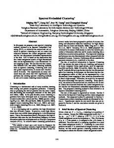
the two-component composite system by the resistor network, a series of runs were generated for constant ␦ / a. As ␦ and a were increased for fixed ␦ / a, the spectral density divided by C共␦ , a兲 = lims→⬁ s2关F共s兲 − F0共s兲兴 or R共␦ , a兲 = limt→⬁ t2 关H共t兲 − H0共t兲兴 was found to approach a limiting form. For fixed ␦ / a, the volume fraction of material between the random rough surface and the y-z (or x-y) plane scales with ␦2 / 共La兲, so that the continuum limit of the spectral density divided by C共␦ , a兲 and R共␦ , a兲 should be a constant. The limiting form of the spectral density normalized by Eq. (44) or Eq. (47) generated from the resistor network results should agree with the continuum limit result when the lengths characterizing the interface roughness are large compared to those of the resistor bonds. As a check on the numerically generated data, the sum rules of Sec. II C were evaluated. The poles at s = 0 共t = 0兲 in F共s兲关H共t兲兴 were obtained from the numerical data by fitting a Lorentzian form in the neighborhood of s = 0 共t = 0兲 to the numerically generated data. Equations (46) and (49) relating the residues at s = 0 or t = 0 to the spectral densities summed over the nonzero si or ti were found to hold to a fraction of a percent, i.e., running the simulation for a fixed value of p1 generated F0 and w␴ satisfying Eqs. (46) and (49) to a fraction of a percent. The limiting forms in Eqs. (44) and (45) for s2关F共s兲 − F0共s兲兴 ⬀ 共1 / V兲兰 d3r兩␪3共rជ兲兩 and Eqs. (47) and (48) for t2关H共t兲 − H0共t兲兴 ⬀ 共1 / V兲兰 d3r兩␪3共rជ兲兩 were also examined. For fixed ␦ / a the constants of proportionality are shown to agree to within a few percent provided that a Ⰶ L. For a 艌 L the statistical correlations along the interface are affected by the finite width of the sample. In this limit the agreement of the constant of proportionality is less satisfactory. In Fig. 1 the spectral density from F共s兲 data is plotted as a function of s = ␴2 / 共␴2 − ␴1兲. The effective conductivity data is obtained for systems with 50% ␴1 and 50% ␴2 for interfaces that average to the y-z plane. The results are labeled by ␦ and a characterizing the statistical properties in Eqs. (6) and (7) of the set of Gaussian random functions. In each figure two curves are presented representing results at fixed ␦ / a for two different sets of 共␦ , a兲. This gives an indication of the convergence of the numerically generated resistor network data to the continuum limit results. Units for ␦ and a are in resistor bond lengths, i.e., ␦ = 1 represents a ␦ of one bond length. In the plots presented, the ratio ␦ / a starts from a high value and decreases through one to a low value. This displays the behavior of the spectral density as one goes from the limit of surfaces that have high peaks falling quickly to narrow valley 共␦ / a Ⰷ 1兲 to the limit of surfaces having smooth tapered hills 共␦ / a Ⰶ 1兲. As expected, the spectral densities generated by the computer simulation are insensitive to the parallel shifting of the mean interface to the right or left of the x-y plane and to the corresponding percentage changes in ␴1 and ␴2 of the system. The rough interfaces generated by the simulation, however, must remain well contained within the finite volume of the resistor network treated by the simulation. In general, for ␦ / a ⬎ 1 the spectral density is a broad flat function of s over the interval 0 艋 s 艋 1. The flat region, which tends to narrow as ␦ / a = 1 is approached, is not featureless. It is composed of three rather low maxima with

relatively large widths. For ␦ / a ⬍ 1 the spectral density continues to narrow reducing to a large peak centered at s = 21 in the extreme ␦ / a Ⰶ 1 limit. In the perturbation theory discussion given in Sec. IV, it will be shown that for ␦ / a → 0 the density of states is a single pole at s = 21 . All of the results presented in Fig. 1 are symmetric about s = 21 . This comes from F共s兲 − F0共s兲 in Eq. (22) and the corresponding expresf f ef f ef f sion for H共t兲 − H0共t兲. Both ␴ef and ␳ef for large 0 −␴ 0 −␳ sized samples (i.e., L → ⬁) are determined by the properties of the systems in the vicinity of their random interfaces. f f ef f ef f and ␳ef should be invariant Consequently, ␴ef 0 −␴ 0 −␳ under the interchange of ␴1 and ␴2. For F共s兲 − F0共s兲 this implies that 1 s

Fs

1

Fs

兺i s −i si i = s 兺i s − 共1i −i si兲 .

共51兲

Similarly, from H共t兲 − H0共t兲 it follows that 1 t

Ht

1

Ht

兺i t −i tii = t 兺i t − 共1i −i ti兲 .

共52兲

Both of these indicate symmetry under reflection through s or t = 21 . The data from the finite network simulations leading to F共s兲 are displayed in Table I. The sum rule F0 − w␴ = p1 = 0.5 of Eq. (46) is evidently satisfied to a few parts per thousand. This provides a nontrivial evaluation of the accuracy of our simulations and of the errors introduced by the finiteness of the network 共L = 128兲 and its discrete nature. The values found for C共␦ , a兲 ⬅ lims→⬁ s2关F共s兲 − F0共s兲兴 of Eq. (44) satisfy the expectation that this quantity is proportional to ␦2 / 共La兲 for ␦ Ⰶ a and to ␦ / L for ␦ Ⰷ a, which followed from Eq. (45) (see Sec. II C). In Fig. 2, corresponding results for the spectral density from H共t兲 of the effective resistivity with an interface which on average gives the x-y plane are presented. The spectral density is plotted as a function of t = ␳2共␳2 − ␳1兲 for the same range of ␦ and a values used to generate the data in Fig. 1. The same general features as found in the results (plotted versus s) in Fig. 1 are found for those (plotted versus t) in Fig. 2. (It should be noted that although the results in Figs. 1 and 2 exhibit general similarities if t = s, in fact t ⫽ s are differently defined variables and the geometries of the two systems in Figs. 1 and 2 are quite different. Even if t were equal to s, the resulting figures are not the same, they are only similar in overall appearance and represent results for differently defined sets of spectral densities.) Once again the results should be symmetric about t = 21 and, in the ␦ / a Ⰶ 1 limit, the perturbation theory discussed in Sec. IV gives a spectral density with a single pole at t = 21 . It is interesting that the results in Figs. 1(e) and 2(e) are very similar in their respective dependences on s and t. This comes from the fact that in this limit the simple poles at s = 1 / 2 or t = 1 / 2 are dominating the respective behaviors of these systems in the weak perturbative limit. The data from the finite network simulations leading to H共t兲 are displayed in Table II. As was the case in Table I, the sum rule H0 − w␳ = p1 = 0.5 of Eq. (49) is usually satisfied to a

144205-7


MCGURN et al.

FIG. 1. A plot of the spectral density of F共s兲 − F0共s兲 divided by C共␦ , a兲 versus s for (a) ␦ / a = 4.00 curves shown for 共␦ , a兲 = 共8 , 2兲 (dashed line) and 共16, 4兲 (solid line); (b) ␦ / a = 1.33 with curves shown for 共␦ , a兲 = 共8 , 6兲 (dashed line) and 共12, 9兲 (solid line); (c) ␦ / a = 1.00 with curves shown for 共␦ , a兲 = 共12, 12兲 (dashed line) and 共16, 16兲 (solid line); (d) ␦ / a = 0.75 with curves shown for 共␦ , a兲 = 共9 , 12兲 (dashed line) and 共12, 16兲 (solid line); and (e) ␦ / a = 0.25 with curves shown for 共␦ , a兲 = 共12, 48兲 (dashed line) and 共16, 64兲 (solid line).

few parts per thousand. Again, this provides a nontrivial evaluation of the accuracy of our simulations and of the errors introduced by the finiteness of the network 共L = 128兲 and its discrete nature. Again, as was the case in Table I, the values found for R共␦ , a兲 ⬅ limt→⬁ t2关H共t兲 − H0共t兲兴 of Eq. (47) satisfy the expectation that this quantity is proportional to ␦2 / 共La兲 for ␦ Ⰶ a and to ␦ / L for ␦ Ⰷ a, which followed from Eq. (48) (see Sec. II C). A consideration for both Figs. 1 and 2 is the effect of the size of the resistor array on the data. At the edges of the

resistor array, the correlations along the random interface will be disrupted. This occurs on the interface within a correlation length of the edges of the array, even with the application of periodic boundary conditions. As a consequence, the effective correlation length of the generated data should be a little less than that for data that would be generated in an infinite system. These correlation length differences will be small (at most of order a / L) in the cases presented in Figs. 1 and 2. The spectral functions in Figs. 1 and 2, however, exhibit only small differences for changes in the correlation

144205-8



TABLE I. Results for F共s兲 from network simulations.

␦

a

−w␴

F0

F0 − w␴

C共␦ , a兲

8 16 8 12 12 16 9 12 12 16

2 4 6 9 12 16 12 16 48 64

0.093 0.180 0.064 0.091 0.080 0.104 0.053 0.069 0.034 0.044

0.406 0.318 0.436 0.408 0.420 0.395 0.446 0.431 0.465 0.453

0.499 0.498 0.500 0.499 0.500 0.499 0.499 0.500 0.499 0.497

0.0326 0.0620 0.0262 0.0376 0.0339 0.0441 0.0233 0.0300 0.0143 0.0177

length that are of the order of magnitude of those discussed above. On pages 10 and 11 of Ref. 38, a discussion of the formal treatment of finite size scaling effects arising in numerical simulations in terms of the dependence of the computed root mean square deviation of a property on the sample size is given. For the spectral densities of the systems treated in Figs. 1 and 2, such a discussion would be extremely computationally intensive and would not lead to new insight into the physics of these systems. It will not be pursued here. Another type of interface that can readily be treated by the simulation technique and is of considerable interest is that of J in periodic interfaces. For this case the operators ⌫ˆ 0 and ⌫ 0 Eqs. (14) and (15) and Eqs. (33) and (34), respectively, exhibit the same periodicity as their buried interfaces. This folJ , ⵜ, lows from the complete translational symmetry of G0, G 0 ⵜ⫻, and the periodicity of the ␪1共rជ兲’s. Consequently, the eigenvalues and eigenvectors of Eqs. (14) and (33) obey Bloch’s theorem: They form bands that are characterized by a Bloch q-vector that lies in the two-dimensional subspace (i.e., plane) of three-dimensional space, which embodies the periodic nature of the interface. These bands have gaps and other typical features, similar to those found in other physical systems that are characterized by spatial periodicity. However, only the q = 0 state from any Bloch band can contribute a nonzero weight Fi or Hi in the spectral expansion of F共s兲 or H共t兲. This statement, which is an exact theorem for continuum composites of infinite volume or periodic boundary conditions,3,4 can be violated to some extent when we deal with finite sized discrete networks. For this reason, we included all the eigenstates whenever we calculated the spectral weight functions g␴共u兲, g␳共v兲. Results of some of those calculations, using interfaces with periodic roughness, are reported below. A detailed treatment of the banding properties of the eigenstates for periodic interfaces will be presented in a future publication.

IV. PERTURBATION THEORY RESULTS

Perturbation theory can be used to obtain the effective conductivity (resistivity) of the buried interface problem as

␦

␦2

2L

2La

0.03125 0.0625 0.03125 0.046 875 0.046 875 0.0625 0.035 156 0.046 875 0.046 875 0.0625

0.125 0.25 0.04167 0.0625 0.046 875 0.0625 0.026 367 2 0.035 156 3 0.011 718 8 0.015 625 0

an expansion in the surface profile function. This is done separately for each of the cases treated in subsections II A and II B. A. Average interface in the y-z plane

For this geometry, start from the current continuity equation ⵜ · Jជ = 0 and write Jជ = −␴共rជ兲ⵜ␾. The scalar function ␾共rជ兲 then satisfies

冋

册

⳵2 ⳵2 + ␾共rជ兲 = 0 ⳵ x2 ⳵ z2

共53兲

on either side of the interface. The boundary conditions for L → ⬁ on ␾共rជ兲 are ␾共z = −L / 2兲 = 0, ␾共z = L / 2兲 = ␾0, and ␾共rជ兲, and the normal component of Jជ 共rជ兲 are continuous at the random interface. The solution for ␾共rជ兲 can be written in the form

冉冊

冉冊

⬁

1 2z 2n␲ ␾L共rជ兲 = ␾0 1 + z e共2n␲/L兲x + 兺 D1共n兲sin 2 L L n=0

冋

⬁

+

兺 D2共n兲cos n=0

册

共2n + 1兲␲ z e关共2n+1兲␲/L兴x , L

for x ⬍ min ␰共z兲, and

冉冊

⬁

共54兲

冉冊

1 2z 2n␲ z e−共2n␲/L兲x ␾ 共rជ兲 = ␾0 1 + + 兺 C1共n兲sin 2 L L n=0 R

⬁

+

冋

兺 C2共n兲cos n=0

册

共2n + 1兲␲ z e−关共2n+1兲␲/L兴x , L

共55兲

for x ⬎ max ␰共z兲. Here account is made of the boundary conditions at z = ± L / 2. In the application of the boundary conditions at the randomly rough interface, the Rayleigh hypothesis33 is assumed to be valid. This assumption is that x ⬍ min ␰共z兲 in Eq. (54) can be replaced by x ⬍ ␰共z兲, and that x ⬎ max ␰共z兲 in Eq. (55) can be replaced by x ⬎ ␰共z兲. The Rayleigh hypothesis is generally found to be valid for Gaussian random systems in which ␦ / a ⬍ 0.1.

144205-9


MCGURN et al.

FIG. 2. A plot of the spectral density of H共t兲 − H0共t兲 divided by R共␦ , a兲 versus t for (a) ␦ / a = 4.00 with curves shown for 共␦ , a兲 = 共8 , 2兲 (dashed line) and 共16, 4兲 (solid line); (b) ␦ / a = 1.33 with curves shown for 共␦ , a兲 = 共8 , 6兲 (dashed line) and 共12, 9兲 (solid line); (c) ␦ / a = 1.00 with curves shown for 共␦ , a兲 = 共12, 12兲 (dashed line) and 共16, 16兲 (solid line); (d) ␦ / a = 0.75 with curves shown for 共␦ , a兲 = 共9 , 12兲 (dashed line) and 共12, 16兲 (solid line); and (e) ␦ / a = 0.25 with curves shown for 共␦ , a兲 = 共12, 48兲 (dashed line) and 共16, 64兲 (solid line).

The first terms on the right-hand sides of Eqs. (54) and (55) are the solutions for ␾L and ␾R in the case of a flat interface. The remaining terms give the change from the flat interface results due to the random disorder in the interface. Consequently, the coefficients D1共n兲, D2共n兲, C1共n兲, and C2共n兲 depend on the surface roughness profile function ␰共z兲 and vanish when ␰共z兲 = 0. In the following, a perturbation expansion is generated by matching the interface boundary conditions in powers of the surface profile function ␰共z兲.

To match the interface boundary conditions, the coefficients C␣共n兲 and D␣共n兲 for ␣ = 1, 2 are written as series in powers of ␰共z兲, so that ⬁

C␣共n兲 = and

144205-10

C␣,i共n兲兺 i=1

共56兲



TABLE II. Results from network simulations for H共t兲.

␦

a

−w␳

H0

H0 − w␳

R共␦ , a兲

8 16 8 12 12 16 9 12 12 16

2 4 6 9 12 16 12 16 48 64

0.086 0.168 0.060 0.087 0.075 0.099 0.050 0.064 0.028 0.035

0.409 0.323 0.439 0.412 0.424 0.400 0.450 0.435 0.470 0.463

0.495 0.491 0.469 0.499 0.499 0.499 0.500 0.499 0.498 0.498

0.0310 0.0606 0.0246 0.0359 0.0323 0.0424 0.0218 0.0284 0.0132 0.0165

␦

␦2

2L

2La

0.03125 0.0625 0.03125 0.046 875 0.046 875 0.0625 0.035 156 0.046 875 0.046 875 0.0625

0.125 0.25 0.04167 0.0625 0.046 875 0.0625 0.026 367 2 0.035 156 3 0.011 718 8 0.015 625 0

⬁

D␣共n兲 =

兺 i=1

D␣,i共n兲.

Here C␣,i共n兲 and D␣,i共n兲 represent all contributions to these coefficients of order i in powers of ␰. Using Eqs. (56) and (57) in Eqs. (54) and (55), a system of equations for D␣,i and C␣,i are determined at the interface. These equations are used below to obtain the solutions for ␾ to first order in ␰共z兲. The continuity of ␾共rជ兲 at x = ␰共z兲 gives 兩␾L共rជ兲兩x=␰共z兲 = 兩 ␾R共rជ兲兩x=␰共z兲. It then follows from Eqs. (54) and (55) that C␣,1共m兲 − D␣,1共m兲 = 0,

冉

冊

冉

冊

d␰ d␰ · ⵜ␾L = ␴2 1,0,− · ⵜ␾R dz dz

␾0 , L

⬁

Jz共1兲

−

冉

冊

冕

Jz共2兲 = − ␴2

␴2 − ␴1 ␾0 共␰m + ␰−m兲, ␴1 + ␴2 L

−

冋

册

共64兲

冋

册

共2n + 1兲共2n + 1兲␲ sin zC2,1共n兲e−关共2n+1兲␲/L兴x , 共65兲 2 L

for x ⬎ ␰共z兲. The average current density for a given surface profile ␰共z兲 is Jz,av =

L/2

dz

冋

1 L

冕

+

1 L2 − ␰共z兲

−L/2

共62兲

共63兲

2n␲ 2␲ ␾0 − ␴2 兺 n cos zC1,1共n兲e−共2n␲/L兲x L L n=0 L

共2n + 1兲␲ d␰共z兲 z , 共61兲 ⫻cos L dz

C1,1共m兲 =

共2n + 1兲␲ d␰共z兲 z . L dz

2n + 1 共2n + 1兲␲ sin zC2,1共n兲e关共2n+1兲␲/L兴x , 2 L

⬁

where ␰共z兲 = 兺 p␰ pei共2p␲z/L兲. Solving Eqs. (58), (60), and (61) gives C1,1共m兲 = D1,1共m兲, C2,1共m兲 = D2,1共m兲,

dz

−L/2

for x ⬍ ␰共z兲, and

共59兲

共60兲

冊

L/2

2n␲ 2␲ ␾0 zC1,1共n兲e共2n␲/L兲x = − ␴1 − ␴1 兺 n cos L L n=0 L

and

␴1 − ␴2 2 ␾0 ␴2C2,1共m兲 + ␴1D2,1共m兲 = ␴1 + ␴2 共2n + 1兲␲ L

冉

冕

The z component of current density is then

for x = ␰共z兲. From this and Eqs. (54) and (55) it follows that

␴2C1,1共m兲 + ␴1D1,1共m兲 = ␴2 − ␴1共␰−m + ␰m兲

␴1 − ␴2 2 ␾0 ␴1 + ␴2 共2n + 1兲␲ L ⫻cos

共58兲

where ␣ = 1 or 2. The continuity of the normal component of the current density at the random interface gives

␴1 1,0,−

C2,1共m兲 =

共57兲

L/2

−L/2

1 L1 + ␰共z兲

冕

L2

␰共z兲

冕

␰共z兲

Jz共1兲dx

−L1

册

Jz共2兲dx dz,

共66兲

where L1 and L2 → ⬁ are the lengths of the ␴1 and ␴2 materials in the x directions. Averaging Eq. (66) over ␰共z兲 gives the average current density 具Jជ 典. The average current density 具Jជ 典 is computed from Eqs. (62)–(66) using 具 ␰ m␰ n典 =

and 144205-11

冑␲a␦2 L

exp −

冉冊 ␲ma L

2

␦n+m,0 ,

共67兲


MCGURN et al.

具共␰n + ␰−n兲2典 =

冑␲a␦2 L

exp −

冉冊 ␲na L

2

⬁

⬁

2␲n 2␲n z+ z, ␰共z兲 = ␰n cos ␾n sin a a n=0 n=1

兺

共2 + ␦−2n,0 + ␦2n,0兲,

兺

共68兲 and ⬁

兺 f共2n + 1兲 ⬇

n=0

冕

F共s兲 − F0共s兲 = ⬁

共69兲

dnf共2n + 1兲.

L 1␴ 1 + L 2␴ 2 ␾ 0 L1 + L2 L

冉冊

4 共␴2 − ␴1兲2 ␾0 冑␲␲a␦2 ␲na + n exp − 2 L L1 + L2 ␴1 + ␴2 L L n=0 ⬁

兺

冊册

. 共74兲

2

.

B. Average interface in the x-y plane

For this geometry, the same formulation as that given in the first paragraph of Sec. IV A is used. The difference here, however, is that the average interface is in the x-y plane, not the y-z plane. As the interface between the two components of the composite is not bounded in the x-y plane, the solution of Eq. (53) for ␾共rជ兲 can now be written in the form

共70兲 [Note: The general form of 具Jz典 in Eq. (70) for the case L1 = L2 can be checked using a rough argument, originally given by Landau and Lifshitz for a bulk disordered medium. This is presented in the Appendix.] For equal concentrations of ␴1 and ␴2, in the L → ⬁ limit for L1 = L2 = L / 2, 1 1 1 ␦␦ F共s兲 − F0共s兲 = 冑␲ s s − 21 L a .

1 1 1 P 2␲ s s − 21

冕

dz

␾⬎共rជ兲 = A⬎ + B⬎z +

1 d 具␰共z兲␰共0兲典. 共72兲 z dz

Here the principal part −共1 / ␲兲P 兰 dz共1 / z兲共d / dz兲具␰共z兲␰共0兲典 = 兰共dk / 2␲兲兩k兩g共k兲, where in the L → ⬁ limit 具␰共z兲␰共0兲典 = 兰共dk / 2␲兲g共k兲eikz. Equations (54)–(66) and (69) can also be used to determine F共s兲 − F0共s兲 for interfaces that are nonrandom and periodic. For a periodic profile function of the form

冕

dk ikx ⬎ e 关C 共k兲e−kz + D⬎共k兲ekz兴, 2␲ 共75兲

where z ⬎ ␰共x兲, and

␾⬍共rជ兲 = A⬍ + B⬍z +

共71兲

Here we use the definition of F共s兲 and F0共s兲 in Eqs. (20)–(24). The above expression has two simple poles at s = 0 and s = 1 / 2. We note that the singularities at these two values of s are generic features of the function F共s兲 that appear for quite arbitrary microstructures: The pole at s = 0 is a result of the fact that the subvolume of the ␴1 constituent percolates in the microstructure of Sec. II A, i.e., a continuous path through that constituent exists between the top and bottom equipotential plates.6 The pole at s = 1 / 2 is a result of the following mathematical property: Although the details of the pole spectrum of F共s兲 (i.e., positions and residues) depend on the precise microstructure, that spectrum usually has an accumulation point at s = 1 / 2, even if all the interfaces are smooth and regular and have no singular points.5 Thus, in general, F共s兲 will have an essential singularity at that point. The simple pole which we found at s = 1 / 2, using perturbation theory, is the remnant of that essential singularity. In the L → ⬁ limit for L1 = L2 = L / 2, Eqs. (54)–(66) and (69) can be used to obtain F共s兲 − F0共s兲 for a general surface profile correlator 具␰共z兲␰共0兲典. We find that F共s兲 − F0共s兲 = −

冉

0

Equation (69) has been used for functions f共2n + 1兲 which depend on C2共n兲. We find 具Jz典 = −

冋

⬁

␰2n ␾2n ␰20 ␲1 1 + 2 兺 + 2 s s − 21 La n=1 La La

共73兲

冕

dk ikx ⬍ e 关C 共k兲e−kz + D⬍共k兲ekz兴, 2␲ 共76兲

where z ⬍ ␰共x兲. From the condition that ␾共z = −L / 2兲 = 0, it follows that L A⬍ = B⬍ 2

共77兲

D⬍共k兲 = − C⬍共k兲ekL .

共78兲

and

Here again the Rayleigh hypothesis,33 i.e., the representation of the solutions for z ⬎ ␰共x兲 by the form valid for z ⬎ max ␰共x兲 and the solutions for z ⬍ ␰共x兲 by the form valid for z ⬍ min ␰共x兲 is assumed. From the condition that ␾共z = L / 2兲 = ␾0, it follows that L ␾0 = A⬎ + B⬎ 2

共79兲

D⬎共k兲 = − C⬎共k兲e−kL .

共80兲

and

Equations (77)–(80) are used to eliminate B⬎, B⬍, D⬎共k兲, and D⬍共k兲 from Eqs. (75) and (76), so that 2 ␾⬎共rជ兲 = A⬎ + 共␾0 − A⬎兲z + L

冕

dk ikx ⬎ e C 共k兲关e−kz − e−kLekz兴 2␲ 共81兲

and

144205-12



冉冊冕

2 ␾⬍共rជ兲 = A⬍ 1 + z + L

dk ikx ⬍ e C 共k兲关e−kz − ekLekz兴. 2␲

具Jz典 = −

共82兲 The coefficients A⬍, A⬎, C⬎共k兲, and C⬍共k兲 are determined as functions of ␰共x兲 by matching boundary conditions at the random interface. The continuity of ␾共rជ兲 and the component of Jជ 共rជ兲 normal to the interface at z = ␰共x兲 gives

␾⬎关z = ␰共x兲兴 = ␾⬍关z = ␰共x兲兴 and

冋

␴2 −

册

冋

共83兲

⫻

册

Expanding in powers of ␰共x兲, we write ⬁

共85兲

n=0

where i = ⬎ or ⬍, and Cin共k兲 represents terms of order n in ␰. Substituting Eqs. (81) and (82) into Eqs. (83) and (84) and using Eq. (85) gives C⬎ 0 共k兲 = 0, C⬎ 1 共k兲 =

C⬎ 2 共k兲

共86兲

␴ 1共 ␴ 2 − ␴ 1兲 1 2 ␾ 0 ˆ ␰共k兲, 共␴2 + ␴1兲2 1 − e−kL L

共87兲

冋

2␾0 ␴ 1共 ␴ 2 − ␴ 1兲 1 = 共␴1 − ␴2兲共ekL + 1兲 3 kL −kL L 共 ␴ 2 + ␴ 1兲 e − e ⫻ ⫻

冕冕

H共t兲 − H0共t兲 = 2冑␲

册

␴2 ␾0 . ␴2 + ␴1

2

L

a L 共90兲

.

2

a L

冉冊

dr e2r + 1 r 2a 2 exp − 2 . r 2r 2␲ e − 1 L

In the L → ⬁ limit H共t兲 − H0共t兲 =

1 1 1 ␦␦ 冑␲ t t − 21 L a .

共92兲

This has the same functional form as that of F共s兲 − F0共s兲 in Eq. (71). Like Eq. (71), this expansion also has two simple poles at t = 0 and t = 1 / 2. These are generic features of the function H共t兲: The pole at t = 0 expresses the fact that the subvolume of the ␴2 constituent does not percolate between the top and bottom plates of the structure of Sec. II B.6 In general, the point t = 1 / 2 is an accumulation point of the pole spectrum of H共t兲, and thus this function usually has an essential singularity at that point.5 The simple pole that we obtained using perturbation theory is, again, the remnant of that essential singularity. In addition, for a general surface profile correlator 具␰共x兲␰共0兲典, 1 1 1 P 2␲ t t − 21

冕

dx

1 d 具␰共x兲␰共0兲典, x dx

which is the same form as Eq. (72) for F共s兲 − F0共s兲. For the nonrandom periodic surface given by ⬁

共89兲

The effective conductivity is determined from the average current 具Jជ 典 = −具␴共rជ兲䉮␾共rជ兲典. Using Eqs. (81), (82), and (85)– (88), the average z component of the current density is found to be

⬁

2␲n 2␲n x+ x, ␰共x兲 = ␰n cos ␾n sin a a n=0 n=1

兺

共88兲

for the first three C⬎ coefficients. Here ␰共x兲 n 共k兲 −ikx ˆ = 兰共dk / 2␲兲e ␰共k兲. In the same way, the C⬍ n 共k兲 coefficients are determined and found to be closely related to the ⬍ ⬎ 兵C⬎ n 共k兲其. The 兵Cn 共k兲其 are obtained from the 兵Cn 共k兲其 by not⬍ ing that −Cn 共k兲 is given from the expression for C⬎ n 共k兲 by replacing L with −L and interchanging ␴1 and ␴2. From Eqs. (83) and (84), the leading order terms in ␰共x兲 give A⬎ = A⬍ =

冉冊冕

1 1 ␦ t t − 21 L

H共t兲 − H0共t兲 = −

dq eqL + 1 ˆ q ␰共k − q兲␰ˆ 共q兲 + 2␴2共ekL − 1兲 2␲ eqL − 1 dq ˆ q␰共k − q兲␰ˆ 共q兲 , 2␲

冉冊冎

dr e + 1 r 2a 2 exp − 2 r 2r 2␲ e − 1 L

␦

In the ␦ = 0 limit this correctly reduces to the effective conductivity of the flat surface system. Using the relationship ␳ef f = 1 / ␴ef f , the difference H共t兲 − H0共t兲, defined in Eqs. (40) and (43), to leading order in ␦ is

共84兲

兺 Cin共k兲,

冕

2r

册冉冊 2

共91兲

d␰共x兲 d␰共x兲 ,0,1 · ⵜ␾⬎共rជ兲 = ␴1 − ,0,1 · ⵜ␾⬍共rជ兲. dx dx

Ci共k兲 =

再冋

共 ␴ 2 − ␴ 1兲 ␴ 2␴ 1 2 ␾ 0 1 + 8冑␲ ␴2 + ␴1 L 共 ␴ 2 + ␴ 1兲

we get

兺

冋

⬁

冉

␰2n ␾2n ␰20 ␲1 1 H共t兲 − H0共t兲 = +兺 + 1 2 2 t t− 2 La n=1 La La

共93兲

冊册

. 共94兲

C. Perturbation theory results

In the limit that ␦ Ⰶ a Ⰶ L, the perturbation theory for F共s兲 − F0共s兲 and H共t兲 − H0共t兲 is very similar. The functional form of F共s兲 − F0共s兲关H共t兲 − H0共t兲兴 exhibits simple poles at s = 0共t = 0兲 and s = 21 共t = 21 兲. These two poles are observed in the ␦ Ⰶ a limit of the s ⬎ 0共t ⬎ 0兲 data plotted in Fig. 1 (Fig. 2). Actually, at s = 1 / 2 or t = 1 / 2 there should be an essential singularity, as explained above.5 An interesting feature of the perturbation theory results is that both F共s兲 − F0共s兲 and H共t兲 − H0共t兲 are proportional to

144205-13


MCGURN et al.

FIG. 3. Plot of the weight defined as lims→⬁ s2关F共s兲 − F0共s兲兴 / 共␦2 / La兲 or limt→⬁ t2关H共t兲 − H0共t兲兴 / 共␦2 / La兲 versus ratio = ␦ / a for (a) the Gaussian randomly rough interface and (b) the periodic cosine interface.

␦2 / 共La兲. This suggests a scaling relation for F共s兲 − F0共s兲,

H共t兲 − H0共t兲, and their sum rules. To see if this is the case, we have considered plots of the sum rules of F共s兲 − F0共s兲 and H共t兲 − H0共t兲 displaying such scaling. In Fig. 3(a) plots of the sum rules in Eqs. (44) and (47) for Gaussian randomly rough interfaces are presented for various ␦ and a. The results are plotted so that the vertical scale shows lims→⬁ s2关F共s兲 − F0共s兲兴 / 共␦2 / La兲 or limt→⬁ t2关H共t兲 − H0共t兲兴 / 共␦2 / La兲 and the horizontal scale shows ␦ / a. The horizontal line indicates the perturbation theory limit and the dashed line is a Pade fit to the data. The Pade form used is y = 关1 – 0.8260共␦ / a兲兴 / 关冑␲ + 0.9179共␦ / a兲兴, where y is on the vertical axis. This form forces the Pade form to a fit to the perturbation theory result 共1 / 冑␲兲 in the ␦ / a = 0 limit. The numerically generated data lies on a universal curve given by the Pade form when plotted as described above. At small ␦ / a the numerically generated points closest to the Pade results are the ones with larger ␦ and a. This suggests that the discrepancy between the numerically generated data and the Pade form is mainly due to the discrete nature of the resistor network. [By this we mean that in modeling a continuum system by a discrete finite sized lattice, not all length scales are treated correctly (see a discussion of aliasing in Ref. 39). The numerical simulation of the lattice model does not accu-

rately treat lengths less than the lattice constant and lengths greater than the lattice size. The continuum solutions, however, contain all length scales, although with varying degrees of importance. The limit ␦ / a → 0 is represented in the lattice by ␦ / a=(lattice constant)/(length of a side of the total lattice). This may differ form the ␦ / a → 0 limit of the continuum model.] The general decrease of the Pade form results in Fig. 3(a) with increasing ␦ / a is consistent with the discussions given below Eq. (45) for the dependence of p3 on ␦, a, and L. We remind the reader, however, that our computer data are limited by the discrete nature and finite size of the lattice. In Fig. 3(b) a similar plot to that in Fig. 3(a) is given, but for periodic interfaces.40 For these results the interfaces are given by ␰共z兲 = ␦ cos共2␲ / a兲z for the geometry of Sec. II A or by ␰共x兲 = ␦ cos共2␲ / a兲x for the geometry of Sec. II B. The data in Fig. 3(b) are scaled in the same manner as that in Fig. 3(a). The horizontal line gives the perturbation-limiting form, and the dashed line is a Pade fit with y = 关1.571– 0.137共␦ / a兲兴 / 关1 + 2.414共␦ / a兲兴 where y is the vertical axis, and y at ␦ / a = 0 is fixed on the value ␲ / 2 obtained from perturbation theory. The data fall on a universal curve given by the Pade form, and the discrepancies between the numerically generated data and the Pade form again seem to come from the effects of a discrete lattice. Again a decrease in the Pade form is observed with increasing ␦ / a, and this is consistent with out discussions of the dependence of p3 on ␦, a, and L. An additional condition that ␴ef f and ␳ef f must satisfy is the reciprocity relation.10 This is a relation between ␴ef f and ␳ef f defined on dual lattices. A good discussion of this relation can be found in Sec. 3.2 of Ref. 18. Since the square lattice is self-dual, the reciprocity relation relates the perturbation theory results for F共s兲 and H共t兲, so that ␴ef f 共␴1 , ␴2 , p1兲 / ␴2 = ␴1 / ␴ef f 共␴2 , ␴1 , p1兲 = ␳ef f 共␴2 , ␴1 , p1兲 / ␳1. This relation is satisfied by the perturbation results in Eqs. (71) and (92) since interchanging ␴1 and ␴2 in t = ␳2 / 共␳2 − ␳1兲 gives t⬘ = ␳1 / 共␳1 − ␳2兲 = ␴2 / 共␴2 − ␴1兲 = s. As the perturbation theory gives expressions for F共s兲 and H共t兲 that map into one another under interchanging s and t, the reciprocity relation is satisfied.

V. SURFACE PLASMONS AT A RANDOMLY ROUGH INTERFACE

In this section the long wavelength dispersion relation of surface plasmons on a one-dimensionally randomly rough dielectric interface is related to the functions F共s兲 − F0共s兲 and H共t兲 − H0共t兲. Two cases of surface plasmon propagation along the rough interface are treated: (a) propagation parallel to the grooves of the one-dimensional roughness and (b) propagation perpendicular to the grooves of the one-dimensional roughness. Applications of the relationship are given. The propagation of surface plasmons along the random interfaces is considered for the geometries given in Secs. II A and II B. For the surface plasmon considerations, however, the material with conductivity ␴1 in Secs. II A and II B is replaced by a material with dielectric constant ⑀共␻兲 and

144205-14



the material with conductivity ␴2 is replaced by vacuum. Results for the resistor network can be used in the treatment of these two dielectric geometries, as in the continuum limit the conductivity problems studied in Secs. II and IV are isomorphic to the dielectric media problems. Replacing ␴1 by ⑀1, ␴2 by ⑀2, and ␴ef f by ⑀ef f maps the two different problems onto one another so that results for one can be used to describe the other. A. Dispersion relation: propagation parallel to the grooves

To relate H共t兲 − H0共t兲 to the surface plasmon dispersion relation for propagation parallel to the grooves of the onedimensionally rough interface, consider the parallel plate geometry of Sec. II B. The region above the random interface is vacuum and the region below the interface is filled with an homogeneous isotropic dielectric characterized by ⑀共␻兲. The potential difference between the plates in the following considerations is not fixed, but the system operates as a capacitor containing a quasistatic electric field. The surface plasmon modes treated in this geometry propagate in the y direction. The upper plate has a quasistatic surface charge density, qs共x , y , ␻兲 of frequency ␻, and the lower plate has a surface charge density −qs共x , y , ␻兲. The spatial variations of qs共x , y , ␻兲 are considered to be on length scales much larger than those characterizing the roughness of the randomly rough interface (i.e., ␦, a). Consequently, the response of the system to qs共x , y , ␻兲 is determined by the effective dielectric properties of the random media, so that ⌬V共x,y, ␻兲 = 4␲L

f ⑀ef 0

共96兲

,

where the subscripts 0 indicate flat interface quantities. Here the charge densities qs共x , y , ␻兲 driving the systems in Eqs. (95) and (96) are the same. From Eqs. (95) and (96) it then follows that ⌬V共x,y, ␻兲 − ⌬V0共x,y, ␻兲 = 4␲L

冉

冋

冊

1 1 ef f − ef f qs共x,y, ␻兲. ⑀ ⑀0

⌬V共y, ␻兲 = 4␲qs共y, ␻兲

1 k

␾共y,z, ␻兲 = 共Ae−kz + A1ek共z−L/2兲兲eiky

共98兲

above the interface, and

␾共y,z, ␻兲 = 共Bekz + B1e−k共z+L/2兲兲eiky

共99兲

below the interface. Matching the boundary conditions at the interface and the surface charge density [i.e., ±qs共y , ␻兲] boundary conditions at the upper and lower plates deter-

再冋

册冉

1 1 1 + 1 + kL ef f − ef f ⑀共␻兲 ⑀ ⑀0

冊冎

.

共101兲

The condition for a surface plasmon mode to exist is that ⌬V共y , ␻兲 = 0 for nonzero qs共y , ␻兲. This gives 0= =

冉

1 1 1 + 1 + kL ef f − ef f ⑀共␻兲 ⑀ ⑀0

冊

1 + 1 − kL关H共t兲 − H0共t兲兴, ⑀共␻兲

共102兲

where t = ⑀共␻兲 / 关⑀共␻兲 − 1兴 as the equation determining the surface plasmon dispersion relation on the random interface in the L → ⬁ limit. In the perturbation theory limit discussed in Sec. IV B, we find from Eqs. (92) and (102) that 2 关⑀共␻兲 − 1兴2 ␦2 冑␲ 关⑀共␻兲 + 1兴2 a k

共103兲

determines the surface plasmon dispersion relation at long wavelengths. The dispersion relation on the weakly random rough surface of Sec. IV B can also be computed from results of a Green’s function scattering theory developed in Refs. 41 and 42. It is found that the dispersion relation from Refs. 41 and 42 is determined by 0=1−

2共1 + cos2␪兲关⑀共␻兲 − 1兴2 ␦2 k. 冑␲ 关⑀共␻兲 + 1兴2 a

共104兲

Here ␪ is the angle between the surface plasmon wave vector in the plane of the mean surface and the direction perpendicular to the grooves of the one-dimensionally randomly rough interface. Equations (103) and (104) are in agreement.

共97兲 The flat surface surface-plasmon of quasistatic frequency ␻ propagating in the y direction has an electric potential of the form

册

qs共y, ␻兲 1 + 1 tanh共kL/2兲, 共100兲 k ⑀共␻兲

so that the difference in potential between the plates depends only on y. Substituting Eq. (100) into Eq. (97) for large L gives

共95兲

where ⌬V共x , y , ␻兲 is the potential between the plates at 共x , y兲 and ⑀ef f is the effective dielectric constant. For a flat interface, Eq. (95) becomes qs共x,y, ␻兲

⌬V0共y, ␻兲 = 4␲

0=1−

qs共x,y, ␻兲 , ⑀ef f

⌬V0共x,y, ␻兲 = 4␲L

mines A, A1, B, and B1. (Notice that the charge density for a plasmon propagating in the y direction has no x dependence in the approximation used here.) From these coefficients it is found that

B. Dispersion relation: Propagation perpendicular to the grooves

To relate F共s兲 − F0共s兲 and H共t兲 − H0共t兲 to the surface plasmon dispersion relation for propagation perpendicular to the grooves of the one-dimensionally rough interface, consider the parallel plate geometry of Sec. II A. The plasmon now travels in the z direction. (Note that the discussions in this section are quite separate from those made in Sec. V A. Section V A treated the system described by the geometry in Sec. II B, whereas the discussion in this section is for a system described by the geometry in Sec. II A. These figures represent two distinct and different physical systems.) The

144205-15


MCGURN et al.

region to the left of the random interface is filled with an homogeneous isotropic dielectric characterized by ⑀共␻兲 and the region to the right of the random interface is vacuum. The potential difference between the upper and lower plates is zero. We consider the case in which the wavelength of the surface plasmon is much greater than the parameters a and ␦ characterizing the surface roughness. In this limit the response of the system to fields and charges far from the surface can be described in terms of an effective dielectric constant. The scalar potential of the surface plasmons with quasistatic frequency ␻ is then taken to be of the form

␾共x,z, ␻兲 = f共kz兲␾0共x, ␻兲,

共105兲

Equations (109)–(111) then give (setting L⬘ = L)

⑀共␻兲 + 1 = − ⑀共␻兲

共106兲

in the region to the left of the interface, with

␾0共x, ␻兲 = Be−k共x−L/2兲

0 = 关⑀共␻兲 + 1兴 − kL兵⑀共␻兲关H共t兲 − H0共t兲兴 + F共s兲 − F0共s兲其共113兲 for kL Ⰶ 1. In the perturbation theory limit discussed in Sec. IV, Eq. (113) yields

L⬘Dx共x = L⬘/2,z, ␻兲 . ⑀ef f 共108兲

Here Dx共x = L / 2 , z , ␻兲 is viewed as being proportional to a surface charge density on a fictitious set of capacitor plates at x = L⬘ / 2 and x = −L⬘ / 2. The charge densities on the plates are equal in magnitude and opposite in sign. From Eqs. (105)–(108) it then follows that

冋

A=B 1+

册

kL⬘ . ⑀ef f

共109兲

A second relationship between A and B can be obtained ⬁ dxDz共x , z = −L / 2 , ␻兲 = 0. This is a statement that from 兰−⬁ there is no net charge on the plate at z = −L / 2 and follows from the boundary conditions ␾共x , z = L / 2 , ␻兲 − ␾共x , z = −L / 2 , ␻兲 = 0. From Eqs. (105)–(107) we find that

冕冕 ⬁

0=

dxDz共x,− L/2, ␻兲 = − 关⑀共␻兲A + B兴

−⬁

−

L⬘/2

−L⬘/2

冏冏 df dr

L⬘/2

−L⬘/2

r=−kL/2

dxDz共x,− L/2, ␻兲,

共110兲

dxDz共x,− L/2, ␻兲 ⬇ − k⑀⬘ef f BL⬘

共114兲

as the condition determining the surface plasmon dispersion relation. This agrees with the results in Eq. (104), which was obtained by another method.41,42

冏冏 df dr

C. Effective boundary conditions for one-dimensionally rough interfaces

It is interesting to note that the above results for surface plasmon propagation on a one-dimensionally randomly rough interface, in the limit of long wavelength, can be obtained by representing the effects of the interface roughness by a set of effective boundary conditions defined over the plane of the mean random interface. Consider a random dielectric-vacuum interface described by the surface profile function z = ␰共x兲. Let us replace the rough interface and its boundary conditions by a smooth surface at z = 0 supporting a position-dependent effective surface polarizations.43 This polarization is chosen so as to reproduce the results in Eqs. (102) and (113). To do this, the effective surface polarization is taken to be a vector field with x and z components defined by Ps,x共x兲 = ␹xEx关x, ␰共x兲+兴,

.

In the above, ⑀⬘ is found by replacing ␳ 1 / ⑀共␻兲, and ␳2 by 1 in Eq. (40).

ef f

共116兲

for the corresponding z components of the quantities occurring in Eq. (115). There is no roughness in the y direction, so that the y component of effective surface polarization is zero, i.e., ␹y共x兲 = 0. The susceptibilities for determining the average fields above and below the interface are then written in terms of F共s兲 − F0共s兲 and H共t兲 − H0共t兲 as 4␲␹x = − L关F共s兲 − F0共s兲兴

共117兲

4␲␹z = L关H共t兲 − H0共t兲兴.

共118兲

and

r=−kL/2

by 1 / ⑀⬘ , ␳1 by ef f

共115兲

where Ps,x共x兲 is the x component of polarization per area located at 共x , z = 0兲, ␹x共x兲 is the susceptibility at 共x , z = 0兲, Ex关x , ␰共x兲+兴 is the x component of the electric field in the vacuum above the surface, and by

共111兲 ef f

4 关⑀共␻兲 − 1兴2 ␦2 冑␲ 关⑀共␻兲 + 1兴2 a k

Ps,z共x兲 = ␹zEz关x, ␰共x兲+兴

and for kL⬘ Ⰶ 1 from 具Dz共x , −L / 2 , ␻兲典 = ⑀⬘ef f 具Ez共x , −L / 2 , ␻兲典 ⬇ −⑀⬘ef f kB共df / dr兲兩r=−kL/2 that

冕

0=1−

共107兲

in the region to the right of the interface. From the discussion given in Sec. V A for plasmons moving in a system with the geometry of Sec. II B, it is expected from Eq. (95) that for L⬘ Ⰷ ␦, a,

␾共x = L⬘/2,z, ␻兲 − ␾共x = − L⬘/2,z, ␻兲 = −

共112兲

as the condition for a plasmon to exist on the rough interface. In terms of H共t兲 − H0共t兲 for t = ⑀共␻兲 / 关⑀共␻兲 − 1兴 and F共s兲 − F0共s兲 for s = 1 / 关1 − ⑀共␻兲兴 Eq. (112) becomes

where f共kz兲 = sin kz for kL / 2 = n␲ or f共kz兲 = cos kz for kL / 2 = 共2n + 1兲␲ / 2 with n = 0 , 1 , 2 , . . . and

␾0共x, ␻兲 = Aek共x+L/2兲

kL − kL⑀ef f ⑀⬘ef f

Here t = ⑀共␻兲 / 共⑀共␻兲 − 1兲, s = 1 / 关1 − ⑀共␻兲兴, ⑀共␻兲 is the dielectric constant of the medium below the random interface, and

144205-16



L → ⬁ is the separation of the two parallel plates used in the determination of F共s兲 − F0共s兲 and H共t兲 − H0共t兲. The boundary conditions at the z = ␰共x兲 interface are replaced by effective boundary conditions on the z = 0 plane which are written in terms of the effective surface polarizations defined in Eqs. (115)–(118). The new boundary condiជ = 0 given by tions at z = 0 are from ⵜ ⫻ E 0 = E+x 共x兲 − E−x 共x兲 + 4␲

⳵ Ps,z共x兲 , ⳵x

共119兲

of F共s兲 − F0共s兲 and H共t兲 − H0共t兲 for electron motions parallel and perpendicular to the grooves of the one-dimensionally rough interface. Given these expressions, Eqs. (6) and (7) of Ref. 44 can be used to compute the probability per unit path length, per unit energy, of the electron scattering with energy loss E = h␻. To compute ␾ind共␳ជ , z ; ␻兲 the effective boundary conditions of Sec. V C are used. The electric quasistatic potential in the presence of the surface roughness is given throughout space by

where E+x 共x兲 and E−x 共x兲 are the average electric fields immeជ diately above and below the z = 0 interface, and from ⵜ · D = 0 given by 0=

Dz+共x兲

−

Dz−共x兲

⳵ Ps,x共x兲 , + 4␲ ⳵x

␾r共␳ជ ,z;t兲 =

共120兲

d2Q ext ជ ជ ␾ 共Q, ␻兲eiQ␳ជ +Qz , 共2␲兲2

冕

d2Q ind ជ ជ ␾ 共Q, ␻兲eiQ␳ជ −Qz , 共2␲兲2

共125兲

␾共z兲 = B1e−Q共z+z0兲 + B2eQ共z+z0兲

共126兲

ជ ,− z ; ␻兲 = ␾ext共Q 0

− 2␲e Q

共128兲

and

ជ ,− z ; ␻兲 = B , ␾ind共Q 0 2

共129兲

where B2 =

2␲e ⑀共␻兲 − 1 + 4␲Q关⑀共␻兲␹z + Q2x ␹x/Q2兴 −2Qz 0, e Q ⑀共␻兲 + 1 + 4␲Q关− ⑀共␻兲␹z + Q2x ␹x/Q2兴共130兲

and

ជ , ␻兲 = − B2 . g共Q B1

共131兲

In the limit ␻ / v → 0 for motion parallel to the grooves,

ជ , ␻兲 e2Qz0g共Q =

共123兲

is the induced electric potential in the z = −z0 plane due to the interaction of the electron with the dielectric medium above the interface. In the following, the surface response function for a rough interface, g共Q , −z0 , ␻兲, will be expressed in terms

共127兲

for z ⬍ −z0. The boundary conditions for the determination of A, B1, B2, and C are (a) at z = −z0, ⳵␾+ / ⳵z − ⳵␾− / ⳵z = 4␲e, ␾+ = ␾−, (b) at z = 0 Eqs. (119) and (120), and (c) at z → ± ⬁ the fields are zero. Solving the boundary value problem gives

共122兲

where ␳ជ = 共x , y兲 is a two-dimensional vector parallel to the ជ , −z , ␻兲, which in positioninterface. The potential ␾ind共Q 0 frequency space is given by

␾ind共␳ជ ,z; ␻兲 =

共124兲

for 0 ⬎ z ⬎ −z0 (here the B2 term is the induced potential seen by the electron), and

共121兲

ជ , −z , ␻兲 is the spectral component of the electric Here ␾ext共Q 0 potential from the electron in the case that no dielectric medium is present, and in position-frequency space we have

冕

, ␻=Qyv

␾共z兲 = Ae−Qz

␾共z兲 = CeQ共z+z0兲

Recently Mendoza et al.44 (see also Refs. 45–47) have developed a theory for determining the small energy losses of electrons with energies of order of 100 KeV moving parallel to a dielectric surface. The mean dielectric surface is taken at the z = 0 plane with the dielectric in the region above the plane and vacuum below the plane, and the electron moves with position coordinates 共x = 0 , y = vt , z = −z0兲. (Note: This is slightly different from the other treatments given in this paper which have taken the dielectric to be below the surface. To facilitate the discussions here, we shall use the geometry and notation in Mendoza et al.44 in this subsection.) The losses arise from the polarization of the dielectric medium, and are related to the surface response function, g共Q , −z0 , ␻兲, defined by

␾ext共␳ជ ,z; ␻兲 =

冏

for z ⬎ 0, and

D. Electron energy loss for motion parallel to a surface

ជ ,− z , ␻兲 = − g共Q,− z , ␻兲␾ext共Q ជ ,z , ␻兲. ␾ 共Q 0 0 0

d2Q iQជ ·␳ជ e ␾共z兲e−i␻t 共2␲兲2

where

where Dz+共x兲 and Dz−共x兲 are the average displacement fields immediately above and below the z = 0 interface respectively. Using these conditions to compute the dispersion relations of the surface plasmons reproduces the results in Sec. V A and V B.

ind

冕冏

⑀共␻兲 − 1 + LQ兵⑀共␻兲关H共t兲 − H0共t兲兴 − F共s兲 + F0共s兲其 , ⑀共␻兲 + 1 − LQ兵⑀共␻兲关H共t兲 − H0共t兲兴 + F共s兲 − F0共s兲其共132兲

where t = ⑀共␻兲 / 关⑀共␻兲 − 1兴 and s = 1 / 关1 − ⑀共␻兲兴. In the same limit for motion perpendicular to the grooves, a solution similar to that outlined above gives

144205-17


MCGURN et al.

ជ , ␻兲 = ⑀共␻兲 − 1 + LQ⑀共␻兲关H共t兲 − H0共t兲兴 . e2Qz0g共Q ⑀共␻兲 + 1 − LQ⑀共␻兲关H共t兲 − H0共t兲兴

G共p␻兲 = 1/兵关G0共p␻兲兴−1 − M共p兲其. 共133兲

E. Reflection of p-polarized electromagnetic waves from a one-dimensionally randomly rough surface near normal incidence

It has been important to us in our discussions of F共s兲 − F0共s兲 and H共t兲 − H0共t兲 to show that these functions are not just mathematical curiosities, but that they are related to a number of physically measurable and important properties of surfaces. In this section, the functions F共s兲 − F0共s兲 and H共t兲 − H0共t兲 are also related to the reflectivity of p-polarized light near normal incidence from one-dimensionally randomly rough interfaces. This is a very basic optical property of rough surfaces. In these considerations, we treat electromagnetic waves of quasistatic frequency ␻ incident from vacuum onto a dielectric medium that is uniform, isotropic, and characterized by a dielectric constant ⑀共␻兲. The plane of incidence is taken to be either parallel or perpendicular to the grooves of the onedimensionally random interface. We assume that the wavelength ␭ Ⰷ ␦ , a and only calculate the specular reflection, but not diffuse scattering. 1. Plane of incidence perpendicular to the grooves of the onedimensional surface

In the considerations given here the x-y plane is the mean plane of the vacuum-dielectric interface. On a flat vacuum-dielectric interface, the Fresnel coefficient for the reflection of p-polarized light is41,42 R0共p兲 =

⑀共␻兲␣0共p␻兲 − ␣共p␻兲 . ⑀共␻兲␣0共p␻兲 + ␣共p␻兲

共134兲

Here p is the component of the wave vector of the incident planewave of electromagnetic radiation in the x-y plane, ␣0共p␻兲 = 关␻2 / c2 − p2兴1/2, and ␣共p␻兲 = 关⑀␻2 / c2 − p2兴1/2 with Re ␣共p␻兲, Im ␣共p␻兲 ⬎ 0. For the rough interface scattering geometry of this section, Eqs. (8), (13b), and (17) of Ref. 42 give an average Fresnel coefficient of the form

⑀共␻兲␣0共p␻兲 − ␣共p␻兲 + i⑀共␻兲M共p兲 . Rr共p兲 = ⑀共␻兲␣0共p␻兲 + ␣共p␻兲 − i⑀共␻兲M共p兲

共135兲

Here the average Fresnel coefficient of the rough interface is defined from Eq. (8) of Ref. 42 by 具R共p 兩 k兲典 = 2␲␦共p − k兲Rr共p兲 and M共p兲 (Given in the pole approximation in Eq. (17) of Ref. 42.) is the self-energy correction of the average single particle Green’s function for surface plasmon propagation on the rough interface. (The Green’s function is averaged over the random roughness of the interface.) The average Greens function for the propagation of a surface plasmon of wavevector p and frequency ␻ on the random interface, G共p␻兲, is given in terms of M共p兲 by

共136兲

Here G0共p␻兲 = i⑀共␻兲 / 关⑀共␻兲␣0共p␻兲 + ␣共p␻兲兴 is the surface plasmon Green’s function for propagation on a flat surface. Using M共k兲 from Eqs. (18) and (19) of Ref. 42 and Eq. (135) evaluated at normal incidence gives

⑀共␻兲 − ⑀共␻兲1/2 + i⑀共␻兲共␻/c兲M 0 , ⑀共␻兲 + ⑀共␻兲1/2 − i⑀共␻兲共␻/c兲M 0

Rr共p = 0兲 =

共137兲

where M0 = −

F共s兲 − F0共s兲 1 关⑀共␻兲 − 1兴2 ␴2 =−L . 2 冑␲ ⑀共␻兲 ⑀共␻兲 + 1 a ⑀共␻兲2 2

共138兲 The correction M 0 due to surface roughness scattering is seen to be divergent at ⑀共␻兲 = 0 and ⑀ = −1. These singularities are prominent in determining the effects of surface roughness on the reflectance at normal incidence. The results in Eqs. (137) and (138) agree in the limit that ⑀ → −1 with the reflectivity results to leading order in the surface roughness calculated using the boundary conditions in Sec. V C. 2. Plane of incidence parallel to the grooves of the onedimensional surface

To obtain the Fresnel coefficient for light incident in an arbitrary plane of incidence perpendicular to the onedimensionally rough interface, Eq. (135) and results in Ref. 41 can be used. Reference 41 contains expressions for the Green’s function describing the propagation of surface plasmons along the interface at an arbitrary angle to the grooves of the one-dimensionally rough interface. These expressions give the self-energy M 0 in the limit of weak roughness. The resulting Fresnel coefficient is obtained from Eq. (137) with M 0 of the form M0 = −

1 关⑀共␻兲 − 1兴2 2 ␴2 冑␲ ⑀共␻兲2 ⑀共␻兲 + 1 sin ␾i a 2

=−L

F共t兲 − F0共t兲 2 sin ␾i . ⑀共␻兲2

共139兲

Here ␾i is the angle between the magnetic field of the incident electromagnetic wave and the direction perpendicular to the grooves of the grating. At ␾i = ␲ / 2 the results in Eqs. (138) and (139) are found to agree, to leading order in the interface roughness, with the reflectivity computed using the boundary conditions of Sec. V C. 3. Evaluation of reflectivity for ion crystals

In this subsection Eqs. (137)–(139) are evaluated for a vacuum-CdS interface at normal incidence of light. Results are presented for magnetic field polarizations parallel and perpendicular to the grooves of a one-dimensionally random rough surface. In these evaluations the dielectric function of CdS is given by the form48

144205-18



FIG. 4. Plot of the reflectance versus frequency 共␻ / ␻t兲 for CdS. Results are shown for the case in which the magnetic field of the incident light is parallel (solid) and perpendicular (dashed) to the grooves of the one-dimensionally rough interface.

⑀共␻兲 = ⑀0

␻2l − ␻2 − i␻c␻ ␻2t − ␻2 − i␻c␻

,

共140兲

where ⑀0 = 5.4, ␻t = 232.0 cm−1, ␻l = 298.0 cm−1, and ␻c = 6.9 cm−1.48 Results are presented in Fig. 4 for the reflectivity versus frequency. The one-dimensionally rough surface is Gaussian random characterized by ␻t␴ = 0.1 and ␻ta = 1.0. For the case in which the magnetic field is parallel to the grooves of the one-dimensionally rough surface a dip in the reflectance at ␻ / ␻t = 1.243 is observed. This arises from the singularity in Eq. (138) at ⑀共␻兲 = −1. Aside from this feature the reflectance is little changed from the unperturbed reflectance. For the case in which the magnetic field is perpendicular to the grooves of the one-dimensionally rough surface ␾i = 0 in Eqs. (139) and the reflectance is given by the unperturbed reflectance.

VI. LAYERED INTERFACES

In certain instances the results presented above for single interfaces should generalize to systems of multiple interfaces that on average are parallel to one another. For interfaces that are at separations far from each other, it is expected that each interface can be separately viewed as interacting with an effective medium which accounts for the average effects of the other interfaces on the system. This should be the case when the average separation between the interfaces is much greater than the parameters characterizing the surface roughness. In this limit a given interface in the system sees only an average effect of the electric field fluctuations created by the presence of its neighboring random interfaces. To facilitate this picture of multiple random interfaces we will develop below an effective circuit representation for single interfaces and then suggest a generalization to multiple interfaces. It is interesting to note from Eq. (24) that if both ␴1 and ␴2 are real and positive, then s ⬍ 0 or s ⬎ 1 and F共s兲 − F0共s兲 ⬎ 0. From Eq. (22) this indicates that the conductance of the system with an average interface in the y-z plane is

decreased by interface roughness. The effective interface ef f ef f f conductance, ␴int , defined by ␴int = ␴ef f − ␴ef 0 , is seen to be ef f negative, and for weakly rough surfaces 兩␴int 兩 is small. A useful way of viewing the system in terms of an equivalent electrical circuit is to think of the layer of conductance ␴1, the layer of conductance ␴2, and the interface with interface ef f as a set of three parallel resistors across conductance ␴int ef f 兩 (i.e., which a constant potential is applied. For small 兩␴int large interface resistances) the resistance of the system is ef f 兩 bedominated by the layers of ␴1 and ␴2. Only when 兩␴int comes large does it significantly affect the properties of the system. A drawback of this equivalent circuit representation is that the effective interface resistance is negative. It is expected that the equivalent circuit representation is easily generalizable to a system of multiple interfaces that are on mean parallel to the y-z plane and that in this case the multiple interfaces at sufficient interface separations add like parallel resistors. An explanation of the decrease in the effective conductivity of the system with a rough interface from the smooth surface case comes from an examination of the region along the x axis that bounds the random interface [see Fig. 5(a)]. For the smooth interface, this region consists of a layer of high conductivity and a layer of low conductivity. The current flow is set by the layer of high conductivity. For the random interface all linear paths between the plates at z = L / 2 and z = −L / 2 intersect materials of both high and low conductivity. This reduces the net conductivity in this region. For H共t兲 − H0共t兲 we note from Eq. (43) that if both ␳1 and ␳2 are real and positive, then H共t兲 − H0共t兲 ⬎ 0 for t ⬍ 0 and t ⬎ 0. The resistance of two slabs connected in series is, consequently, always decreased by interface roughness, and from Eqs. (40) and (41) the effective interface resistivity ef f f ␳int = ␳ef f − ␳ef 0 is found to be negative. An equivalent circuit representation for this slab geometry is that of three resistors in series. These represent the layer of resistivity ␳1, the layer of resistivity ␳2, and the resistivity of the interface layer. A drawback in this equivalent circuit representation is that the effective resistivity of the interface layer is negative, but the equivalent series resistor representation should be directly generalizable to a system of multiple interfaces that are on mean parallel to the x-y plane and at sufficient interface separations form one another. In these systems the effective resistivity is decreased from the smooth surface results due to surface roughness. This arises due to the tongues of low resistivity media that protrude into the regions which would otherwise, in the smooth surface system, contain high resistivity material [see Fig. 5(b)]. These tongues provide low resistivity paths that lower the effective resistivity of the system with a random interface. The limiting factor on the equivalent circuit representation is the effects of surface roughness fluctuations at one surface on the potential seen at another surface. An estimate of the importance of fluctuations in the interface roughness on the interaction between interfaces can be made by considering the potential at the mean surface of an interface due to a small localized fluctuation on a neighboring interface. We consider how a cylindrical fluctuation that maintains the average surface field and profile on one interface affects the

144205-19


MCGURN et al.

polar coordinates with ␪ measured relative to kˆ. This potential form generalizes in the limit of far fields for a cylinder of arbitrary bounded cross sectional shape of area S. Next consider two adjacent interfaces in a layered medium. The potential difference between the two inner interfaces in the geometry of Fig. 5(c) is ⌬␾ ⬀ d2E, where E is the average field at the mean interface. A fluctuation on the lower interface can be modeled as a set of two cylinder dipoles of crosssectional areas ␦a (here ␦ and a define the Gaussian random surface profile statistics) that are oppositely directed along the kˆ direction. One dipole cylinder is located at 共x = −a / 2 , z = ␦ / 2兲 relative to a coordinate system whose origin lies on the mean surface of the lower interface and the other is located at 共x = a / 2 , z = −␦ / 2兲. The intensity of the dipole moment on each of the two cylinders is taken to be proportional to ␦aE. The electrostatic potential on the upper interface at a point adjacent to the a surface fluctuation on the lower interface is then approximately ⌬␾dipole ⬀ ␦2aE / d22. The ratio ⌬␾dipole / ⌬␾ ⬀ ␦2a / d32 must be small for the interfaces to be treated in an equivalent resistor scheme that ignores the detailed effects of surface fluctuations on adjacent interfaces. A similar argument can be applied to the geometry in Fig. 5(d). Here two dipoles oppositely directed along the kˆ direction are located at 共x = ␦ / 2 , z = a / 2兲 and 共x = −␦ / 2 , z = −a / 2兲 relative to a coordinate system whose origin lies on the mean surface of the left hand interface. On the right-hand interface, separated by a distance d2 form the left-hand interface, the potential adjacent to this fluctuation is ⌬␾dipole ⬀ ␦a2E / d22. The change in electrostatic potential observed in moving a distance comparable to d2 in the kˆ direction is ⌬␾ ⬀ d2E. For the effects of the fluctuations to be small, again ⌬␾dipole / ⌬␾ = ␦a2 / d23 must be small. Another way of arriving at an estimate of the effects of surface fluctuations on the interaction between adjacent interfaces is to treat the surface roughness on an interface as a position dependent dipole distribution on the mean plane of the interface. The total dipole moment averages to zero over the interface. For the case in Fig. 5(c), let the lower of the two embedded interfaces have a dipole density given by p共x兲 with Gaussian random statistics, i.e., 具p共x兲典 = 0 and 具p共x兲p共x⬘兲典 = 共␦ p兲2 exp关−共x − x⬘兲2 / a2兴, where 具典 indicates an average over the surface. If the separation between the two interfaces is d2 and the mean plane of the lower interface is at z = 0, then in the d2 Ⰷ a limit it follows that 具E2共x , z = d2兲典 / 具E2共x , z = 0兲典 ⬀ 关a / d2兴3. This agrees with the power law dependence obtained in the previous paragraph. FIG. 5. Schematic plots for a single random interface: (a) vertical and (b) horizontal. The horizontal is the x direction and the vertical is the z direction. Schematic plot for two interfaces. The horizontal is the x direction and the vertical is the z direction. (c) Two horizontal interfaces separated by d2. (d) Two vertical interfaces separated by d2. In both figures the applied potential is across the horizontal upper most and lower most plates.

potential on a neighboring interface. It is well known that the potential from a dielectric cylinder of radius a in a uniform applied electric field Ekˆ is Vdipole ⬀ 共S / r兲E cos ␪, where S = ␲a2 is the cross-sectional area of the cylinder and 共r , ␪兲 are

VII. CONCLUSION

A study has been presented of the spectral densities of two-component composites with buried random interfaces for both effective conductivity and resistivity systems. Analytical limiting forms and perturbation theory results have been used in conjunction with numerical results from resistor network studies to determine the dependence of the spectral densities on the statistical properties of the buried interface. It is found in both effective conductivity (resistivity) systems that for ␦ / a 艌 1 the spectral density is a broad plateau

144205-20



function of s 共t) in the region 0 ⬍ s ⬍ 1共0 ⬍ t ⬍ 1兲. Three low broad maxima are observed over the plateau and as ␦ / a approaches 1 the plateau narrows. For ␦ / a Ⰶ 1 the spectral densities in both effective conductivity and resistivity systems for 0 ⬍ s ⬍ 1共0 ⬍ t ⬍ 1兲 approach a single isolated pole at s = 21 共t = 21 兲. Data generated from numerical simulation are found to exhibit the analytical limiting forms predicted by the Bergman-Milton theory. The spectral densities numerically generated for periodic interfaces are found to exhibit features distinct from those of the densities generated for randomly rough interfaces. Evidence of a band structure is seen in the numerical data which, for finite sized systems, appears to be given by a clustering of simple poles. Both the effective conductivity and resistivity systems can be modeled in terms of effective circuits of resistors. In the effective conductivity system the equivalent circuit is that of parallel resistors, while the effective resistivity system has an equivalent circuit of series resistors. This simple modeling is expected to generalize to systems of buried interfaces which are parallel upon interface averaging, and the simulation results for the effective surface resistivity and conductivities are expected to be of use in studying more complicated buried interface geometries than those used for their computation. The functions F共s兲 − F0共s兲 and H共t兲 − H0共t兲 are shown to be related to a number of problems in surface physics. These include the determination of the renormalization of the surface plasmon dispersion due to interface roughness, the energy losses of moving charged particles due to surface polarization, and the reflectivity of electromagnetic waves at rough interfaces in the weak roughness limit. Recent experiments on the electron-energy loss49 and the reflectivity50 of silver particles deposited on a substrate have identified features related to surface plasmon-polaritons. These results seem to be consistent with the gross features expected from the theory presented in Sec. V (i.e., anomalies in these functions associated with plasmon-polaritons), but are for systems that are two-dimensionally random and composed from three different dielectric components. Our theories are for one-dimensionally random surfaces composed from two different dielectric components. Nonetheless, we hope that future experimental efforts can be directed to onedimensionally rough surfaces of a type that will allow for a quantitative comparison with the results presented in this paper.

ACKNOWLEDGMENTS

This work was supported by NSF grant DMR0078361. A.R.M. would like to thank the Department of Physics and Astronomy, Michigan State University, and the Center for Fundamental Materials Research, Michigan State University, for support during the work on this project. Partial support for the research of D.J.B. was provided by grants from the US-Israel Binational Science Foundation and the Israel Science Foundation. D.J.B. would also like to acknowledge the hospitality and support of the Department of Physics and

Astronomy, Michigan State University, where this project was initiated.

APPENDIX: GENERAL FORM OF EQ. (70)

A rough check on the form in Eq. (70) for the current can be made using a treatment based on a discussion given by Landau and Lifshitz51 of the effective permittivity of bulk dielectric mixtures. The arguments in Ref. 51 for a bulk media are closely followed in the discussion given below of interfaces. Consider the geometry in Sec. II A used for the derivation of F共s兲 in Sec. IV A. Define the current in the system by Jជ 共x , z兲 = Jជ 0 + ␦Jជ 共x , z兲, where Jជ 0 = 兰d3rJជ 共x , z兲 / V is the volume average of Jជ 共x , z兲 and ␦Jជ 共x , z兲 is the fluctuation from the volume average current. Likewise, the electric field is ជ 共x , z兲 and the conductivity is ␴共x , z兲 = ␴ Eជ 共x , z兲 = Eជ 0 + ␦E 0 ជ + ␦␴共x , z兲. Ohm’s law then reads Jជ 共x , z兲 = 关␴0 + ␦␴共x , z兲兴关E 0 ជ 共x , z兲兴, so that upon averaging, + ␦E

ជ兴 , Jជ 0 = ␴0Eជ 0 + 关␦␴␦E 0

共A1兲

where 关¯兴0 indicates a volume average. An approximation ជ 兴 is now obtained. for 关␦␴␦E 0 From ⵜ · Jជ = 0 it follows that

␴0ⵜ · ␦Eជ + Eជ 0 · ⵜ␦␴ = 0,

共A2兲

where only terms of first order in the small parameter are ជ = 共␦E , 0 , ␦E 兲 and assuming a local retained. Noting that ␦E 1 3 average of a specific realization of a random surface, Eq. (A2) gives

␦E3 = −

E30 ␦␴ , ␴0共1 + ␣兲

共A3兲

where E30 = 关E3兴0 and ␣ is a constant arising from the anisotropy of the interface geometry. It follows that 关 ␦ ␴ ␦ E 3兴 0 = −

E30 关共␦␴兲2兴0 , ␴0共1 + ␣兲

共A4兲

so that the effective conductivity is given by

␴ef f = ␴0 −

关共␦␴兲2兴0 . ␴0共1 + ␣兲

共A5兲

The spatial averaged value of the conductivity appearing in Eq. (A5) is given by ␴0 = 共␴1 + ␴2兲 / 2. An estimate of 关共␦␴兲2兴0 in Eq. (A5) can be obtained in the ␦ / a ⬍ 1 limit using the fact that the effective conductivity of the system must be invariant under the interchange of the regions of conductivity ␴1 and ␴2. Likewise, the effective conductivity must be invariant under a sign change of the amplitude ␦ of the surface disorder. This, however, is not the case with the correlation length of the statistical fluctuations of the random surface, which must always be positive. The effective conductivity should then display terms linear in a. Taking these considerations together, along with the fact that the effective conduc-

144205-21


MCGURN et al.

tivity equals ␴0 when ␦ = 0 or a = 0 or ␴1 = ␴2, we find that 关共␦␴兲2兴0 = ␤共a␦2 / L3兲共␴1 − ␴2兲2, where L is the length of the interface and ␤ is a constant. From Eq. (A5) then

␴ef f =

␴1 + ␴2 a ␦ 2 共 ␴ 1 − ␴ 2兲 2 − 2␤ 3 . 2 L 共1 + ␣兲共␴1 + ␴2兲

共A6兲

This agrees with the form of ␴ef f obtained from Eq. (70) in the ␦ / a Ⰶ 1, L1 = L2 limit.

1

A. Sihvola, Electromagnetic Mixing Formulas and Applications (The Institute of Electrical Engineers, London, 1999). 2 D. J. Bergman, Phys. Rep., Phys. Lett. 43, 377 (1978). 3 D. J. Bergman, Phys. Rev. B 19, 2359 (1979). 4 D. J. Bergman, J. Phys. C 12, 4947 (1979). 5 D. J. Bergman, Bulk physical properties of composite media, in Les méthodes de l’homogénéisation: Théorie et applications en physiques (Editions Eyrolles, Paris, 1985); Lecture Notes from the EDF Summer School on Homogenization Theory in Physics and Applied Mathematics, Bréau-sans-Nappe, France, June–July 1983, pp. 1–128. 6 D. J. Bergman and D. Stroud, Solid State Physics, edited by H. Ehrenreich and D. Turnbull (Academic, New York, 1992), Vol. 46, pp. 147–269. 7 D. J. Bergman, Ann. Phys. (San Diego) 138, 78 (1982). 8 G. W. Milton, Appl. Phys. Lett. 37, 300 (1980). 9 G. W. Milton, J. Appl. Phys. 52, 5286 (1981). 10 G. W. Milton, J. Appl. Phys. 52, 5294 (1981). 11 R. Fuchs, Phys. Rev. B 11, 1732 (1975). 12 R. Fuchs and S. H. Lui, Phys. Rev. B 14, 5521 (1976). 13 S. Kirkpatrick, Rev. Mod. Phys. 45, 574 (1973). 14 D. J. Frank and C. J. Lobb, Phys. Rev. B 37, 302 (1988). 15 R. Tao, Z. Chen, and P. Sheng, Phys. Rev. B 41, 2417 (1990). 16 L. C. Shen, C. Liu, J. Korringa, and K. J. Dunn, J. Appl. Phys. 67, 7071 (1990). 17 D. J. Bergman and K. J. Dunn, Phys. Rev. B 45, 13 262 (1992). 18 A. R. Day and M. F. Thorpe, J. Phys.: Condens. Matter 8, 4389 (1996). 19 A. R. Day and M. F. Thorpe, J. Phys.: Condens. Matter 11, 2551 (1999). 20 K. Ghosh and R. Fuchs, Phys. Rev. B 38, 5222 (1988). 21 R. Fuchs and F. Claro, Phys. Rev. B 39, 3875 (1989). 22 K. Hinsen and B. U. Felderhof, J. Chem. Phys. 94, 5655 (1991). 23 K. Hinsen and B. U. Felderhof, Phys. Rev. B 46, 12 955 (1992). 24 A. R. Day and M. F. Thorpe, J. Phys.: Condens. Matter 8, 4389 (1996). 25 K. P. Yuen, M. F. Law, and K. W. Yu, Phys. Rev. E 56, R1322 (1997). 26 T. Jonckheere and J. M. Luck, J. Phys. A 31, 3687 (1998). 27 Y. V. Fydorov, J. Phys. A 32, 7429 (1999). 28 H. Ma and P. Sheng, Phys. Rev. B 61, 962 (2000).

It is interesting to note that in the case of a twoជ = 共␦E , ␦E , ␦E 兲, dimensionally randomly rough surface, ␦E 1 2 3 which leads to a change in the denominator on the left-hand side of Eq. (A6), replacing 1 + ␣ by 1 + 2␣. If, as with the homogeneous on average media ␣ = 1, this would give a factor of 1 / 2 in Eq. (A6) for the one-dimensionally rough surface and a factor of 1 / 3 in Eq. (A6) for the twodimensionally rough surface. The arguments above should give a rough indication of the behavior of the conductivity of the system in the perturbation limit.

C. Noguey and R. G. Barrera, Phys. Rev. B 57, 302 (1998). E. Roman-Velazquez, C. Noguez, and R. G. Barrera, Phys. Rev. B 61, 10 427 (2000). 31 A. R. Day, M. F. Thorpe, A. R. Grant, and A. J. Sievers, Physica A 19, 17 (2000). 32 A. R. Day, A. R. Grant, A. J. Sievers, and M. F. Thorpe, Phys. Rev. Lett. 84, 1978 (2000). 33 A. R. McGurn, Surf. Sci. Rep. 10, 357 (1990). 34 S. Simeonov, A. R. McGurn, and A. A. Maradudin, Proc. SPIE 3141, 152 (1997). 35 K. Golden and G. Papanicolaou, Commun. Math. Phys. 90, 473 (1983). 36 K. Golden, J. Mech. Phys. Solids 34, 333 (1986). 37 D. J. Bergman, SIAM (Soc. Ind. Appl. Math.) J. Appl. Math. 53, 915 (1993). 38 D. W. Heermann, Computer Simulation Methods in Theoretical Physics, 2nd ed. (Springer, Berlin, 1990), pp. 10 and 11. 39 J. Honerkamp, Statistical Physics: An Advanced Approach with Applications (Springer, Berlin, 1998), Chap. 9. 40 B. Laks, D. L. Mills, and A. A. Maradudin, Phys. Rev. B 23, 4965 (1981). 41 A. R. McGurn and A. A. Maradudin, J. Opt. Soc. Am. B 10, 539 (1993). 42 A. R. McGurn, A. A. Maradudin, and V. Celli, Phys. Rev. B 31, 4866 (1985). 43 J. D. Jackson, Classical Electrodynamics, 3rd ed. (Wiley, New York, 1999). 44 C. I. Mendoza, R. G. Barrera, and R. Fuchs, Phys. Rev. B 57, 11 193 (1998). 45 R. G. Barrera and R. Fuch, Phys. Rev. B 52, 3256 (1995). 46 R. Fuch, R. G. Barrera, and J. L. Carrillo, Phys. Rev. B 54, 12 824 (1996). 47 K. L. Kliewer and R. Fuch, Phys. Rev. 172, 607 (1968). 48 M. P. Marder, Condensed Matter Physics (Wiley, New York, 2000), pp. 616–619. 49 R. Lazzari, J. Jupille, and J.-M. Layer, Phys. Rev. B 68, 045428 (2003). 50 R. Lassari, S. Roux, I. Simonsen, J. Jupille, D Bedeaux, and J. Vlieger, Phys. Rev. B 65, 235424 (2002). 51 L. D. Landau and E. M. Lifshitz, Electrodynamics of Continuous Media (Pergamon, Oxford, 1960), p. 45. 29

30 C.

144205-22

Spectral densities of embedded interfaces in

Spectral densities of embedded interfaces in

Suggest Documents

On Comparing Several Spectral Densities

Spectral Embedded Clustering - IJCAI

(Lattice) Propagators and Extraction of Spectral Densities

TESTING EQUALITY OF SPECTRAL DENSITIES 1 ... - CiteSeerX

Spectral Densities of Motion in Liquid Crystals by Deuterium NMR ...

Interplay of multiple vibrational spectral densities in ... - Shaul Mukamel

archimedean spectral densities for nonstationary space-time ...

Similar Spectral Power Densities Within the ...

Similar Spectral Power Densities Within the

Spectral densities and cross sections

Spectral Embedded Clustering - Semantic Scholar

Spectral Embedded Clustering - Google Sites

Shifts in Photon Spectral Power Densities within Schumann - Scientific ...

Dressed spectral densities for heavy quark diffusion in holographic

Shifts in Photon Spectral Power Densities within Schumann - Scientific

Calculation of Densities of States and Spectral Functions by

Calculation of Densities of States and Spectral Functions by ...

X-RAY FLUCTUATION POWER SPECTRAL DENSITIES OF SEYFERT ...

Energy Spectra and Normalized Power Spectral Densities of X-Ray ...

Testing equality of spectral densities using randomization ... - arXiv

Rational approximations of spectral densities based on the Alpha

Field-resolved measurement of reaction-induced spectral densities by ...

Fast computation of spectral densities for generalized eigenvalue ...

Power Spectral Densities of Atmospheric Aerosol Particle Counts