Spectral Feature Selection for Supervised and Unsupervised Learning

Spectral Feature Selection for Supervised and Unsupervised Learning

Zheng Zhao Huan Liu Department of Computer Science and Engineering, Arizona State University

Abstract Feature selection aims to reduce dimensionality for building comprehensible learning models with good generalization performance. Feature selection algorithms are largely studied separately according to the type of learning: supervised or unsupervised. This work exploits intrinsic properties underlying supervised and unsupervised feature selection algorithms, and proposes a unified framework for feature selection based on spectral graph theory. The proposed framework is able to generate families of algorithms for both supervised and unsupervised feature selection. And we show that existing powerful algorithms such as ReliefF (supervised) and Laplacian Score (unsupervised) are special cases of the proposed framework. To the best of our knowledge, this work is the first attempt to unify supervised and unsupervised feature selection, and enable their joint study under a general framework. Experiments demonstrated the efficacy of the novel algorithms derived from the framework.

1. Introduction The high dimensionality of data poses challenges to learning tasks such as the curse of dimensionality. In the presence of many irrelevant features, learning models tend to overfitting and become less comprehensible. Feature selection is one effective means to identify relevant features for dimension reduction (Guyon & Elisseeff, 2003; Liu & Yu, 2005). Various studies show that features can be removed without performance deterioration. The training data can be either labeled Appearing in Proceedings of the 24 th International Conference on Machine Learning, Corvallis, OR, 2007. Copyright 2007 by the author(s)/owner(s).

[email protected] [email protected]

or unlabeled, leading to the development of supervised and unsupervised feature selection algorithms. To date, researchers have studied the two types of feature selection algorithms largely separately. Supervised feature selection determines feature relevance by evaluating feature’s correlation with the class, and without labels, unsupervised feature selection exploits data variance and separability to evaluate feature relevance (He et al., 2005; Dy & Brodley, 2004). In this paper, we endeavor to investigate some intrinsic properties of supervised and unsupervised feature selection algorithms, explore their possible connections, and develop a unified framework that will enable us to (1) jointly study supervised and unsupervised feature selection algorithms, (2) gain a deeper understanding of some existing successful algorithms, and (3) derive novel algorithms with better performance. To the best of our knowledge, this work presents the first attempt to unify supervised and unsupervised feature selection by developing a general framework. The chasm between supervised and unsupervised feature selection seems difficult to close as one works with class labels and the other does not. However, if we change the perspective and put less focus on class information, both supervised and unsupervised feature selection can be viewed as an effort to select features that are consistent with the target concept. In supervised learning the target concept is related to class affiliation, while in unsupervised learning the target concept is usually related to the innate structures of the data. Essentially, in both cases, the target concept is related to dividing instances into well separable subsets according to different definitions of the separability. The challenge now is how to develop a unified representation based on which different types of separability can be measured. Pairwise instance similarity is widely used in both supervised and unsupervised learning to describe the relationships among instances. Given a set of pairwise instance similarities S, the separability of the instances can be studied by


analyzing the spectrum of the graph induced from S. For feature selection, therefore, if we can develop the capability of determining feature relevance using S, we will be able to build a framework that unifies both supervised and unsupervised feature selection. Based on spectral graph theory (Chung, 1997), in this work, we present a unified framework for feature selection using the spectrum of the graph induced from S. By designing different S’s, the unified framework can produce families of algorithms for both supervised and unsupervised feature selection. We show that two powerful feature selection algorithms, ReliefF (Robnik-Sikonja & Kononenko, 2003) and Laplacian Score (He et al., 2005) are special cases of the proposed framework. We begin with the notations used in this study below.

2. Notations In this work, we use X to denote a data set of n instances X = (x1 , x2 , . . . , xn ), xi ∈ Rm . We use F1 , F2 , ..., Fm to denote the m features, and f 1 , f 2 , ..., f m are the corresponding feature vectors. For supervised learning, Y = (y1 , y2 , ..., yn ) are the class labels. According to the geometric structure of the data or the class affiliation, a set of pairwise instance similarity, S (or the corresponding similarity matrix S), can be constructed to represent the relationships among instances. For example, without using the class information, a popular similarity measure is the RBF kernel function: −

Sij = e

kx1 −x2 k2 (2δ 2 )

(1)

Using the class labels, the similarity can be defined by: ½ 1 y i = yj = l nl , Sij = (2) 0, otherwise where nl denotes the number of instances in class l. Given X, we use G(V, E) to denote the undirected graph constructed from S, where V is the vertex set, and E is the edge set. The i-th vertex vi of G corresponds to xi ∈ X and there is an edge between each vertex pair (vi , vj ), where the weight wij is determined by S, wij = Sij . Given G, its adjacency matrix W is defined as W (i, j) = wij . Let d denotePthe vecn tor: d = {d1 , d2 ,..., dn }, where di = k=1 wik , the degree matrix D of the graph G is defined by: D(i, j) = di if i = j, and 0 otherwise. Here di can be interpreted as an estimation of the density around xi , since the more data points that are close to xi , the larger the di . Given the adjacency matrix W and the degree matrix D of G, the Laplacian matrix L and the normalized Laplacian matrix L are defined as: 1

1

L = D − W ; L = D− 2 LD− 2

(3)

It is easy to verify that D and L satisfy the following properties (Chung, 1997). Theorem 1 Given W , L and D of G, we have: 1. Let e = {1, 1, . . . , 1}T , L ∗ e = 0. P 2. ∀ x ∈ Rn , xT Lx = 21 vi ∼vj wi,j (xi − xj )2 3. ∀ x ∈ Rn , ∀ t ∈ R, (x − t ∗ e)T L(x − t ∗ e) = xT Lx Here, e = {1, 1, . . . , 1}T .

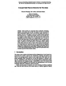
3. Spectral Feature Selection Given a set of pairwise instance similarity S, a graph G can be constructed to represent it. And the target concept specified in S is usually reflected by the structure of G (Chapelle et al., 2006). A feature that is consistent with the graph structure assigns similar values to instances that are near each other on the graph. As shown in Figure 1, feature F assigns values to instances consistently with the graph structure, but F 0 does not. Thus F is more relevant with the target concept and can separate the data better (forms groups with similar instances according to the target concept). According to graph theory, the structure information of a graph can be obtained from its spectrum. Spectral feature selection studies how to select features according to the structures of the graph induced from S. In this work we employ the spectrum of the graph to measure feature relevance and elaborate how to realize spectral feature selection. feature vector

f of feature F

separate data using

feature vector

f

C1

f ' of feature F'

separate data using

f'

C1 '

C2

(a)

C2 '

(b)

Figure 1. Consistency comparison of features. The target concept is represented by the graph structure (clusters indicated by the ellipses). Different shapes denote different values assigned by a feature.

3.1. Ranking Features on Graph We formalize the above idea using the concept of normalized cut for graph, derive two improved functions


from the normalized cut function with the spectrum of the graph, and extend the three functions to their more general forms. These pave the way for constructing the unified framework proposed in this paper.

Theorem 3 Let (λj , ξj ), 0 ≤ j ≤ n − 1 be the eigensystem of L, and αj = cos θj where θj is the angle between fi and ξj . Equation (5) can be rewritten as:

Evaluating Features via Normalized Cut

ϕ1 (Fi ) =

Given a graph G, the Laplacian matrix of G is a linear operator on vectors f = (f1 , f2 , . . . , fn )T ∈ Rn : 1 X < f , Lf >= f Lf = wij (xi − xj )2 2 v ∼v T

i

(4)

j

The equation quantifies how much f varies locally or how “smooth” it is over G. More specifically, the smaller the value of < f , Lf >, the smoother the vector f on G. A smooth vector f assigns similar values to the instances that are close to each other on G, thus it is consistent with the graph structure. This observation motivates us to apply L on a feature vector to measure its consistency with the graph structure. Given a feature vector f i and L, two factors affect the value of < f i , Lf i >: the norms of f i and L. The two factors need to be removed, as they do not contain structure information of the data, but can cause the value of < f i , Lf i > to increase or decrease arbitrarily. The two factors can be removed via normalization. As < f i , Lf i >= 1 1 1 1 f Ti Lf i = f Ti D 2 LD 2 f i = (D 2 f i )T L(D 2 f i ). Let 1 fei = (D 2 f i ) denote the weighted feature vector of Fi , e and fb = f i the normalized weighted feature veci

||fei ||

tor. The score of Fi can be evaluated by the following function: T ϕ1 (Fi ) = fbi L fbi

(5)

Theorem 2 ϕ1 (Fi ) measures the value of the normalized cut (Shi & Malik, 1997) by using fi as the soft cluster indicator to partition the graph G. Proof The theorem holds as: T f T Lf i ϕ1 (Fi ) = fbi L fbi = iT f i Df i

¤

n−1 X

where

j=0

n−1 X

αj2 = 1

(6)

j=0

Proof: Let Σ = Diag(λ0 , λ1 , . . . , λn−1 ) and U = (ξ0 , T ξ1 , . . . , ξn−1 ). As ||fb || = ||ξj || = 1, we have fb ξj = i

i

T cos θj . We can rewrite fbi L fbi as:

T T fbi Lfbi = fbi U ΣU T fbi

= (α0 , . . . , αn−1 )Σ(α0 , . . . , αn−1 )T = Also

Pn−1 j=0

n−1 P i=0

αi2 λi

αj2 = 1, as U U T = I and ||fbi || = 1

¤

Theorem 3 says that using Equation (5), the score of Fi is calculated by combining the eigenvalues of L, and cos θ1 , . . . , cos θn−1 are the combination coefficients, which measures the similarity between the the feature vector and the eigenvectors. According to spectral clustering theories (Ng et al., 2001), the eigenvalues of L measure the separability of the components of the graph1 and the eigenvectors are the corresponding soft cluster indicators (Shi & Malik, 1997). Since λ0 = 0, Equation (6) can be rewritten Pn−1 T as fbi L fbi = j=1 αj2 λj , meaning the value obtained from Equation (5) measures the graph separability by using fbi as the soft cluster indicator, and the separability is estimated by measuring the similarities beb tween L. Since Pn−1 f i2 and those nontrivial eigenvectors Pn−1 of 2 α = 1 and α ≥ 0, we have α ≤ 1, and 0 j j j=0 j=1 Pn−1 2 2 the bigger the α0 , the smaller the j=1 αj . The value of ϕ1 (Fi ) can be small, if fbi is very similar with ξ0 . However, in this case, a small ϕ1 (Fi ) value does not indicate better separability, since the trivial eigenvector ξ0 only carries density information around instances and does not determinePseparability. To handle this n−1 case, we propose to use j=1 αj2 to normalize ϕ1 (Fi ), which gives us the following ranking function:

Ranking Features Using Graph Spectrum Given the normalized Laplacian matrix L, we calculate its spectral decomposition (λi , ξi ), where λi is the eigenvalue and ξi is the eigenvector (0 ≤ i ≤ n − 1). Assuming λ0 ≤ λ1 ≤ . . . ≤ λn−1 , according to Theo1 rem 1, we have: λ0 = 0 and ξ0 = D 2 e. (λ0 , ξ0 ), which is usually called the trivial eigenpair of the graph. Also we can show that all the eigenvalues of L are contained in [0, 2]. Given the spectral decomposition of L, we can rewrite Equation 5 using the eigensystem of L.

αj2 λj ,

n−1 P

ϕ2 (Fi ) =

j=1

αj2 λj

n−1 P j=1

= αj2

T fbi L fbi T 1 − fbi ξ0

(7)

A small ϕ2 (Fi ) indicates that fbi aligns closely to those nontrivial eigenvectors with small eigenvalues, hence 1 The separability is associated with inter-cluster dissimilarity, and the smaller the cut values the better.


provides good separability. According to spectral clustering theory, the leading k eigenvectors of L form the optimal soft cluster indicators that separate G into k parts. Therefore, if k is known, we can also use the following function for ranking: ϕ3 (Fi ) =

k−1 X

(2 − λj )αj2

(8)

j=1

By its definition, ϕ3 assigns bigger scores to features which offer better separability because achieving a big score entails that a feature aligns closely to nontrivial eigenvectors ξ1 , . . . , ξk−1 , with ξ1 having the highest priority. By focusing on only the leading eigenvectors, ϕ3 achieves an effect of reducing noise. This is similar to the mechanism used in Principle Component Analysis. An Extension for Feature Ranking Functions Laplacian matrix is also used by graph based learning models for designing regularization functions to penalize predictors that vary abruptly among adjacent vertices on graph. Smola and Kondor (2003) relate the eigenvectors of L to a Fourier basis extend the Pand n−1 T usage of L to γ(L), where γ(L) = γ(λ j )ξj ξj . j=0 In the formulation, γ(λj ) is an increasing function that penalizes high frequency components2 . As shown in (Zhang & Ando, 2006), γ(λj ) can be very helpful in a noisy learning environment. In the same spirit, we extend our feature ranking functions to the following:

3.2. SPEC- the Framework The proposed framework is built on spectral graph theory. In the framework, the relevance of a feature is determined by its consistency with the structure of the graph induced from S. The three feature ranking functions (ϕ b1 (·), ϕ b2 (·) and ϕ b3 (·)) lay the foundation of the framework and enable us to derive families of supervised and unsupervised feature selection in a unified manner. We realize the unified framework in Algorithm 1. It selects features in three steps: (1) building similarity set S and constructing its graph representation (Line 1-3); (2) evaluating features using the spectrum of the graph (Line 4-6); and (3) ranking features in descending order in terms of feature relevance3 (Line 7-8). We name the framework SPEC, stemming from the SPECtrum decomposition of L. Algorithm 1: SPEC Input: X, γ(·), k, ϕ b ∈ {ϕ b1 , ϕ b2 , ϕ b3 } Output: SFSP EC - the ranked feature list 1 construct S, the similarity set from X (and Y ); 2 construct graph G from S; 3 build W, D and L from G; 4 for each feature vector fi do 1 2 fb ← D 1 f i ; SFSP EC (i) ← ϕ(F b i ); 5 6 7 8

T ϕ b1 (Fi ) = fbi γ(L) fbi =

n−1 X

αj2 γ(λj )

ϕ b2 (Fi ) =

j=1

αj2 γ(λj )

n−1 P j=1

ϕ b3 (Fi ) =

k−1 X

= αj2

T fbi γ(L) fbi T

1 − fbi ξ0

(γ(2) − γ(λj ))αj2

||D 2 f i ||

end ranking SFSP EC in ascending order for ϕ b1 and ϕ b2 , or descending order for ϕ b3 ; return SFSP EC ;

(9)

j=0 n−1 P

i

(10)

(11)

j=1

Calculating the spectral decomposition of L can be expensive for data with a large number of instances. However, since γ(·) is usually a rational function, γ(L) can be calculated efficiently by regarding L as a variable and apply γ(·) on it. For example, assume γ(λ) = λ2 , then γ(L) = L2 . For ϕ b3 (·), the k−1 leading eigenpairs of L can be obtained efficiently by using fast eigen-solvers such as the Implicitly Restarted Arnoldi method (Lehoucq 2001). 2 Here λj is used to estimate frequency, as it measures how much the corresponding basis ξj varies on the graph.

The time complexity of SPEC largely depends on the cost of building the similarity matrix and the calculation of γ(·). If we use the RBF function to build the similarity matrix and γ(·) is in the form of Lr , the time complexity of SPEC can be obtained as follow. First, we need O(mn2 ) operations to build S, W, D, L and L. And we need O(rn3 ) operations to calculate γ(L). Next, we need O(n2 ) operations to calculate SFSP EC (i) for each feature: transforming f i to fbi requires O(n) operations; calculating using ϕ b1 , ϕ b2 and ϕ b2 need O(n2 ) operations4 . Therefore, we need O(mn2 ) operations to calculate scores for m features. Last, we needs O(m log m) operations to rank the features. Hence, the ¡ ¢ overall ¡ time ¢ complexity of SPEC is O (rn + m)n2 , or O mn2 if γ(·) is not used. 3

Features selection is accomplished by choosing the desired number of features from the returned feature list. 4 For ϕ b3 , using Arnoldi method to calculate a few eigenpairs of a large sparse matrix needs roughly O(n2 ) operations, and calculating ϕ b3 itself needs O(k) operations.


3.3. Spectral Feature Selection via SPEC The framework SP EC allows for different similarity matrix measures, γ(·), and ranking function ϕ(·). b It can generate a range of spectral feature selection algorithms for both unsupervised and supervised learning. Hence, SPEC is a general framework for feature selection. To demonstrate the generality and usage of the framework, we show that (1) some existing powerful feature selection algorithms, such as ReliefF and Laplacian Score, can be derived from SPEC as special cases, and (2) novel spectral feature selection algorithms can be derived from SPEC conveniently. Connections to Existing Algorithms The connections of the framework to Laplacian Score and ReliefF are shown in the following two theorems. Theorem 4 Unsupervised feature selection algorithm Laplacian Score (He et al., 2005) is a special case of SPEC, by setting ϕ(·) b = ϕ b2 (·), γ(L) = L and using weighted k-nearest neighborhood graph obtained from RBF kernel function for measuring similarities. Proof: It suffices to show that the ranking function used by Laplacian Score is equivalent to ϕ b2 (·), with γ(L) = L. The ranking function of Laplacian score is: SL =

T fe Lfe

T e = f − f De e. , where f T eT De fe Dfe

=

(f T De)2 eT De 1

1

(D 2 f )T L(D 2 f )

=

Ã

1

1

(D 2 f )T (D 2 f )−

As ξ0 =

1

D2e

1 ||D 2

e||

and fb =

!2 1 1 (D 2 f )T (D 2 e) 1 1 (D 2 e)T (D 2 e)

1

D2f 1

||D 2 f ||

fb L fb T

1 − fb ξ0

Here we use Euclidean distance to calculate the difference between two feature values and use all training data to train ReliefF. According to the design of W , it is easy to verify that D = I. Using Theorem 1, we can show that f T Lf is equivalent to the above ranking function up to a constant factor. Since all features are norm 1 and D = I, we have fb = f . ¤ Note that the similarity matrix defined in Theorem 5 is not positive definite. Therefore the first eigenvalue of L is not 0, which may cause ϕ b2 (·) and ϕ b3 (·) fail. Theorems 4 and 5 establish connection between the two seemingly different feature selection algorithms by showing that they all try to select features that provide the best separability for data according to the given instance similarities.

, we have:

T

SL =

CL6=yi

The framework can also be used to systematically derive novel spectral algorithm by using different S, γ(·) and ranking functions ϕ(·). b For example, given the options of S, γ(·) in Table 1, we can generate families of new supervised and unsupervised feature selection algorithms. We will conduct experiments to evaluate how effective these algorithms are and how they fare in comparison with the baseline algorithms: Laplacian Score and ReliefF.

f T Lf f T Df −

Proof: Under the assumptions, the feature ranking function of ReliefF is equivalent to:   k P 2 (f − f ) M (CL)j k n X  X j=1 i X 1   (fi − fHj )2 −   k (c − 1)k   i=1 j=1

Deriving Novel Algorithms from SPEC

Substituting fe in SL and applying Theorem 1: SL

Here, xj ∈ knn(xi ) indicates xj is one of the k nearest neighbors of xi .

=ϕ b2 (·)

¤

Theorem 5 Assuming the training data has c classes with t instances in each class and all features have been normalized to have unit norm. Supervised feature selection algorithm ReliefF (Robnik-Sikonja & Kononenko, 2003) is a special case of SPEC by setting ϕ(·) b =ϕ b1 (·), γ(L) = L and defining W as:  1 i=j  1 i 6= j, Yi = Yj , xj ∈ knn(xi ) wi,j = k  −1 i 6= j, Yi 6= Yj , xj ∈ knn(xi ) (c−1)k (12)

ϕ(·) b γ(·) Su Ss

ϕ b1 (·), ϕ b2 (·) and ϕ b3 (·) γ(r) = r, γ(r) = r4 RBF kernel function, Diffusion kernel function Similarity matrix defined in Equations 2 and 12

Table 1. The components for SPEC tried in this paper. Su and Ss stand for S used in unsupervised and supervised feature selection respectively.

4. Empirical Study We empirically evaluate the performance of SP EC. In the experiments, we compared the algorithms specified in Table 1 with Laplacian Score (unsupervised) and ReliefF (supervised). Laplacian Score and Re-


liefF are both state-of-the-art feature selection algorithms, comparing with them enables us to examine the efficacy of the algorithms derived from SPEC. We implement SP EC with the spider toolbox5 . 4.1. Data Sets Four benchmark data sets are used for experiments: Hockbase6 , Relathe6 , Pie10p7 and Pix10p8 . Hockbase & Relathe are text data sets generated from the 20-new-group data: Baseball vs. Hockey (Hockbase) and (2) Religion vs. Atheism (Relathe). Pie10p & Pix10p are face image data sets containing 10 persons in each. And we subsample the images down to a size of 100×100 = 10000.

Data Set Hockbase Relathe Pie10p Pix10p

Instance 1993 1427 210 100

Feature 8298 8298 10000 10000

Classes 2 2 10 10

Table 2. Summary of four benchmark data sets

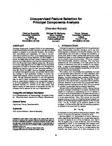
4.2. Evaluation of Selected Features We apply 1-nearest-neighbor (1NN) classifier on data sets with selected features, and use its accuracy to measure the quality of the feature set. All results reported in the paper are obtained by averaging the accuracy from 10 trials of experiments. Study of Unsupervised Cases In the experiment, we use weighted 10-nearest neighborhood graph to represent the similarity among instances. The first two columns of Figure 2 are the 8 plots of accuracy vs. different numbers of selected features, different ranking functions, different γ(·) and different similarity measures. As shown in the plots, in most cases, the majority of the algorithms proposed in Table 1 work better than Laplacian score. Using the diffusion kernel function (Kondor & Lafferty, 2002), SPEC achieves better accuracy than using RBF kernel function. Generally, the more features we select, the better accuracy we can achieve. However, in many cases, this trend is less pronounced when more than 40 features are selected. Using ϕ b2 (·), L and the RBF kernel function, SPEC works exactly the same as Laplacian Score, as expected in our theoretical analysis. Table 3 shows the accuracy when 100 features 5

http://www.kyb.tuebingen.mpg.de/bs/people/spider/ 6 http://people.csail.mit.edu/jrennie/20Newsgroups/ 7 http://www.ri.cmu.edu/projects/project 418.html 8 http://peipa.essex.ac.uk/ipa/pix/faces/manchester/

are selected: the differences between Laplacian Score and the algorithms performing best on each data set are: 0.17 for Hockbase, 0.08 for Relathe, 0.18 for Pie10p and 0.06 for Pix10p. A trend can be observed in the table is that ϕ b1 (·) performs well on the two text data sets, which contain binary classes; ϕ b3 (·) performances well on the two face image data sets, which contain 10 different classes, while ϕ b2 (·) works robustly in both cases. We also observed that comparing with using L, using L4 never downgrades performance significantly, while in certain cases, applying it can improve the performance by a big margin. We averaged the accuracy over different numbers of selected features, different data sets, different similarity measures. Results show that (ϕ b2 , r4 ) works best on benchmark data sets with an averaged accuracy of 0.69 which is followed by (ϕ b3 , r4 ) with an average accuracy of 0.68. The averaged accuracy of Laplacian score is 0.62.

RBF DIF RBF DIF RBF DIF RBF DIF

HOCKBASE (Laplacian Score = 0.58) ϕ b1 , r ϕ b1 , r4 ϕ b2 , r ϕ b2 , r4 ϕ b3 , r ϕ b3 , r4 0.61 0.61 0.58 0.58 0.60 0.60 0.74 0.74 0.75 0.74 0.70 0.70 RELATHE (Laplacian Score = 0.59) ϕ b1 , r ϕ b1 , r4 ϕ b2 , r ϕ b2 , r4 ϕ b3 , r ϕ b3 , r4 0.63 0.63 0.59 0.59 0.55 0.55 0.67 0.67 0.67 0.67 0.61 0.61 PIE10P (Laplacian Score = 0.74) ϕ b1 , r ϕ b1 , r4 ϕ b2 , r ϕ b2 , r4 ϕ b3 , r ϕ b3 , r4 0.75 0.75 0.74 0.78 0.87 0.86 0.81 0.81 0.92 0.91 0.91 0.91 PIX10P (Laplacian Score = 0.88) ϕ b1 , r ϕ b1 , r4 ϕ b2 , r ϕ b2 , r4 ϕ b3 , r ϕ b3 , r4 0.78 0.78 0.88 0.94 0.93 0.91 0.79 0.79 0.84 0.85 0.93 0.92

Table 3. Study of unsupervised cases: comparison of accuracy with 100 selected features. DIF stands for diffusion kernel, and bold typeface indicates the best accuracy.

Study of Supervised Cases Due to the space limit, we skip γ(·) = r4 for supervised feature selection9 . The last column of Figure 2 shows the 4 plots for supervised feature selection. Table 4 shows the accuracy with 100 selected features. From the results we can observe (1) generally supervised feature selection algorithms perform better than unsupervised feature selection algorithms, as they use label information; and (2) ϕ b2 (·) works robustly with both similarity matrix. We averaged the accuracy over different numbers of selected features and different data 9

Also, the similarity matrix defined in Equation 2 is a block matrix with rank k. It can be verified that in this case the first k eigenvalues of L are 0 and the others are 1. Hence, varying γ(·) will not affect the values of the three feature ranking functions.


sets. Results show that using ϕ b2 and the similarity matrix defined in Equation 2, SPEC performs best with averaged accuracy of 0.82, followed by ReliefF whose accuracy is 0.81.

6. Acknowledgements

Experiment results on the benchmark data sets confirm the efficacy of SPEC for both supervised and unsupervised feature selection. Here, we summarize our observations as a guideline for configuring SPEC: basically, if the number of classes is small, use ϕ1 and ϕ2 , otherwise use ϕ2 and ϕ3 . Furthermore, for noisy data, use ϕ3 . Modifying the spectrum with an increasing function also helps remove noise.

References

RLF 0.74 0.73 0.97 0.97

R, ϕ b1 0.74 0.73 0.97 0.97

R, ϕ b2 0.80 0.68 0.97 0.97

R, ϕ b3 0.57 0.53 0.99 0.82

C, ϕ b1 0.69 0.65 0.97 0.95

C, ϕ b2 0.78 0.73 0.97 0.97

C, ϕ b3 0.63 0.64 0.98 0.97

Table 4. Study of supervised cases: comparison of accuracy with 100 selected features. The rows are the results for HOCKBASE, RELATHE, PIE10P and PIX10P, respectively. RLF stands for ReliefF, C and R stand for the similarity matrix defined in Equations 2 and 12 respectively.

5. Discussions and Conclusions Feature selection algorithms can be either supervised or unsupervised (Liu & Yu, 2005). Recently, an increasing number of researchers paid attention to developing unsupervised feature selection. One piece of work closely related to this work is (Wolf & Shashua, 2005). The authors proposed an unsupervised feature selection algorithm based on iteratively calculating the soft cluster indicator matrix and the feature weight vector. They then extended the algorithm to handling data with class labels. Since the input of the algorithm restricts to covariance matrix, it does not handle general similarity matrix and cannot be extended as a general framework for designing new feature selection algorithms and covering existing algorithms. In this paper, we propose a general framework of spectral feature selection for both supervised and unsupervised learning, which facilitates the joint study of supervised and unsupervised feature selection. We show that some powerful existing feature selection algorithms can be derived as special cases from the framework; and families of new effective algorithms can also be derived. Extensive experiments exhibit the generality and usability of the proposed frame. Our work is based on general similarity matrix. It is natural to extend the framework with existing kernel and metric learning methods (Lanckriet et al., 2004) for handling a variety of applications. Another line of our future work is to study semi-supervise feature selection (Zhao & Liu, 2007) using this framework.

The authors would like to express their gratitude to Jieping Ye for his helpful suggestions.

Chapelle, O., Sch¨olkopf, B., and Zien, A. (Eds.) (2006). Semi-supervised learning, chapter GraphBased Methods. The MIT Press. Chung, F. (1997). Spectral graph theory. AMS. Dy, J., & Brodley, C. E. (2004). Feature selection for unsupervised learning. JMLR., 5, 845–889. Guyon, I., & Elisseeff, A. (2003). An introduction to variable and feature selection. JMLR., 3, 1157–1182. He, X., Cai, D., & Niyogi, P. (2005). Laplacian score for feature selection. In NIPS. MIT Press. Kondor, R. I., & Lafferty, J. (2002). Diffusion kernels on graphs and other discrete structures. ICML. Lanckriet, G. R. G., Cristianini, N., Bartlett, P., Ghaoui, L. E., & Jordan, M. I. (2004). Learning the kernel matrix with semidefinite programming. JMLR., 5, 27–72. Liu, H., & Yu, L. (2005). Toward integrating feature selection algorithms for classification and clustering. IEEE TKDE, 17, 491–502. Ng, A., Jordan, M., & Weiss, Y. (2001). On spectral clustering: Analysis and an algorithm. NIPS. Lehoucq, R. B. (2001). Implicitly Restarted Arnoldi Methods and Subspace Iteration. SIAM J. Matrix Anal. Appl. 23, 551–562. Robnik-Sikonja, M., & Kononenko, I. (2003). Theoretical and empirical analysis of Relief and ReliefF. Machine Learning, 53, 23–69. Shi, J., & Malik, J. (1997). Normalized cuts and image segmentation. CVPR. Smola, A., & Kondor, I. (2003). Kernels and regularization on graphs. COLT. Wolf, L., & Shashua, A. (2005). Feature selection for unsupervised and supervised inference: The emergence of sparsity in a weight-based approach. JMLR., 6, 1855–1887. Zhang, T., & Ando, R. (2006). Analysis of spectral kernel design based semi-supervised learning. NIPS. Zhao, Z., & Liu, H. (2007). Semi-supervised Feature Selection via Spectral Analysis. SDM.

Spectral Feature Selection for Supervised and Unsupervised Learning Data Set: HOCKBASE, Similarity: RBF

Data Set: HOCKBASE (SUPERVISED)

Data Set: HOCKBASE, Similarity: diffusion

0.75

0.75

0.9

LAPLACIAN F1 + r F1 + r4 F2 + r

0.7

F2 + r4 F3 + r

0.65

0.8

0.7

0.7 0.65

F3 + r4

0.6 0.6

ReliefF R + F1 R + F2 R + F3 C + F1 C + F2 C + F3

0.6 0.5

0.55

0.5 10

0.55

20

30

40

50

60

70

80

90

100

0.5 10

0.4

20

Data Set: RELATHE, Similarity: RBF

40

50

60

70

80

90

100

0.68

0.68

0.66

F1 + r4 F2 + r

0.66

F2 + r4 F3 + r

0.62

0.6

0.58

0.58

0.56

0.56

0.54

0.54

0.52

0.52 40

40

50

60

70

80

90

100

0.75

0.7

0.62

F3 + r4

30

30

0.64

0.6

20

20

Data Set: RELATHE (SUPERVISED)

0.7 LAPLACIAN F1 + r

0.64

0.3 10

Data Set: RELATHE, Similarity: diffusion

0.7

0.5 10

30

50

60

70

80

90

100

0.5 10

0.65


0.6

0.55

20

Data Set: PIE10P, Similarity: RBF

30

40

50

60

70

80

90

100

0.5 10

20

Data Set: PIE10P, Similarity: diffusion

30

40

50

60

70

80

90

100

Data Set: PIE10P (SUPERVISED) 1

0.9

0.9

0.85

0.85

0.8

0.8

0.75

0.75

0.7

0.7

0.65

0.45 0.4 10

0.55

4

F2 + r F3 + r

0.5

F3 + r 30

40

50

60

70

80

0.8

0.5 0.45

4

20


0.85

0.6

F1 + r4 F2 + r

0.55

0.9

0.65

LAPLACIAN F1 + r

0.6

0.95

90

100

0.4 10

20

Data Set: PIX10P, Similarity: RBF

30

40

50

60

70

80

90

100

0.75 10

20

Data Set: PIX10P, Similarity: diffusion

1

1

0.9

0.9

0.8

0.8

30

40

50

60

70

80

90

100

Data Set: PIX10P (SUPERVISED) 1

0.9

0.8

0.7 0.7

0.7

LAPLACIAN F1 + r

0.6


4

F1 + r F2 + r

0.6

0.5 10

0.4 0.5

F3 + r4 20

30

40

50

60

70

80

0.5

0.6

F2 + r4 F3 + r

90

100

10

20

30

40

50

60

70

80

90

100

10

20

30

40

50

60

70

80

90

100

Figure 2. Accuracy (X axis) vs. different numbers of selected features (Y axis), different feature ranking functions, different γ(·) and different similarity measures. Each row stands for a different data set. The first two columns are for unsupervised feature selection and the last column is for supervised feature selection. Thick lines in the figures are for the baseline feature selection algorithms: Laplacian Score and ReliefF. In the legend, F 1, F 2 and F 3 stand for feature ranking function ϕ b1 (·), ϕ b2 (·) and ϕ b3 (·); C and R stand for the similarity matrix defined in Equations 2 and 12.