May 8, 2014 - T FUT and with compact Fs â F is equal to the index of T, up to a sign. .... rFs + (1 â r)Fs is a homotopy in Î(F, U) keeping the initial and final ...
Spectral flows of dilations of Fredholm operators
arXiv:1405.0410v2 [math-ph] 8 May 2014
Giuseppe De Nittis, Hermann Schulz-Baldes Department Mathematik, Universit¨at Erlangen-N¨ urnberg, Germany
Abstract Given an essentially unitary contraction and an arbitrary unitary dilation of it, there is a naturally associated spectral flow which is shown to be equal to the index of the operator. This result is interpreted in terms of the K-theory of an associated mapping cone. It is then extended to connect Z2 indices of odd symmetric Fredholm operators to a Z2 -valued spectral flow.
The spectral flow of a one-parameter family of self-adjoint Fredholm operators was introduced by Atiyah, Patodi and Singer [APS] and was under certain conditions shown to be connected to indices of Fredholm operators. A particularly convenient technical reformulation was given by Phillips [Phi1] which also extends to unbounded operators [CP]. As this version of spectral flow is also used here, it is reviewed in Section 1 below. The first part of the paper then considers an essentially unitary contraction operator T on a Hilbert space K and an arbitrary unitary dilation UT associated to it, namely a unitary operator on a larger Hilbert space H so that its restriction to K is T . If P is the projection onto K and one sets F = 2P − 1, then Theorem 2 in Section 2 shows that the spectral flow of any path s ∈ [0, 1] 7→ Fs from F to UT∗ F UT and with compact Fs − F is equal to the index of T , up to a sign. Two proofs are provided, one by a homotopy argument and one using indices of pairs of projections [Kat, ASS]. This result already appears in [Phi2], but for sake of completeness and as preparation for the second part of the paper, we provide two proofs of it. Inspired by [Put, CPR], Section 3 then provides a K-theoretic interpretation of the theme index = spectral flow based on a mapping cone exact sequence and the pairing of its K-groups with adequate Fredholm modules. Indeed, the exposition shows that there is a tight connection between unitary dilations and Fredholm modules. More novel is an extension of the above result to essential untaries operators and dilations having symmetry properties linked to a real or quaternionic structure on the Hilbert space. Examples are real, quaterionic, symmetric and anti-symmetric operators. Anti-symmetric operators are in bijection with so-called odd symmetric operators and such Fredholm operators have recently been shown to have Z2 indices given by the dimension of their kernel modulo 2 [SB]. All this is reviewed in Section 4. Let us also note that these Z2 indices are defined for 1
a much wider class of Fredholm operators than considered by Atiyah and Singer [AS] which required the anti-symmetric Fredholm operators also to be real. In Section 5 a Z2 -valued spectral flow is defined for paths with an adequate symmetry property. The basic idea leading to this definition is already contained in the analysis of Z2 invariants of edge states in quantum systems with odd time-reversal symmetry [ASV]. In Section 6 this Z2 -valued spectral flow of an odd symmetric dilation is again shown to be equal to the Z2 index of the dilated Fredholm operator. A mapping cone interpretation with the flavor of Real K-theory [Sch] is sketched in the final Section 7. Our motivation to revisit the problem of spectral flow and to extend it to Z2 indices stems from applications to solid state physics. This will be the subject of a companion paper [DS]. Acknowledgement: We thank Magnus Goffeng for correcting several mistakes in a first version of the manuscript. We received financial support of the DFG and the Alexander von Humboldt Foundation.
1
Spectral flow of a pair of unitary equivalent operators
In order to fix notations and terminology, this section reviews some standard facts from the theory of Fredholm operators on a separable Hilbert space H as well as the notion of spectral flow. Let B(H), K(H) and F(H) denote the sets of bounded, compact and Fredholm operators on H, respectively. Recall that F ∈ B(H) is Fredholm if and only if it has closed range T H and finite-dimensional kernel Ker(F ) and cokernel Ker(F ∗ ). Atkinson’s theorem states that Fredholm operators are the invertibles modulo compact perturbation and this provides the following characterization � F(H) = F ∈ B(H) | ∃ S ∈ B(H), K1 , K2 ∈ K(H) with SF − K1 = 1 = F S − K2 . In particular, the property to be Fredholm is invariant under compact perturbations. Furthermore, F(H) is an open subset of B(H) which is closed under the adjoint involution. The Noether index of a Fredholm operator F is defined by Ind(F ) = dim(Ker(F )) − dim(Ker(F ∗ )) ∈ Z. The index is a homotopy invariant that is stable under compact perturbations, namely Ind(F ) = Ind(F + K) for all K ∈ K(H). Moreover, Fn (H) = Ind−1 (n) is a path connected component for any n ∈ Z so that the index map Ind : S F(H) → Z establishes a bijection between Z and the path-connected components of F(H) = n∈Z Fn (H). The set F(H) has a group structure under the multiplication of operators and the index map is a group homomorphism onto the additive group Z. Let SF(H) = {F ∈ F(H) | F = F ∗ } be the subset of self-adjoint Fredholm operators. Equivalently, SF(H) = {F ∈ B(H) | F = F ∗ and 0 6∈ σess (F )} where σess (F ) denotes the essential spectrum. Although SF(H) ⊂ F0 (H), the space SF(H) has a non-trivial topology. First of all, it has three disjoint components: � � SF± (H) = F ∈ SF(H) | σess (F ) ⊂ R± , SF∗ (H) = F ∈ SF(H) | σess (F ) ∩ R± 6= ∅ ,
2
Figure 1: Schematic representation of the objects used in the definition (1) of the spectral flow as well as in the second proof of Theorem 2. Far from the crossings it is possible to set a = b = 0.
where the notation R± = {x ∈ R | ± x > 0}� was used. The two components SF± (H) are contractible [AS, Theorem B], but π1 SF∗ (H) ∼ = Z via the spectral flow isomorphism. The spectral flow was introduced in [APS] using the intuitive notion of intersection theory of spectral curves. Here we rather work with the versatile, but equivalent notion of spectral flow proposed in [Phi1]. Let s ∈ [0, 1] 7→ Fs ∈ SF∗ (H) be a continuous path, not necessarily closed. For a ∈ (−1, 0] and b ∈ [0, +1) set Qa,b (s) = χ(a,b] (Fs ) , where χI denotes the characteristic function on I ⊂ R. By compactness (see Figure 1 where σess (F ) = {−1, 1} is assumed), it is possible to choose a finite partition 0 = s0 < s1 < . . . < sN −1 < sN = 1 of [0, 1] and an < 0 < bn , n = 1, . . . , N , such that s ∈ [sn−1 , sn ] 7→ Qan ,bn (s) is continuous with constant (necessarily) finite rank. Then define the spectral flow by Sf(s ∈ [0, 1] 7→ Fs ) =
N X
TrH (Qan ,0 (sn−1 ) − Qan ,0 (sn )) .
(1)
n=1
Note that Qan ,0 (sn−1 ) and Qan ,0 (sn ) are both finite dimensional projections so that the trace is finite. The basic result about the spectral flow is that it is well-defined by the above procedure and it is homotopy invariant. A detailed proof can be found in [Phi1]. Theorem 1 The definition of Sf(s ∈ [0, 1] 7→ Fs ) is independent of the choice of the partition 0 = s0 < s1 < . . . < sN −1 < sN = 1 of [0, 1] and values an < 0 < bn such that s ∈ [sn−1 , sn ] 7→ Qan ,bn (s) is continuous. Moreover, let s ∈ [0, 1] 7→ Fs and s ∈ [0, 1] 7→ Gs be two continuous paths in SF∗ (H) such that F0 = G0 and F1 = G1 . Then Sf(s ∈ [0, 1] 7→ Fs ) = Sf(s ∈ [0, 1] 7→ 3
Gs ) if and only if there exists a norm continuous homotopy between the two paths leaving the endpoints fixed. Remark Let us briefly sketch the connection of definition (1) to the intuitive notion of spectral flow. By standard perturbation theory arguments [Kat], it is possible to label the spectral curves λj (s) such that each varies continuously in s. When s increases the spectral curves s 7→ λj (s) can cross the segment [0, 1] × {0}. One has a spectral crossing of positive signature if there is a passage from a negative to a positive eigenvalue or a spectral crossing of negative signature if the passage is from a positive to a negative eigenvalue. If there is a finite number of crossings and no crossings at the boundaries s = 0 and s = 1, the sum of these signatures over all crossings is equal to Sf(s ∈ [0, 1] 7→ Fs ). The advantage of definition (1) is that the boundaries do not require special treatment and that there may well be an infinite number of crossings. � � When Theorem 1 is applied to closed paths, it shows that Sf : π1 SF∗ (H) → Z is a welldefined group homomorphism. To verify that this map is bijective, one can use the fact that the space � c ∗ (H) = F ∈ SF∗ (H) | kF k = 1 , σess (F ) = {−1, 1} SF c ∗ (H) → U∗ (H) defined by is a deformation retract of SF∗ (H) and that the map ϕ : SF ıπ(F +1) ϕ(F ) = e is an homotopy equivalence [AS]. Here U∗ (H) is the subgroup of those unitary � operators U ∈ U(H) for which U − 1 ∈ K(H). The sequence of isomorphisms π1 SF∗ (H) ∼ = � � � c ∗ (H) ∼ π1 SF = π1 U∗ (H) combined with the standard isomorphism π1 U∗ (H) → Z given by the winding number concludes the description of the fundamental group of SF∗ (H). Just for sake of completeness let us recall that the winding number of a differentiable loop s ∈ [0, 1] 7→ Us ∈ U∗ (H) is given by Z 1 � 1 ds Tr (Us )−1 ∂s Us , Wind(s ∈ [0, 1] 7→ Us ) = 2πı 0 whenever ∂s Us is traceclass. For adequate paths, the equality Sf(s ∈ [0, 1] 7→ Fs ) = Wind(s ∈ [0, 1] 7→ ϕ(Fs )) provides an alternative formula for the computation of the spectral flow. c ∗ (H). Given F ∈ SF c ∗ (H) Focus here will be on the spectral flow of certain special paths in SF and a unitary U ∈ U(H), let Θ(F, U ) denote the set of paths s ∈ [0, 1] 7→ Fs such that (i) (ii) (iii)
F0 = F , Fs − F ∈ K(H) for all s ∈ [0, 1] , F1 = U ∗ F U .
(2)
Note that σ(F1 ) = σ(F0 ). The spectral flow Sf(s ∈ [0, 1] 7→ Fs ) of such a path is well-defined and equal to the spectral flow of the path obtained by concatenation with the isospectral path r ∈ [0, 1] 7→ (U r )∗ F U r . Proposition 1 The spectral flow Sf : Θ(F, U ) → Z is equal to a constant denoted by Sf(F, U ). In particular, Sf(F, U ) = Sf(s ∈ [0, 1] 7→ F + s U ∗ [F, U ]) . (3) 4
Proof. Let s ∈ [0, 1] 7→ Fs and s ∈ [0, 1] 7→ Fs0 be two paths in Θ(F, U ). Then r ∈ [0, 1] 7→ rFs + (1 − r)Fs0 is a homotopy in Θ(F, U ) keeping the initial and final point fixed, so that Theorem 1 implies the first claim. The second follows because s ∈ [0, 1] 7→ F + s U ∗ [F, U ] is indeed a path in Θ(F, U ) since U ∗ [F, U ] = F1 − F0 ∈ K(H). 2 Let us introduce the set of operator pairs for which a spectral flow can be defined: n o c P(H) = (F, U ) ∈ SF∗ (H) × U(H) | [F, U ] compact . It carries the subspace topology induced from the norm topology on B(H) × B(H). Note that indeed each point (F, U ) ∈ P(H) defines a class of paths Θ(F, U ) so that it is possible to view the spectral flow as a map Sf : P(H) → Z (strictly speaking this is Sf ◦ Θ). Proposition 2 The spectral flow Sf : P(H) → Z is locally constant. Proof. Let (F (0), U (0)) and (F (1), U (1)) be two points connected by a continuous path r ∈ c ∗ (H), given by r 7→ F (r), [0, 1] 7→ (F (r), U (r)) in P(H). This means that there is a path α in SF c ∗ (H), given by r 7→ U (r)∗ F (r)U (r), which connects F (0) with F (1) and a second path β in SF ∗ ∗ which connects U (0) F (0)U (0) with U (1) F (1)U (1). Let γr ∈ Θ(F (r), U (r)) by any path connecting F (r) to U (r)∗ F (r)U (r) by compact perturbations. For each r ∈ [0, 1] let us denote by αr the reduced path which connects F (0) with F (r) along the path α. In similar way let us introduce also the reduced path βr . The composed paths θr = βr−1 ◦ γr ◦ αr produce a homotopy between θ0 = γ0 and θ1 within the class of paths having same extreme points F (0) and U (0)∗ F (0)U (0). Theorem 1 applies so that Sf(θ1 ) = Sf(θ0 ) = Sf(F (0), U (0)). Now, by applying the composition rule of the spectral flow Sf(θ1 ) = Sf(α) + Sf(γ1 ) − Sf(β) and observing that Sf(α) = Sf(β) one gets Sf(F (0), U (0)) = Sf(γ1 ) = Sf(F (1), U (1)). 2
2
Dilation of a Fredholm operator and its spectral flow
In this section, the index of an arbitrary Fredholm operator is being calculated as a spectral flow, actually of a whole family of spectral flows associated to arbitrary dilations. Let K be a separable Hilbert space. Let T ∈ B(K) be a contraction, namely kT k ≤ 1. A unitary dilation of T is a unitary operator UT ∈ B(H) on some Hilbert space H in which K is isometrically embedded by an injective partial isometry Π : K ,→ H such that T = Π∗ UT Π .
(4)
To exclude a trivial case, it will always be assumed that H K is infinite dimensional. Recall that an operator T is called essentially unitary if T ∗ T − 1 and T T ∗ − 1 are compact operators. The set EU(K) of essentially unitary operators is a subset of the Fredholm operators F(K). Theorem 2 [Phi2] Let UT ∈ U(H) be a unitary dilation of an essentially unitary contraction T ∈ EU(K) and let Π : K ,→ H be the associated injective partial isometry. Then, with c ∗ (H) F = 2 ΠΠ∗ − 1 ∈ SF � Ind(T ) = − Sf(F, UT ) = − Sf s ∈ [0, 1] 7→ F + s UT∗ [F, UT ] . (5) 5
Two proofs will be provided, one by constructing a homotopy to a special dilation for which the identity (5) can be checked by direct computation, and one which uses the index of Fredholm pairs of projections introduced by Kato [Kat] and studied in detail in [ASS]. Proof of Theorem 2 by homotopy. Let H = K ⊕ K0 for some Hilbert space K0 . In this grading, � � � � T B 1 0 UT = , F = , (6) C D 0 −1 with adequate operators B, C and D. By unitarity, BB ∗ = 1 − T T ∗ and C ∗ C = 1 − T ∗ T . As T is essentially unitary, it follows that BB ∗ and C ∗ C are compact and thus also B and C are compact (e.g. by the polar decomposition). This implies that [F, UT ] ∈ K(H). Furthermore, c ∗ (H) and thus by Proposition 1 the spectral flow Sf(F, UT ) is well-defined and the F ∈ SF second equality in (5) holds. Because it was assumed that K0 = H K is infinite dimensional, there exists a unitary map from K to K0 and, as a basis change does not change the spectral flow, one may suppose K = K0 from now on. Actually the infinite dimensionality of K0 follows if Ind(T ) 6= 0. Indeed, by unitarity of UT also D∗ D − 1 = B ∗ B and DD∗ − 1 = CC ∗ are compact, so that D is also an essential unitary operator. Since the index of UT vanishes and the index is stable under compact perturbations, it follows that 0 = Ind(T ⊕ D) = Ind(T ) + Ind(D). But a non-vanishing index only exists in infinite dimension. The basic idea of the proof is to verify (5) for one particular unitary dilation UTH and then to show that any other unitary dilation UT is connected with UTH by a continuous path r ∈ [0, 1] 7→ U (r) which is such that (F, U (r)) ∈ P(H) holds (which is equivalent to the offdiagonal entry of U (r) being compact). By Proposition 1 one then has Sf(F, UT ) = Sf(F, UTH ) and one can conclude that (5) holds for any unitary dilation if only it can be checked for the special dilation UTH . The latter is chosen to be the Halmos dilation [Hal]: 1
T (1 − T T ∗ ) 2 1 −T ∗ (1 − T ∗ T ) 2
� H
UT =
� .
(7)
Let T = V |T | be the polar decomposition with partial isometry V such that Ker(V ) = Ker(T ). Due to the continuous path r ∈ [0, 1] 7→ V |T |r and the stability of the index one has Ind(T ) = Ind(V ). Let us consider the path r ∈ [0, 1] 7→ U (r) with � 1� V |T |r (1 − V |T |2r V ∗ ) 2 U (r) = . 1 (1 − |T |r V ∗ V |T |r ) 2 −|T |r V ∗ Indeed, (F, U (r)) ∈ P(H) and the path connects U (1) = UTH to 1
V (1 − V V ∗ ) 2 1 (1 − V ∗ V ) 2 −V ∗
� U (0) = Now
� .
� � � � 1 0 −(1 − V ∗ V ) 0 F + s U (0) [F, U (0)] = + 2s 0 −1 0 1−VV∗ ∗
6
where one uses that 1 − V ∗ V and 1 − V V ∗ are the orthogonal projections on Ker(V ) = Ker(T ) and Ker(V ∗ ) = Ker(T ∗ ), respectively. These relations also imply that the spectral flow of s ∈ [0, 1] 7→ F + s U (0)∗ [F, U (0)] is equal to −Ind(T ) and therefore the identity (5) for the Halmos dilation follows. It now remains to construct a continuous map from an arbitrary dilation UT to UTH such that, when combined with F , one stays in P(H). For that purpose, let us consider W = (UTH )∗ UT and show that it is homotopic � � to the identity with a path having compact off-diagonal. The matrix A B entries of W = satisfy Ind(A) = Ind(D) = 0 (actually, one also has A = T ∗ T , but this C D is irrelevant in the following) and B and C are compact. Consequently, by standard Fredholm theory there are partial isometries VA and VD such that A + � VA and D + � VD are invertible for � � ∈ (0, 1) sufficiently small such that the path r ∈ [0, �] 7→ W (r) = � � > 0. Now choose A + r VA B remains in the invertibles (the spectrum of W (r) does not touch 0 if C D + r VD r < 1). Next decompose � �� � A + r VA 0 1 (A + r VA )−1 B W (r) = . 0 D + r VD (D + r VD )−1 C 1 The second factor is a compact perturbation of the identity and can therefore be continuously deformed within the compact operators to the identity, e.g. using spectral theory for compact operators. Thus one obtains a path r ∈ [�, 1] 7→ W (r) in the invertibles on K ⊕ K with compact off-diagonal entries connecting W (�) to the identity (as also the invertibles on K are path connected by the polar decomposition). From this path of invertibles one obtains the desired path of unitaries r ∈ [0, 1] 7→ W (r)|W (r)|−1 . Let us note that the homotopy is not a path of unitary dilations of T , but this is not needed in order to connect the spectral flows. 2 Proof of Theorem 2 using Fredholm pairs of projections. (This proof looks shorter than the above, but appeals to several results from [ASS].) Let UT and F be as in (6) and consider any path [0, 1] ∈ s → Fs in Θ(F, UT ), namely such that F0 = F , F1 = UT∗ F UT and Fs − F ∈ K(H) for all s ∈ [0, 1]. Let us start from the definition (1) of the spectral flow. As Qan ,0 (sn−1 ) and Qan ,0 (sn ) are both finite dimensional projections, the difference of their traces can be expressed in terms of the index of a pair of projections. One of the equivalent definitions in [ASS] is Ind(P, Q) = Ind(QP Q) whenever QP Q is a Fredholm operator on QH. With this, Sf(s ∈ [0, 1] 7→ Fs ) =
N X
Ind (Qan ,0 (sn−1 ), Qan ,0 (sn )) .
n=1
Let us consider the orthogonal decomposition P (s) = Qa (s) ⊕ Qa,0 (s) for a < 0. The map [sn−1 , sn ] 3 s 7→ Qan (s) is continuous and for any pair sn−1 6 s01 < s02 6 sn an application of the Riesz integral and of the resolvent identity shows that the difference Qan (s01 ) − Qan (s02 ) is compact and kQan (s01 ) − Qan (s02 )k 6 C kFs01 − Fs02 k. From these two facts together follows that Qan (sn−1 ) and Qan (sn ) are a Fredholm pair with Ind(Qan (sn−1 ), Qan (sn )) = 0 [ASS, Proposition 3.2 and Theorem 3.4(c)]. Since the computation of the index is linear with respect to 7
the orthogonal sum of projections [ASS, Lemma A.9], one has Ind(Qan ,0 (sn−1 ), Qan ,0 (sn )) = Ind(P (sn−1 ), P (sn )). Observing that the difference P (sn−1 ) − P (sn ) is compact, one uses again [ASS, Theorem 3.4(c)] for the sum of the telescopic series: Sf(s ∈ [0, 1] 7→ Fs ) = Ind(P (0), P (1)) = Ind(P (0), UT∗ P (0)UT ) = Ind(P (0)UT P (0)) where the last step is provided by [ASS, Theorem 5.2] and P (0)UT P (0) has to be considered as an operator on P (0)H. Observing that P (0) ⊕ P = 1, with P = χ[0,+∞) (F ) the spectral projection of F on the positive spectrum, one concludes that Ind(P (0)UT P (0)) = −Ind(P UT P ) = −Ind(T ) since P UT P |P H = Π∗ UT Π = T . 2
3
Mapping cone of a Fredholm module
Let A be a C∗ -algebra which is realized as a subalgebra of the bounded operators B(H) on a separable Hilbert space H. Associated are the K-groups K0 (A) and K1 (A) of homotopy classes of projections and unitaries in A. Topological content can be extracted from these groups via pairing with Fredholm modules. The ungraded version of an even bounded Fredholm module (H, F ) for A is a unitary operator F on H such that for all A ∈ A the commutators [F, A] ∈ K(H). An odd bounded Fredholm module is an even bounded Fredholm module (H, F ) c ∗ (H). for which, moreover, F 2 = 1 and σess (F ) = {−1, 1}. Equivalently, the unitary F lies in SF In the literature [Con], even Fredholm modules are always graded, so let us briefly explain the connection as well as the relation between unitary dilations and odd Fredholm modules. b Fb, Γ) for Remark 1 By definition [Con], a (graded version of an) even Fredholm module (H, b Fb) together with a (unitary) grading operator a C∗ -algebra Ab is an odd Fredholm module (H, 2 b and ΓFbΓ = −Fb. Given an ungraded version Γ satisfying Γ = 1, ΓAΓ = A for all A ∈ A, of an even bounded Fredholm module (H, F ) for A, one obtains a graded version by setting b = H ⊗ C2 and Ab = A ⊗ 12 , furthermore setting Fb =