Open Eng. 2016; 6:106–119
Research Article
Open Access
Chetteti RamReddy* and Teegala Pradeepa
Spectral Quasi-linearization Method for Homogeneous-Heterogeneous Reactions on Nonlinear Convection Flow of Micropolar Fluid Saturated Porous Medium with Convective Boundary Condition DOI 10.1515/eng-2016-0015 Received Jan 12, 2016; accepted Apr 17, 2016
Abstract: Based on the nonlinear variation of density with temperature (NDT) in the buoyancy term, the mixed convection flow along a vertical plate of a micropolar fluid saturated porous medium is considered. In addition, the effect of homogeneous-heterogeneous reaction and convective boundary condition has been taken into account. Using lie scaling group transformations, the similarity representation is attained for the system of partial differential equations, prior to being solved by a spectral quasilinearization method. The results show that in the presence of aiding and opposing flow situations, both the species concentration and mass transfer rate decreases when the strength of homogeneous and heterogeneous reaction parameters are enhanced. Keywords: Non-linear convection; Homogeneousheterogeneous reactions; Micropolar fluid; Convective boundary condition; Porous medium; Spectral quasilinearization method
1 Introduction The study of mixed convection, heat and mass transfer embedded in porous media has substantially increased during the past decades, owing to its wide range of applications including thermal insulation, extraction of crude oil and chemical catalytic reactors, and heat exchangers
*Corresponding Author: Chetteti RamReddy: Department of Mathematics, National Institute of Technology, Warangal-506004, India; Email:
[email protected],
[email protected] Teegala Pradeepa: Department of Mathematics, National Institute of Technology, Warangal-506004, India
placed in a low-velocity environments, among others. A comprehensive review of convective heat transfer in Darcy and non-Darcy porous medium can be found in the books by Vafai [1], Ingham and Pop [2] and Nield and Bejan [3]. The characteristics of fluids with suspended particles cannot be successfully interpreted by the theory of Newtonian fluids, leading to many researchers combining these analyses with micropolar fluids. Eringen [4] initiated the theory of micropolar fluids, in which microscopic effects arising from the local structure and micromotion of the fluid elements are taken into consideration. In addition, these fluids can be used to analyze the behavior of exotic lubricants, animal blood, polymer fluids, clouds with dust, sediments in rivers and liquid crystal with rigid molecules, etc. A deep monograph to the discrete aspects of micropolar fluid, along with the applications of these fluids in the theory of lubrication and porous media is reported in the books by Lukaszewicz [5] and Eremeyev et al. [6]. Further the study of micropolar fluids in Darcy and non-Darcy porous medium is presented in Srinivasacharya and Ramreddy [7, 8]. Progress in mixed convection and chemical reactions have been largely devoted to heat and mass transfer problems. With applications including drying, evaporation at the surface of the water body, energy transfer in wet cooling surface and the flow in a desert cooler. Most of the chemical reactions comprise of both homogeneous and heterogeneous reactions. The homogeneous reaction takes place in bulk of the fluid, while heterogeneous reaction occurs on some catalytic surfaces. Generally, the interaction between the homogeneous and heterogeneous reactions are very complex and is involved in the production and consumption of reactant species at various rates, both on the catalytic surfaces and within the fluid. Chaudhary and Merkin [9] explained the homogeneousheterogeneous reactions in boundary layer flow, with in-
© 2016 Ch. RamReddy and T. Pradeepa, published by De Gruyter Open. This work is licensed under the Creative Commons Attribution-NonCommercial-NoDerivs 3.0 License.
Unauthenticated Download Date | 5/23/16 10:53 AM
Nonlinear Convection Flow of Micropolar Fluid. . .
fluence of loss of autocatalyst represented by a dimensionless parameter. Shaw et al. [10] analyzed the effect of homogeneous-heterogeneous reactions on micropolar fluid flow from a permeable stretching or shrinking sheet, including influence of permeability. Kameswaran et al. [11] discussed the stagnation point flow over a shrinking or stretching sheet placed in a saturated porous medium, assessing the effect of homogeneous-heterogeneous reactions. The combined effects of external magnetic field and internal heat generation on heat and mass transfer of nanofluid flow in the presence of homogeneousheterogeneous reactions is examined by Nandkeolyar et al. [12]. The broad research interest in heat transfer problems with convective surface boundary condition is motivated by prominent applications in metal drying, transpiration cooling process, laser pulse heating, current carrying conductor cooled by ambient air, and nuclear fuel rod cooled by a liquid metal coolant etc. In convective boundary condition, heat is supplied to the convecting fluid through a bounding surface with a finite heat capacity, which provides a convective heat transfer coefficient. Makinde and Aziz [13] scrutinized hydro-magnetic mixed convection flow along a vertical plate embedded in a porous medium, with influence of convective boundary condition. In the presence of uniform magnetic field and thermal radiation, the stagnation point flow towards stretching plate in a micropolar fluid with slip velocity and convective boundary condition investigated by Mostafa et al. [14]. Swapna et al. [15] analyzed the mixed convection magneto-micropolar fluid flow along a vertical porous stretching sheet embedded in a Darcy porous medium including influence of radiation, variable viscosity and convective boundary condition. In recent times, Ramreddy et al. [16] presented the spectral quasi-linearization method for the mixed convection flow in a micropolar fluid saturated porous medium with convective boundary condition. In all erstwhile studies, effect of nonlinear convection is neglected. In nonlinear convection, the density temperature relation is nonlinear which causes a nonlinear convective heat transfer. Further, the nonlinear variation in buoyancy may effect on the flow and heat transfer characteristics (for more details see Barrow and Rao [17] and Vajravelu et al. [18]). This physical concept has a wide range of applications in geothermal and engineering such as pore water convection near salt domes, cooling of electric equipment, and the residual warm water discharged from a geothermal power plant. Kameswaran et al. [19] studied the thermophoretic and nonlinear convection flow in non-Darcy porous medium. The convective flow of non-
|
107
linear density-temperature relationship over an impulsive stretching sheet examined by Motsa et al. [20], solving the system of equations by the spectral homotopy analysis method. Nandkeolyar et al. [21] investigated the effect of viscous dissipation on a stagnation point flow of a nanofluid through a stretching sheet, with an influence of nonlinear convection. Motivated by aforementioned papers, the objective of this paper is to analyze the effect of homogeneousheterogeneous reactions on mixed convection flow of a micropolar fluid embedded in porous medium, with the influence of nonlinear convection under convective boundary condition. A spectral quasi-linearization method is employed to solve the system of equations. Also, the physical quantities of the flow and heat transfer coefficient are analyzed in both aiding and opposing flow situations for various parameters namely, the micropolar parameter, nonlinear convection, Darcy parameter and Biot number.
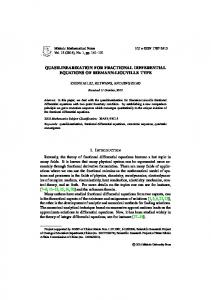
2 Mathematical Formulation Consider the steady, laminar, mixed convective flow of micropolar fluid along a vertical plate embedded in Darcy porous medium. The fluid density is assumed to vary with temperature in nonlinear form. Choose the coordinate system such that the x-axis is along the vertical plate and yaxis normal to the plate. The physical model and coordinate system are shown in Fig. 1. The temperature difference between the plate and the medium are assumed to be large. The velocity of the outer flow is of the form u e , the
Figure 1: Physical model and coordinate system.
Unauthenticated Download Date | 5/23/16 10:53 AM
108 | Ch. RamReddy and T. Pradeepa free stream temperature is T∞ . The plate is either heated or cooled from left by convection from a fluid of temperature T f with T f > T∞ corresponding to a heated surface (assisting flow), and T f < T∞ corresponding to a cooled surface (opposing flow) respectively. Let us assume a simple homogeneous-heterogeneous reaction model exists as proposed by Chaudary and Merkin [9] in the following form: For the homogeneous reaction we took cubic autocatalysis, namely A + 2B → 3B, rate = k c a b
2
A + B → 3B, rate = k s a By employing Boussinesq approximation and making use of the standard boundary layer approximations, the governing equations for the micropolar fluid [22, 23]) are given by: ∂u ∂v + =0 ∂x ∂y (︂
∂u ∂u u +v ∂x ∂y
)︂
∂b D A ∂a ∂y = k s a, D B ∂y = −k s a
x=
ω=
du e 1 ∂2 u ∂ω (µ + κ) 2 + ρu e +κ (2) ε dx ∂y ∂y (︁ )︁ 2 + ρg* β1 (T − T∞ ) + β2 (T − T∞ ) µ (u e − u) Kp
ρj ε
u
∂ω ∂ω +v ∂x ∂y
)︂
∂2 ω 1 ∂u − κ 2ω + ε ∂y ∂y2 (︂
=𝛾
(7a)
T − T∞ L2 a b , h= , h1 = ω, θ = T f − T∞ a0 a0 νRe3/2
where U∞ is the reference velocity and Re = (U∞ L)/ν is the global Reynold’s number. In view of the continuity equation (1), we introduce the stream function ψ by ∂ψ , ∂y
v=−
∂ψ ∂x
(9)
)︂ (3)
∂T ∂T ∂2 T +v =α 2 ∂x ∂y ∂y
(4)
u
2 ∂a ∂a ∂2 a +v = D A 2 − k c ab ∂x ∂y ∂y
(5)
u
2 ∂2 b ∂b ∂b +v = D B 2 + k c ab ∂x ∂y ∂y
(6)
u
y=0
x y u v ue , y = Re1/2 , u = , v= Re1/2 , u e = , L L U∞ U∞ U∞ (8)
u= (︂
at
y→∞ (7b) where, the subscripts w and ∞ indicate the conditions at the wall and at the outer edge of the boundary layer respectively, h f is the convective heat transfer coefficient, k is the thermal conductivity of the fluid, a0 is a positive constant and k s is the rate constant. Introducing the following dimensionless variables:
(1)
=
+
∂T u = 0, v = 0, ω = −n ∂u ∂y , −k ∂y = h f (T f − T),
u = u e , ω = 0, T = T∞ , a = a0 , b = 0 as
While on the catalyst surface, we have the single isothermal first order reaction:
ρ ε2
viscosity, β1 , β2 are the coefficient of thermal expansion, κ is the vortex viscosity, j is the micro-inertia density, 𝛾 is the spin-gradient viscosity, α is the thermal diffusivity of the medium. Further, we follow the work of many recent (︀ )︀ authors by assuming that 𝛾 = µ + 2κ j [23]. The boundary conditions are:
where u and v are the Darcy velocity components in x and y directions respectively, ω is the component of microrotation whose direction of rotation lies in the xy-plane, T is the temperature, a, barb are concentrations of the chemical species A and B, D A and D B are the respective diffusion coefficients of species A and B, g * is the acceleration due to gravity, ρ is the density, µ is the dynamic coefficient of
Using (8) and (9) into (2)–(6), we get the following momentum, angular momentum, energy and species A and B concentration equations: (︂ )︂ (︂ )︂ 3 ∂ψ ∂2 ψ ∂ ψ 1 1 1 ∂ψ ∂2 ψ − − (10) ε 1 − N ∂y3 ε2 ∂y ∂x∂y ∂x ∂y2 (︂ )︂ (︂ )︂ g * β1 (T f − T∞ ) β2 N ∂ω − θ 1 + θ(T − T ) − ∞ f 1 − N ∂y β1 ν2 Re2 (︂ )︂ ∂ψ du e 1 − ue + − ue = 0 dx DaRe ∂y )︂ (︂ )︂ 2 ∂ψ ∂ω ∂ψ ∂ω 2−N ∂ ω − − ∂y ∂x ∂x ∂y 2 − 2N ∂y2 (︂ )︂ )︂ (︂ N 1 ∂2 ψ + 2ω + =0 1−N ε ∂y2
1 ε
(︂
Unauthenticated Download Date | 5/23/16 10:53 AM
∂ψ ∂θ ∂ψ ∂θ 1 ∂2 θ − − =0 ∂y ∂x ∂x ∂y Pr ∂y2
(11)
(12)
Nonlinear Convection Flow of Micropolar Fluid. . .
∂ψ ∂h ∂ψ ∂h 1 ∂2 h − − + Khh1 2 = 0 ∂y ∂x ∂x ∂y Sc ∂y2
α1 + α2 − α3 − α6 = 2α2 − α6 = −α6 − 2α7 ; −α6 = 0;
(13)
α1 + α2 − α3 − α7 = 2α2 − α7 = −α6 − 2α7 ;
∂ψ ∂h1 ∂ψ ∂h1 δ ∂2 h1 − − − Khh1 2 = 0 ∂y ∂x ∂x ∂y Sc ∂y2 κ µ+κ
−α4 = 2α2 − α3 ; α2 − α5 = 0 = −α5 . (14)
In usual definitions, ν is the kinematic viscosity, N = is the coupling number [24], j = UνL∞ is the micro-
Using the procedure explained in the article by Mutlag et al. [26] and Uddin et al. [27], we have the following similarity transformations:
K
inertia density, Da = L2p is the Darcy parameter, Pr = αν is the Prandtl number, Sc = DνA is the Schmidt number, 2
K = k cUa∞0 L measures the strength of homogenous reaction, δ = DDAB is the ratio of diffusion coefficient. The boundary conditions (7) become ∂ψ ∂y ∂h ∂y
2
∂ ψ ∂θ = 0, ∂ψ ∂x = 0, ω = −n ∂y2 , ∂y = −Bi(1 − θ), 1 = K s h, δ ∂h ∂y = −K s h at y = 0
∂ψ = u e , ω = 0, θ = 0, h = 1, h1 = 0 as ∂y where K s =
k s LRe−1/2 DA
109
|
(15a)
y→∞
(15b) measures the strength of heterogehf L kRe1/2
is the Biot neous (surface) reaction. Further, Bi = number. It is a ratio of the internal thermal resistance of the plate to the boundary layer thermal resistance of the hot fluid at the bottom of the surface.
η = y, ψ = xf (η), ω = xg(η), u e = x, β T = β T0 x, (18) β C = β C0 x, θ = θ(η), h = h(η), h1 = h1 (η) where β T0 and β T1 are constant thermal expansion coefficients. Using Eq. (18) into Eqs. (10)–(14), we get the following similarity equations: (︂ (︂ )︂ )︂ 1 ′2 N 1 1 1 ′′ ′′′ f + 2 ff + 1 − 2 f + g ′ (19) ε 1−N 1−N ε ε 1 (1 − f ′ ) = 0 + λθ(1 + χθ) + DaRe (︂
2−N 2 − 2N
)︂
1 1 g + fg ′ − f ′ g − ε ε ′′
Here ε ≠ 0 is the parameter of the group, α′ s are arbitrary real numbers and are not all simultaneously zero. Equations (10)–(14) along with the boundary conditions (15) will remain invariant under the group of transformations in Eq. (16) if α i ’s hold following relationship α1 + 2α2 − 2α3 = 3α2 − α3 = α2 − α4 = −α5 − α8
N 1−N
)︂ (︂
1 2g + f ′′ ε
)︂ =0 (20)
3 Similarity solutions via Lie group analysis A one-parameter scaling group of transformations which is a simplified form of Lie group transformation, is selected as [25] ⎫ Γ : x* = xe εα1 , y* = ye εα2 , ψ* = ψe εα3 ,⎪ ⎪ ⎪ ⎬ ω* = ωe εα4 , θ* = θe εα5 , (16) * εα6 εα7 εα8 ⎪ * * h = he , h1 = h1 e , β1 = β1 e , ⎪ ⎪ ⎭ β*2 = β2 e εα9 , u*e = u e e εα10
(︂
1 ′′ θ + fθ′ = 0 Pr
(21)
1 ′′ h + f h′ − K h h21 = 0 Sc
(22)
δ ′′ h1 + f h1 ′ + K h h21 = 0 Sc
(23)
where the primes indicate partial differentiation with reβ spect to η alone. χ = β TT1 (T f − T∞ ) is the nonlinear density– 0
Gr temperature (NDT) parameter and λ = Re 2 is the mixed convection parameter. We also notice that λ > 0 corresponds to assisting flow, λ < 0 corresponds to opposing flow, respectively. The boundary conditions (13) in terms of f , g, θ and ϕ become
f (0) = 0, f ′ (0) = 0, f ′ (η) = 1
as
g(0) = −n f ′′ (0), g(η) = 0
as
η→∞
(24a)
η→∞
(24b)
θ′ (0) = −Bi[1 − θ(0)], θ(η) = 0
as η → ∞
(24c)
h′ (0) = K s h(0), h(∞) = 1
η→∞
(24d)
(17)
= −2α5 − α9 = α1 − 2α10 ; α2 − α3 = −α10 α1 + α2 − α3 − α4 = 2α2 − α4 = −α4 = 2α2 − α3 ; α2 − α6 = −α6 ; α2 − α7 = −α6 ; α1 + α2 − α3 − α5 = 2α2 − α5 ;
Unauthenticated Download Date | 5/23/16 10:53 AM
as
110 | Ch. RamReddy and T. Pradeepa
δh1′ (0) = −K s h(0) h1 (∞) = 0
as
η → ∞.
(24e)
It is expected that the diffusion coefficients of chemical species A and B are of comparable size, which leads us to further assumption that the diffusion coefficients D A and D B are equal, i.e., δ = 1 [9]. This assumption leads to the following relation: h(η) + h1 (η) = 1
(25)
Thus, equations (22) and (23) reduce to 1 ′′ h + fh′ − Kh(1 − h)2 = 0 Sc
(26)
close to the true solution then this method converges rapidly. Assume that the solutions f r , g r , θ r and h r of Eqs. (19)– (21) and (26) at the (r + 1)th iteration are f r+1 , g r+1 , θ r+1 and h r+1 . If the solutions at the previous iteration are sufficiently close to the present iteration, the nonlinear components of the Eqs. (19)–(21) and (26) can be linearised using one term Taylor’s series for multiple variables so that the Eqs. (19)–(21) and (26) give the following iterative sequence of linear differential equations: (︂ )︂ 1 1 1 1 ′′ ′ f ′′′ + a1,r f r+1 + a2,r f r+1 + 2 a3,r f r+1 (30) ε 1 − N r+1 ε2 ε (︂ )︂ N + g ′r+1 + λa4,r θ r+1 = R1,r 1−N
and are subject to the boundary conditions h′ (0) = K s h(0), h(η) = 1
as
η→∞
(︂
(27)
2−N 2 − 2N
The wall shear stress and the wall couple stress are [︂ ]︂ [︂ ]︂ ∂u ∂ω τ w = (µ + κ) + κω and m w = 𝛾 ∂y ∂y y=0 y=0 (28a) and the rate of heat transfer from the plate given by [︂ ]︂ ∂T q w = −k (28b) ∂y y=0 The non-dimensional skin friction C f = ple stress M w = qw x k(T f −T∞ )
mw ρu2e x
2τ w , ρu2e
wall cou-
and the local Nusselt number Nu x =
are given by (︂
)︂ 1 − nN C f Re x1/2 = 2 f ′′ (0), 1−N (︂ )︂ 2−N Nu x M w Re x = g ′ (0), = −θ′ (0) 2 − 2N Re x1/2 where Re x =
ue x ν
(29)
is the local Reynold’s number.
4 Numerical Solution using the Spectral Quasi-linearization Method (SQLM) Here, we describe the spectral quasi-linearization method (SQLM) for solving the non-linear system of Eqs. (19)– (21) and (26) along with the boundary conditions (24a)– (24c) and (27). The QLM was originally introduced by Bellman and Kalaba [28] as a generalization of the NewtonRaphson method, and it is used for solving nonlinear boundary value problems. Further, if the initial guess is
)︂
1 b3,r g ′r+1 + b4,r g r+1 ε (︂ )︂ 1 N 1 ′ − f ′′ + b1,r f r+1 ε 1 − N r+1 ε 1 + b2,r f r+1 = R2,r ε
g ′′r+1 +
(31)
1 ′′ θ + c2,r θ′r+1 + c1,r f r+1 = R3,r Pr r+1
(32)
1 ′′ h d1,r f r+1 + d2,r h′r+1 + d3,r h r+1 = R4,r Sc r+1
(33)
where the coefficients a s1,r (s1 = 1, 2, 3, 4), b s2,r (s2 = 1, 2, . . . , 4), c s3,r (s3 = 1, 2) , d s4,r (s4 = 1, 2, 3) and R s5,r (s5 = 1, 2, . . . , 4)are known functions (from previous iterations) and are defined as −2 ′ 1 f − , a3,r = f r′′ , ε2 r DaRe = 1 + 2χθ r , b1,r = −g r , b2,r = g ′r , b3,r = f r , (︂ )︂ 2N 1 = − f r′ − , c1,r = θ′r , c2,r = f r , d1,r = h′r , ε 1−N
a1,r = f r , a2,r = a4,r b4,r
d2,r = f r , d3,r = K(4h r − 3h2r − 1), 1 1 1 R1,r = 2 f r f ′′ r − 2 (f ′ r )2 − 1 − + λχ(θ r )2 , DaRe ε ε 1 1 R2,r = f r g ′ r − f ′ r g r , R3,r = f r θ′ r , ε ε R4,r = 2K(h2r − h3r ) + f r h′ r Subject to the boundary conditions: ′ ′ f r+1 (0) = 0, f r+1 (0) = 0, f r+1 (∞) = 1,
g r+1 (0) =
′′ −nf r+1 (0),
g r+1 (∞) = 0
θ′r+1 (0) = −Bi(1 − θ(0)), θ r+1 (∞) = 0,
Unauthenticated Download Date | 5/23/16 10:53 AM
(34)
(35)
Nonlinear Convection Flow of Micropolar Fluid. . .
h′r+1 (0) = K s h(0), h r+1 (∞) = 1 The above system (30) to (33) constitute a linear system of coupled differential equations with variable coefficients and can be solved iteratively using any numerical method for r = 1, 2, 3,. . . In this work, as will be discussed below, the Chebyshev pseudo-spectral method was used to solve the QLM scheme (30) to (33) (For more details, one can refer the works of Motsa et al. [29, 30]). The initial guesses to start the SQLM scheme for the system of equations (30)–(33) are chosen as functions that satisfy the boundary conditions as follows: f0 (η) = η − 1 + e−η , g0 (η) = −ne−η , θ0 =
Bi −η e , h0 = 1 − e−ηK s Bi + 1
Starting from a given set of initial approximations f0 , g0 , θ0 , h0 the iteration schemes Eqs. (30) to (33) can be solved iteratively for f r+1 (η), g r+1 (η), θ r+1 (η), h r+1 (η) when r = 0, 1, 2,. . . To solve the equations (30) to (33) we discretise the equation using the Chebyshev spectral collocation method. The basic idea behind the spectral collocation method is the first appearance of a differentiation matrix D which is applied to approximate the differential coefficients of the unknown variables, for example, f (η) at the collocation points as the matrix vector product: ⃒ N ∑︁ df ⃒⃒ = D jk f (η k ) = DF, dη ⃒η=η j
j = 0, 1, . . . , N
(36)
k=0
at the Gauss-Lobatto collocation points τ j = cos
πj , j = 0, 1, 2, . . . , N N
(37)
where N + 1 is the number of collocation points (grid points), D = 2D η∞ is the differentiation matrix and its entries are clearly defined in Canuto et al. [31], and F = [f (τ0 ), f (τ1 ), . . . , f (τ N )]T is the vector function at the collocation points. Similar vector functions corresponding to g, θ and h are denoted by G, Θ and H respectively. Higher order derivatives are obtained as powers of D, that is f (p) = Dp F, g (p) = Dp G,
θ(p) = Dp Θ,
h(p) = Dp H. (38)
where p is the order of the derivatives, η∞ is a finite length that is chosen to be numerically large enough to approximate the conditions at infinity in the governing problem, and τ is a variable used to map the truncated interval [0, η∞ ] to the interval [−1, 1] on which the spectral method can be implemented.
| 111
Substituting Eqs. (36)–(38) into Eqs. (30)–(33) leads to the matrix equation ⎡ ⎤ ⎡ ⎤ ⎡ ⎤ A11 A12 A13 A14 F r+1 R1 ⎢A ⎥ ⎢ ⎥ ⎢R ⎥ ⎢ 21 A22 A23 A24 ⎥ ⎢ G r+1 ⎥ ⎢ 2⎥ ⎢ ⎥ ⎢ ⎥= ⎢ ⎥ ⎣A31 A32 A33 A34 ⎦ ⎣ θ r+1 ⎦ ⎣R3 ⎦ A41 A42 A43 A44 ϕ r+1 R4 where A11 =
1 ε
(︂
1 1−N
)︂
D3 +
1 2
diag[a1,r ]D2
1 + diag[a2,r ]D + 2 diag[a3,r ], (︂ )︂ N A12 = D, A13 = λdiag[a4,r ], A14 = 0 1−N (︂ )︂ 1 1 N 1 A21 = D2 + diag[b1,r ]D + diag[b2,r ], ε N−1 ε ε (︂ )︂ 2−N 1 A22 = D2 + diag[b3,r ]D 2 − 2N ε + diag[b4,r ], A23 = A24 = 0 A31 = diag[c1,r ], A32 = 0, A33 =
1 2 D Pr
+ diag[c2,r ]D, A34 = 0 A41 = diag[d1,r ], A42 = 0, A43 = 0, A44 =
1 2 D Sc
+ diag[d2,r ]D + diag[d3,r ] R1 = R1,r , R2 = R2,r , R3 = R3,r , R4 = R4,r where 0 is zero matrix and diag[\,] is a diagonal matrix, all are of size (N + 1) × (N + 1), where N is the number of grid points, F, G, Θ and H are the values of the functions f , g, θ and h evaluated at the grid points. The subscript r denotes the iteration number. The effect of the various parameters involved in the investigation on these coefficients is discussed in the following section.
5 Results and Discussion In order to validate the code generated, the results of the present problem have been compared with works of Merkin [32] and Nazar et al. [33] as a special case, by taking N = 0, n = 0, Pr = 1, Bi → ∞, Da → ∞ and χ = 0. It is noticed that they are in good agreement, as shown in Tab. 1. To analyze the effects of nonlinear convection χ, Biot number Bi, Darcy number Da, strength of homogeneous and heterogeneous reaction parameters K and K s , computations were carried out in the cases of n = 0, = 1, Re = 2, Pr = 0.71 and Sc = 0.22.
Unauthenticated Download Date | 5/23/16 10:53 AM
112 | Ch. RamReddy and T. Pradeepa Table 1: Comparison of f ′′ (0) and −θ′ (0) for mixed convection along a vertical flat plate in a Newtonian fluid (Merkin [32]; Nazar et al. [33], when Pr = 1, N = 0, n = 0, B = 0, Bi → ∞, Da → ∞ and = 1.0.
λ −1.0 −0.6 −0.2 0.0 0.6 1.0 3.0 5.0
Merkin [32] 0.6489 0.8963 1.1241 1.2326 1.5416 1.7367 2.6259 3.4230
f ′′ (0) Nazar [33] 0.6497 0.8971 1.1250 1.2336 1.5428 1.7380 2.6282 3.4264
Present 0.648861 0.896272 1.124101 1.232588 1.541593 1.736681 2.625893 3.422943
−θ′ (0) Nazar [33] 0.5071 0.5360 0.5601 0.5708 0.5993 0.6160 0.6822 0.7320
Merkin [32] 0.5067 0.5357 0.5597 0.5705 0.5990 0.6156 0.6817 0.7315
(a)
(b)
(c)
(d)
Present 0.506658 0.535659 0.559725 0.570462 0.598949 0.615581 0.681721 0.731504
Figure 2: Effect of Bi on (a)Velocity, (b) Microrotation, (c) Temperature, and (d) Concentration profiles.
5.1 Boundary layer distribution of velocity, microrotation, temperature and species concentration 5.1.1 With varying values of Biot number The first set of Figs. 2(a)–2(d) plotted for N = 0.5, Da = 0.1, K = 1, K s = 1 and χ = 0.2 refer to the variation
of Biot number on non-dimensional velocity f’, microrotation g, temperature θ and species concentration h across the boundary layer. Initially at the surface of the plate, velocity is zero and rises sequentially away from the plate to the free stream value satisfying the boundary conditions. It can be noticed from Fig. 2(a) that an increase in the intensity of convective surface heat transfer Bi causes an increment in the fluid velocity within the momentum bound-
Unauthenticated Download Date | 5/23/16 10:53 AM
Nonlinear Convection Flow of Micropolar Fluid. . .
(a)
(b)
(c)
(d)
| 113
Figure 3: Effect of χ on (a)Velocity, (b) Microrotation, (c) Temperature, and (d) Concentration profiles.
ary layer in the aiding flow situation. However, the fluid velocity shows the reverse trend in the opposing flow situation. In Fig. 2(b), the microrotation behavior can be observed that as the parameter values Bi increase, the microrotation shows reverse rotation near the two boundaries in both aiding and opposing flow cases. Hence, the drastic change of the microrotation profiles is due to the condition of vanishing of the antisymmetric part of the stress on the boundary. As Biot number increases implies that the convective heating rises, Bi → ∞ simulates the isothermal surface, which is clearly observed from the Fig. 2(c), where θ(0) = 1 as Bi → ∞. Usually, for high Biot number the internal thermal resistance of the plate is high and the boundary layer thermal resistance is low. In this, the fluid temperature is maximum at the plate surface and decreases exponentially to zero value far out from the plate satisfying the boundary conditions. The temperature increases with increase of Biot number for both aiding and opposing flow situations. Fig. 2(d) illustrates the effect of
the Biot number on species concentration, revealing that in the case of opposing flow situation the species concentration decreases, whereas in the aiding flow situation it increases.
5.1.2 With varying nonlinear convection parameter (NDT) The second set of Figs. 3(a)–3(d) depicted for N = 0.5, Da = 0.1, K = 1, K s = 1 and Bi = 1, refer to the variation of nonlinear convection parameter on non-dimensional velocity f ′ , microrotation g, temperature θ and species concentration h across the boundary layer. The nonlinear convection (NDT) parameter χ measures the nonlinearity in density-temperature relationship. The influence of NDT parameter χ on the velocity profile is depicted in Fig. 3(a), demonstrating that as NDT parameter increases the velocity of the fluid increases in aiding flow, but decreases
Unauthenticated Download Date | 5/23/16 10:53 AM
114 | Ch. RamReddy and T. Pradeepa
(a)
(b)
(c)
(d)
Figure 4: Effect of Da on (a)Velocity, (b) Microrotation, (c) Temperature, and (d) Concentration profiles.
in opposing flow case. From Fig. 3(b) it observed that for both opposing and aiding flow cases the microrotation is showing reverse rotation near the two boundaries with increased value of NDT parameter. From Fig. 3(c) it perceived that the fluid temperature decreases in aiding flow situation, but for the opposing flow case it increases. From Fig. 3(d) it is clear that for both opposing and aiding flow situations, the species concentration profile depicted opposite trend to the temperature profile.
ations. From Fig. 4(b) it can be found that the microrotation profile shows opposite trend with in the boundary and satisfy their free stream values for both aiding and opposing flow situations. From Fig. 4(c) it revealed that for both aiding and opposing flow situations the temperature enhances with an increase of Darcy parameter. From Fig. 4(d) it observed that as Darcy parameter increases, the species concentration decreases in both opposing and aiding flow situations.
5.1.3 With Varying values of Darcy number (Da)
5.1.4 With Varying values of K and K s
The third set of Figs. 4(a)–4(d) exhibited for N = 0.5, χ = 0.2, K = 1, K s = 1 and Bi = 5 refer to the variation of non-dimensional velocity f ′ , microrotation g, temperature θ and species concentration h across the boundary layer with influence of Darcy parameter. From Fig. 4(a) it found that the fluid velocity reduces with an increase of Darcy parameter for both aiding and opposing flow situ-
The fourth and fifth set of figures Figs. 5(a)–6(b) display the influence of K and K s on species concentration with fixed parameters N = 0.5, Da = 0.1, χ = 0.2 and mass transfer rate with parameters N = 0.3, Bi = 10.0, and χ = 1.0. An increase in value of K and K s corresponds to increase in the strength of homogeneous and heterogeneous reaction rate. It explored that in the presence of both
Unauthenticated Download Date | 5/23/16 10:53 AM
Nonlinear Convection Flow of Micropolar Fluid. . .
(a)
| 115
(b)
Figure 5: Effect of K on (a) Concentration profile h, (b) mass transfer rate h(0).
(b)
(a) Figure 6: Effect of K s on (a) Concentration profile h, (b) mass transfer rate h(0).
aiding and opposing flow situations, the species concentration and mass transfer rate decrease with an increase of homogeneous and heterogeneous reaction parameter. We also noticed that the effect of heterogeneous reaction is more about the species concentration as compared with the homogeneous reaction.
5.2 Skin friction, Wall couple stress and heat transfer coeflcient Table 2 displays the variations of C f Re x1/2 , M w Re x , and Nu x Re x1/2 which are proportional to the coefficients of skinfriction, wall couple stress and heat transfer rate with effect of different combinations of the coupling number N,
Biot number Bi, NDT parameter χ and Darcy parameter Da for fixed K and K s parameters in the presence of both opposing and aiding flow situations. It can be found from the table that the effect of coupling number N for fixed Bi = 0.1, χ = 0.2 and Da = 0.1, shows that the skin friction factor is more for micropolar fluid than the viscous fluids (N = 0). This is because micropolar fluids offer a heavy resistance (resulting from vortex viscosity) to the fluid movement, thus causes larger skin friction factor compared to viscous fluid. It can be noticed that for larger values of coupling number N, lower wall couple stresses and heat transfer coefficient, but higher skin friction for both opposing and aiding flow. Also for fixed N = 0.5, χ = 0.2 and Da = 0.1, it can be observed that in the presence of opposing and aiding flow situations the skin-
Unauthenticated Download Date | 5/23/16 10:53 AM
N
0 0.5 0.8 0 0.5 0.8 0.5 0.5 0.5 0.5 0.5 0.5 0.5 0.5 0.5 0.5 0.5 0.5 0.5 0.5 0.5 0.5 0.5 0.5
λ
−0.5 −0.5 −0.5 1.0 1.0 1.0 −0.5 −0.5 −0.5 1.0 1.0 1.0 −0.5 −0.5 −0.5 1.0 1.0 1.0 −0.5 −0.5 −0.5 1 1 1
0.1 0.1 0.1 0.1 0.1 0.1 0.1 1.0 10.0 0.1 1.0 10.0 1.0 1.0 1.0 1.0 1.0 1.0 5.0 5.0 5.0 5.0 5.0 5.0
Bi
0.2 0.2 0.2 0.2 0.2 0.2 0.2 0.2 0.2 0.2 0.2 0.2 0.0 1.0 3.0 0.0 1.0 3.0 0.2 0.2 0.2 0.2 0.2 0.2
χ 0.1 0.1 0.1 0.1 0.1 0.1 0.1 0.1 0.1 0.1 0.1 0.1 0.1 0.1 0.1 0.1 0.1 0.1 0.05 0.1 0.5 0.05 0.1 0.5
Da 5.05139745 7.02948203 10.52585038 5.20029251 7.23303374 10.82520697 7.02948203 6.79463737 6.6400254 7.23303374 7.6899358 7.9942759 6.82382014 6.67734275 6.38001875 7.63449242 7.9098937 8.44778335 9.13996551 6.66438295 3.73210783 10.16478248 7.94570088 5.5444293
C f Re x1/2 0 −0.57643615 −1.63641876 0 −0.58533796 −1.66533959 −0.57643615 −0.56628956 −0.55969522 −0.58533796 −0.60466536 −0.61709627 −0.56729995 −0.56221764 −0.55181666 −0.60282032 −0.61195218 −0.62955653 −0.62702376 −0.56073086 −0.44389793 −0.66388312 −0.61513293 −0.54185965
M w Re x
0.08471708 0.08397957 0.08277617 0.08481064 0.08407231 0.08286739 0.08397957 0.34212506 0.49188867 0.08407231 0.34881656 0.51292588 0.3423021 0.34140988 0.33957065 0.34850487 0.35004251 0.35297148 0.49063025 0.46917743 0.42859056 0.5024711 0.4872598 0.46332811
Nu x Re x1/2
Table 2: Effects of skin friction, wall couple stress, heat transfer rate coeflcients for varying values of mixed convection λ, Coupling number N, Biot number Bi, nonlinear convection parameter χ, and Darcy number Da with K = 1 and K s = 0.5.
116 | Ch. RamReddy and T. Pradeepa
Unauthenticated Download Date | 5/23/16 10:53 AM
Nonlinear Convection Flow of Micropolar Fluid. . .
friction and wall couple stress coefficients show the opposite trend, but heat transfer coefficient enhances with the rise of Bi. From the table it can be revealed that with an increase of NDT parameter for fixed N = 0.5, Bi = 1 and Da = 0.1, the skin friction and heat transfer rate increase in aiding flow situation and decrease in opposing flow, whereas wall couple stress increases in opposing flow and decreases in case of aiding flow. It can be seen from the table that for both opposing and aiding flow cases as Darcy parameter increases, the skin friction and heat transfer coefficient increases, but wall couple stress coefficient decreases with fixed parameters N = 0.5, Bi = 5 and χ = 0.2.
| 117
• It is found that with increase of strength of homogeneous and heterogeneous reaction parameters K and K s , species concentration and mass transfer rate decreases in both aiding and opposing flow situations. We conclude that the effect of heterogeneous reaction is greater at species concentration as compared with homogeneous reaction. Acknowledgement: The authors are thankful to the reviewers for their valuable suggestions and comments.
Nomenclature 6 Conclusions This paper investigates the mixed convection flow of micropolar fluid in porous medium by taking into account of homogeneous-heterogeneous reactions and nonlinear convection effects with the convective boundary condition. The resulting equations are solved numerically by a spectral quasi-linearization method. The main findings in the cases of aiding and opposing flows are summarized as follows: • With influence of Biot number Bi, the skin friction coefficient, velocity, and species concentration increase, but wall couple stress coefficient decrease in the aiding flow situation. For the opposing flow case, the reverse trend is observed. The temperature and heat transfer rate increase in both aiding and opposing flow. Moreover, we observe that the microrotation shows reverse rotation near two boundaries within the boundary layer. • In case of aiding flow situations, for higher values of NDT parameter χ results in lower temperature distribution and wall couple stress coefficient, but higher velocity distribution, species concentration, skin friction coefficient and heat transfer rate. Further, in case of opposing flow situation, lower in velocity distribution, species concentration, skin friction coefficient and heat transfer rate whereas higher in temperature and wall couple stress coefficient. Also, microrotation exhibits the opposite trend far away from the wall. • In the presence of both aiding and opposing flow situations, the skin friction coefficient, heat transfer rate, velocity and species concentration are less, whereas the wall couple stress and temperature more with increase of Darcy parameter. Further, microrotation depicts the reverse trend.
a, b concentrations of the chemical species A and B, [k·mol·m−3 ] a0 positive constant A, B chemical species Bi Biot number C f Skin friction coefficient D A , D B diffusion coefficients, [m2 ·s−1 ] f Reduced stream function g * Gravitational acceleration, [m·s−2 ] g Dimensionless microrotation Gr Thermal Grashof number h f Convective heat transfer coefficient, [W·m−2 ·K−1 ] h, h1 reduced concentrations of the chemical species A and B} j Micro-inertia density, [kg·m−3 ] k Thermal conductivity, [W·m−1 ·K−1 ] k c , k s rate constants K measures the strength of the homogeneous reaction K s measures the strength of the heterogeneous (surface) reaction K p Permeability L Characteristic length, [m] M w Dimensionless wall couple stress} m w Wall couple stress, [Pa·m−1 ] Nu x Local Nusselt number n Constant Pr Prandtl number Re x Local Reynolds number Re Reynolds number Sc Schmidt number} T Temperature, [K] T f Convective wall temperature, [K] T∞ Ambient temperature, [K] u, v Darcy velocity components in x and y directions, [m·s−1 ,m·s−1 ] u e Free stream velocity, [m·s−1 ]
Unauthenticated Download Date | 5/23/16 10:53 AM
118 | Ch. RamReddy and T. Pradeepa U∞ Reference velocity x, y Coordinates along and normal to the plate, [m,m] x, y Dimensionless coordinates along and normal to the plate
[6] [7]
[8]
Greek symbols [9]
α Thermal diffusivity, [m2 ·s−1 ] β1 , β2 Coefficients of thermal expansion, [K−1 , K−1 ] 𝛾 Spin-gradient viscosity, [m2 ·s−1 ] δ Ratio of diffusion coefficient ε porosity η Similarity variable, [m] θ Dimensionless temperature κ Vortex viscosity, [m2 ·s−1 ] λ Mixed convection parameter µ Dynamic viscosity, [kg·m−1 ·s−1 ] ν Kinematic viscosity, [m2 ·s−1 ] ρ Density of the fluid, [kg·m−3 ] τ w Wall shear stress, [Pa] ψ Stream function ω Component of microrotation
[10]
[11]
[12]
[13]
[14]
[15]
Subscripts ′ Differentiation with respect to η
[16]
Superscript w Wall condition ∞ Ambient condition T Temperature
[17] [18]
References [1] [2] [3] [4] [5]
[19]
Vafai K., Handbook of Porous Media, Marcel Dekker, New York, 2000 Ingham D.B., Pop I., Transport Phenomena in Porous media, Elsevier, Oxford, 2005 Nield D.A., Bejan A., Convection in porous media, 4th Ed., Springer-Verlag, New York, 2013 Eringen A.C., Theory of Micropolar Fluids, J. Math. and Mech., 1966, 16, 1–18 Lukaszewicz G., Micropolar fluids - Theory and Applications, Birkhauser, Basel, 1999
[20]
[21]
[22]
Eremeyev V.A., Lebedev L.P., Altenbach H., Foundations of Micropolar Mechanics, Springer, New York, 2013 Srinivasacharya D., Ramreddy Ch., Free convective heat and mass transfer in a doubly stratified non-Darcy micropolar fluid, Korean J. Chem. Eng., 2011, 28(29), 1824–1832 Srinivasacharya D., Ramreddy Ch., Mixed convection heat and mass transfer in a non- Darcy micropolar fluid with Soret and Dufour effects, Nonlinear Analysis: Modelling and Control, 2011, 16(1), 100–115 Chaudhary M.A., Merkin J.H., Homogeneous-heterogeneous reactions in boundary layer flow: effects of loss of reactant, Mathl. Comput. Modelling, 1996, 24(3), 21–28 Shaw S., Kameswaran P.K., Sibanda P., Homogeneousheterogeneous reactions in micropolar fluid flow from a permeable stretching or shrinking sheet in a porous medium, Boundary Value Problems, 2013, 2013(1), 1–10 Kameswaran P.K, Shaw S., Sibanda P., Murthy P.V.S.N., Homogeneous-heterogeneous reactions in a nanofluid flow due to a porous stretching sheet, Int. J. Heat and Mass Transfer, 2013, 57, 465–472 Nandkeolyar R., Kameswaran P.K., Shaw S., Sibanda P., Heat transfer on nanofluid flow with homogeneous-heterogeneous reactions and internal heat generation, J. Heat Transfer, 2014, 136(12), 122001-1-8 Makinde O.D., Aziz A., MHD mixed convection from a vertical plate embedded in a porous medium with a convective boundary condition, Int. J. Thermal Sciences, 2010, 49, 1813–1820. Mostafa M.A., Waheed S.E., Hydromagnetic hiemenz slip flow of convective micropolar fluid towards a stretching plate, J. Thermophysics and Heat Transfer, 2013, 27(1), 151–160 Swapna G., Kumar L., Beg O.A., Singh B., Finite element analysis of radiative mixed convection magneto-micropolar flow in a Darcian porous medium with variable viscosity and convective surface condition, Heat Transfer-Asian Research, 2015, 44(6), 515– 532 RamReddy Ch., Pradeepa T., Srinivasacharya D., Numerical solution for mixed convection in a Darcy porous medium saturated with a micropolar fluid under convective boundary condition using spectral quasi-linearization method, Advanced Science Engineering and Medicine, 2015, 7(3), 234–245 Barrow H., Rao T.L.S., The effect of variable beta on free convection, Br. Chem. Eng., 1971, 16, 704–709 Vajravelu K., Canon J.R., Leto J., Semmoum R., Nathan S., Draper M., et al., Non-linear convection at porous flat plate with application to heat transfer from a dike, J. Math. Anal. Appl., 2003, 277, 609–623 Kameswaran P.K., Sibanda P., Partha M.K., Murthy P.V.S.N., Thermophoretic and nonlinear convection in non-Darcy porous medium, J. of Heat Transfer, 2014, 136, 042601-1-9 Motsa S.S., Awad F.G., Makukula Z.G., Sibanda P., The spectral homotopy analysis method extended to systems of partial differential equations, Abstract and Applied Analysis, 2014, 2014, 1–11 Nandkeolyar R., Sutradhar A., Murthy P.V.S.N., Sibanda P., Viscous dissipation and Newtonian heating effects on free nonlinear convection in a nanofluid saturated porous media, Open Journal of Heat Mass and Momentum Transfer, 2014, 2, 87–97 Jena S.K., Mathur M.N., Mixed convection flow of a micropolar fluid from an isothermal vertical plate, Camp. Maths. with Appls., 1984, 10, 291–304
Unauthenticated Download Date | 5/23/16 10:53 AM
Nonlinear Convection Flow of Micropolar Fluid. . .
[23] Ahmadi G., Self-similar solution of incompressible micropolar boundary layer flow over a semi-infinite plate, Int. J. Eng. Sci., 1976, 14, 639–646 [24] Cowin S.C., Polar fluids, Physics of Fluids, 1968, 11, 1919–1927 [25] Mukhopadhyay S., Layek G.C., Effects of variable fluid viscosity on flow past a heated stretching sheet embedded in a porous medium in presence of heat source/sink, Meccanica, 2012, 47, 863–876 [26] Uddin M.J., Khan W.A., Ismail A.I.M., MHD free convective boundary layer flow of a nanofluid past a flat vertical plate with Newtonian heating boundary condition, Plos One, 2012, 7, e49499 [27] Mutlag A.A., Uddin M.J., Hamad M.A.A., Ismail A.I.M., Heat transfer analysis for falkner-skan boundary layer flow past a stationary wedge with slips boundary conditions considering temperature-dependent thermal conductivity, Sains Malaysiana, 2013, 42, 855–862 [28] Bellman R.E., Kalaba R.E., Quasilinearisation and non-linear boundary-value problems, Elsevier, New York, 1965
| 119
[29] Motsa S.S., Dlamini P.G., Khumalo M., Spectral relaxation method and spectral quasilinearization method for solving unsteady boundary layer flow problems, Advances in Mathematical Physics, 2014, 2014, 1–12 [30] Motsa S.S., Sibanda P., Ngnotchouye J.M., Marewo G.T., A spectral relaxation approach for unsteady boundary-layer flow and heat transfer of a nanofluid over a permeable stretching/shrinking sheet, Advances in Mathematical Physics, 2014, 2014, 1–10 [31] Canuto C., Hussaini M.Y., Quarteroni A., Zang T.A., Spectral Methods Fundamentals in Single Domains, Springer Verlag, 2006 [32] Merkin J.H., Mixed convection from a horizontal circular cylinder, Int. J. Heat and Mass Transfer, 1977, 20, 73–77 [33] Nazar R., Amin N., Pop I., Mixed convection boundary-layer flow from a horizontal circular cylinder in micropolar fluids: case of constant wall temperature, Int. J. Numerical Methods for Heat and Fluid Flow, 2003, 13(1), 86–109
Unauthenticated Download Date | 5/23/16 10:53 AM