Dorrer et al.
Vol. 17, No. 10 / October 2000 / J. Opt. Soc. Am. B
1795
Spectral resolution and sampling issues in Fourier-transform spectral interferometry Christophe Dorrer, Nadia Belabas, Jean-Pierre Likforman, and Manuel Joffre Laboratoire d’Optique Applique´e, E´cole Nationale Supe´rieure des Techniques Avance´es, Ecole Polytechnique, Centre National de la Recherche Scientifique, Unite´ Mixte de Recherche 7639, F-91761 Palaiseau Cedex, France Received January 18, 2000; revised manuscript received May 12, 2000 We investigate experimental limitations in the accuracy of Fourier-transform spectral interferometry, a widely used technique for determining the spectral phase difference between two light beams consisting of, for example, femtosecond light pulses. We demonstrate that the spectrometer’s finite spectral resolution, pixel aliasing, and frequency-interpolation error can play an important role, and we provide a new and more accurate recipe for recovering the spectral phase from the experimental data. © 2000 Optical Society of America [S0740-3224(00)00109-0] OCIS codes: 320.7120, 320.7100, 120.3180, 120.5050
1. INTRODUCTION Spectral interferometry, a technique relying on the use of frequency-domain interferences between two beams of different optical paths,1,2 has been shown in recent years to be of great use in femtosecond spectroscopy.3–11 Indeed, spectral interferometry allows the retrieval, in a simple way, of the difference in spectral phase between two time-delayed light pulses. This makes possible the measurement of the complex transfer function of any linear optical element by use of a broadband light source such as a femtosecond laser or an incoherent white lamp. It also allows the full characterization of the electric field of an unknown pulse, assuming that a well-characterized reference pulse of appropriate spectrum is available. Because the measured quantity is linear in the electric field of the unknown pulse, this technique is much more sensitive than its nonlinear counterparts12–15 and can be used for extremely weak pulses, which is one of the main reasons for its widespread use in femtosecond spectroscopy. A complete measurement of the electric field thus allowed the transposition of two-dimensional nuclear magnetic resonance to the optical domain,16,17 as well as the time-resolved measurement of photon-echo emissions.18–21 Spectral interferometry has also been used for measuring the linear dispersion of materials,22 for characterizing the complex dielectric function of semiconductor nanostructures,23 and for discriminating between coherent and incoherent radiation in secondary emission from semiconductor quantum wells.24,25 Finally, spectral interferometry is a key ingredient in a recent nonlinear pulse-measurement technique, known as spectral phase interferometry for direct electric field reconstruction. This very efficient and noniterative technique makes use of spectral interferences between two frequency-sheared replicas of the unknown pulse.15,26–29 Despite the widespread use of spectral interferometry, there have been few detailed studies up to now on its reliability, with the exception of a recent work demonstrating the large sensitivity of the retrieved data on the wave0740-3224/2000/101795-08$15.00
length calibration of the spectrometer.11 Indeed, it was shown that a calibration accuracy better than one-tenth of the spacing between two pixels is often required to achieve the best possible accuracy in the measured spectral phase. In this paper we address two other experimental limitations affecting the reliability of spectral interferometry: spectral resolution and frequency sampling. Both can result in phase measurement distortion when not properly taken into account. In Section 2 we review one of the most common implementations of spectral interferometry, also known as Fourier-transform spectral interferometry (FTSI), which allows the retrieval of the spectral phase from a few Fourier transforms of the experimental interference spectrum. In Section 3 we address the problem of spectral data sampling: In spectrometers, data are usually available as an array of points evenly spaced in the wavelength domain, while available fast Fourier transform (FFT) algorithms are most efficient when the data points are evenly spaced in the frequency domain. In Section 4 we discuss limitations arising from the finite spectral resolution of the spectrometer, as well as from the use of a detector made of a finite number of pixels. We will show that such effects can be carefully characterized and in most cases corrected for. Finally, we propose in Section 5 an improved FTSI procedure, which relies on the same experimental scheme but involves more careful data processing.
2. FOURIER-TRANSFORM SPECTRAL INTERFEROMETRY In this section we describe how FTSI permits the retrieval of the difference in spectral phase between two light pulses from their interference spectrum. Let us call E 0 (t) and E(t) the time dependence of the two electric fields, E 0 ( ) and E( ) their Fourier transforms, and ⌬ ( ) ⫽ arg关E()兴 ⫺ arg关E0()兴 the difference in spectral phase that we intend to measure. In a typical spectral interferometry experiment, a relative time delay is in© 2000 Optical Society of America
1796
J. Opt. Soc. Am. B / Vol. 17, No. 10 / October 2000
Dorrer et al.
troduced between the two beams, which are then recombined collinearly with a beam splitter. The total electric field, E 0 (t) ⫹ E(t ⫺ ), is then spectrally resolved with a spectrometer and a CCD detector. The total frequency spectrum thus reads I 共 兲 ⫽ 兩 E 0 共 兲 ⫹ E 共 兲 exp共 i 兲 兩 2 ⫽ 兩 E 0 共 兲 兩 2 ⫹ 兩 E 共 兲 兩 2 ⫹ E 0* 共 兲 E 共 兲 ⫻ exp共 i 兲 ⫹ c.c.,
(1)
where c.c. holds for the complex conjugate of its preceding term. The last two terms result in spectral interferences through a term in cos关⌬ () ⫹ 兴, causing a rapidly oscillating frequency dependence. The interference pattern therefore strongly depends on the spectral phase difference, although an experimental measurement of the power spectrum yields only the phase cosine. However, there are a number of ways for retrieving the phase from its cosine, e.g., by use of polarization multiplexing.6 We are here interested in the technique that uses Fourier transforms,6,7 or FTSI, which we briefly review below. Let us call f(t) ⫽ E 0* (⫺t) 丢 E(t) the correlation product between the two fields. The power spectrum then reads I 共 兲 ⫽ 兩 E 0 共 兲 兩 2 ⫹ 兩 E 共 兲 兩 2 ⫹ f 共 兲 exp共 i 兲 ⫹ c.c.
(2)
Note that f() ⫽ F.T.f(t) ⫽ E 0* ()E() ⫽ 兩 E 0* ( )E( ) 兩 ⫻ exp关i⌬()兴 carries all the information on the spectral phase difference ⌬ ( ) ⫽ arg关 f ()兴. Therefore extracting f( ) from the other terms in Eq. (2) will fulfill our purpose. This can be achieved by Fourier transforming Eq. (2): F.T.⫺1 I 共 兲 ⫽ E 0* 共 ⫺t 兲
丢
E 0 共 t 兲 ⫹ E * 共 ⫺t 兲
⫹ f 共 t ⫺ 兲 ⫹ f 共 ⫺t ⫺ 兲 * .
丢
E共 t 兲 (3)
f(t⫺ ) is centered on t ⫽ , while the last term is centered on t ⫽ ⫺ . The first two terms, autocorrelation functions of the individual fields, are centered at t ⫽ 0. Therefore, for reasonably well-behaved pulses and for large enough values of , f(t) does not overlap with the other terms in Eq. (3) and can be easily extracted from the interference spectrum.30 Note that the first two terms can also be directly subtracted off in the frequency domain if two additional measurements are made while one of the two beams is blocked; thus the noninterfering parts are subtracted. This allows the use of smaller values of the time delay , which will be shown in the next sections to be a desirable feature. To summarize, FTSI relies on a few simple steps: An inverse Fourier transform of the interference spectrum, followed by a selection of a finite time window so as to keep only the correlation product between the two fields. The time delay must be adjusted so that this truncation is made possible. A Fourier transform back into the frequency domain then allows the retrieval of f( ) ⫽ E 0* ( )E( ) and the spectral phase difference ⌬ ( ) ⫽ arg关 f ()兴. In cases in which E 0 ( ) has been independently measured with nonlinear phase measurement techniques, this allows the determination of E( ) and hence E(t) after an inverse Fourier transform. Note that the same information could have been obtained through a
direct measurement of the correlation function f(t) with time-domain interferometry, also known as dispersive Fourier-transform spectroscopy.31 However, the advantage of FTSI lies in the multichannel detection of the whole data by use of CCD detectors, which makes the interferometric requirements less difficult to fulfill and the technique more practical than a scanning measurement of the correlation function. However, actual detectors never provide directly the power spectrum I( ). Obviously, the signal is always spoiled with some amount of electronic and photon noise, an effect of minor importance that is discussed in Appendix A. More important, the measured signal is not I( ) but an array of data points related to I( ) through the apparatus function. Taking this apparatus function into account turns out to be of particular importance in the case of spectral interferometry, as will be shown in Section 4. To demonstrate experimentally the incidence of the apparatus function, we used a homemade Ti:sapphire oscillator that delivers pulses of duration ranging between 20 and 50 fs, depending on the operating conditions. A sequence of two nearly identical pulses is obtained with a balanced Michelson interferometer; the time delay between the two pulses is controlled with a step motor. Therefore, in the following, E(t) ⫽ E 0 (t) and the measured spectral phase ⌬() should reflect only the spectral dispersion of the interferometer. The interference spectra are recorded with a Jobin–Yvon HR-460 spectrometer followed by an EG&G 1024 ⫻ 256 CCD detector. Note that in this particular set of experiments, which is intended only to demonstrate the limitations of spectral interferometry rather than actually to measure the electric field, it was not required to characterize the spectral phase of E 0 ( ), since it cancels out in the measured spectral phase difference ⌬(). For the same reason, identical experimental results would have been obtained if an incoherent white lamp had been used instead of a femtosecond laser.
3. FREQUENCY SAMPLING In this section we address the issue of frequency sampling. We will neglect here the finite spectral resolution of the spectrometer, as such issues will be discussed in Section 4. Let us call x the spatial coordinate in the detector plane along which the spectrum dispersion occurs. Although x is nearly proportional to wavelength in most spectrometers, this is never exactly the case, so we prefer to use a general calibration function (x) that relates the frequency to the spatial coordinate x. We develop this calibration law with respect to frequency around the laser center frequency, 0 :
共 x 兲 ⫽ 0 ⫹ ␣ 1x ⫹
1 2
␣ 2x 2 ⫹
1 6
␣ 3x 3 ⫹ ¯ .
(4)
As a result of this nonlinear dependence of versus x, the frequency values for which the signal is sampled, i , are not evenly spaced, since the detector pixels are evenly spaced in x. Because x is roughly proportional to 1/, the nonlinear terms in Eq. (4) are usually not small in femtosecond experiments in which the spectral extent is quite
Dorrer et al.
Vol. 17, No. 10 / October 2000 / J. Opt. Soc. Am. B
large. This causes changes in the frequency step, i⫹1 ⫺ i , by as much as ⫾20% over the spectral range of our spectrometer. The noneven frequency sampling of the data might be thought to preclude the use of the extremely efficient Cooley–Tukey FFT algorithm, thus making the FTSI spectral phase retrieval much more time consuming. In the following, however, we will show that the FFT can still be used. A. Plain Fast Fourier Transform of the Data Let us first consider what happens when we ignore the nonlinear calibration law and simply proceed in computing the FFT of the experimental data array 兵 I( i ) 其 . We obtain an array 兵 I(k i ) 其 that actually corresponds to the Fourier transform of 兵 I(x i ) 其 , where k is the spatial frequency, I 共 k 兲 ⫽ F.T.⫺1 I 共 x 兲 ⫽ ⫽ N.I.T. ⫹
冕
冕
count the nonlinearity in the calibration law is different from the actual temporal shape of f(t). This is especially true for shorter pulses, for which the frequency-step variation from one end of the spectrum to the other is greater. B. Discrete Fourier Transform One approach to account for the discrepancy reported in Subsection 3.A is to use a Fourier-transform algorithm that can handle nonevenly spaced data points, such as the discrete Fourier transform. This will obviously yield the correct answer; however, none of these algorithms will be as efficient as the Cooley–Tukey FFT in terms of computing time. We will therefore attempt to use other techniques in the following, in order to obtain the correct answer more efficiently. C. Data Interpolation The most straightforward approach for using the Cooley– Tukey FFT algorithm, despite an uneven spacing of the data points, is first to interpolate the experimental data so as to numerically generate an array of points regularly
I 共 x 兲 exp共 ⫺ikx 兲 dx
f 关 共 x 兲兴 exp关 i 共 x 兲 兴
⫻ exp共 ⫺ikx 兲 dx ⫹ c.c.,
1797
(5)
where N.I.T. stands for noninterferometric terms, which do not depend on . The result is plotted in Fig. 1 as a function of ⫽ k/ ␣ 1 for three different values of the time delay between the two pulses. Note that if we were to neglect the nonlinear terms in Eq. (4), would be the exact Fourier conjugate of , i.e., the time t. Indeed, we observe that the data shown in Fig. 1 peak at ⫽ and ⫽ ⫺ . However, the correlation peak is not simply translated in time as would be expected for f(t ⫺ ) but also broadens when increases. This can be easily explained by taking into account the calibration law, I 共 k 兲 ⫽ N.I.T. ⫹
冕
f 关 共 x 兲兴 exp关 i 共 x 兲 兴
⫻ exp共 ⫺ikx 兲 dx ⫹ c.c.
Fig. 1. Magnitude of the fast Fourier transform of the experimental interference spectrum, 兩 I(k) 兩 , plotted as a function of ⫽ k/ ␣ 1 , for three different values of the time delay.
⫽ N.I.T. ⫹ exp共 i 0 兲 (F.T.⫺1 兵 f 关 共 x 兲兴 ⫻ exp关 i⌽ 共 x 兲兴 其 )共 ⫺ 兲 ⫹ 关 c.c.兴共 ⫺ ⫺ 兲 ⫽ N.I.T. ⫹ exp共 i 0 兲 f 共 ⫺ 兲 ⫹ exp共 ⫺i 0 兲 f 共 ⫺ ⫺ 兲 * ,
(6)
where ⌽ (x) ⫽ 21 ␣ 2 x 2 ⫹ 61 ␣ 3 x 3 ⫹ ... is a phase factor resulting from the nonlinear terms in the calibration law. f ( ) is the inverse Fourier transform of f 关 (x) 兴 exp关i⌽(x)兴. f 关 (x) 兴 with respect to x has a shape similar to f( ) with respect to and does not significantly change the Fourier transform time width. In contrast, the phase factor ⌽ (x) gives the main contribution to the broadening in f ( ) observed in Fig. 1. Keeping only the quadratic term in ⌽ (x), proportional to ␣ 2 , we find that the broadening can be essentially interpreted as an artificial linear chirp in the pulse. This yields the asymmetric shape observed in Fig. 1, in which the spectral shape of our laser pulses can be recognized for large values of the time delay.32 Not surprisingly, we conclude that the result obtained in the time domain when there is a failure to take into ac-
Fig. 2. Fourier transform of the same experimental data as those used in Fig. 1, except that a linear interpolation of the frequency axis has first been performed to provide the FFT procedure with an array of evenly spaced data points in frequency domain.
1798
J. Opt. Soc. Am. B / Vol. 17, No. 10 / October 2000
Dorrer et al.
spaced in the frequency domain. Figure 2 shows the result obtained with a linear interpolation of the same data as those used in Fig. 1. Although a sharp peak is then observed, in contrast with Fig. 1, a superimposed background now appears whose magnitude dramatically increases with increasing values of the time delay (dashed area). Although such a feature remains small, it does significantly affect the quality of the spectral phase thus retrieved. As demonstrated in more detail in Appendix B, the observed background is a direct consequence of the error resulting from linearly interpolating the experimental data. This error is most important for large values of the time delay, owing to the rapid frequency oscillations of the spectral interferogram. It might be claimed that a more elaborate interpolation scheme would improve the result. However, aiming at pushing the technique to its limits, we would like to be able to use time delays as great as the Nyquist limit, as will be discussed in Section 4. This means that the oscillation period can be as small as two pixels. In such a case, any local interpolation scheme such as cubic spline is bound to fail and would not provide satisfactory results. There is a global interpolation scheme that does work, however, known as zero filling. This technique consists in first performing a FFT of the data to space, then increasing the -window size, e.g., to 4N or 8N, where N is the number of detector pixels, filling the new data points with zeroes. A FFT back into x space yields an array with a finer sampling, now making possible a proper interpolation of the data. Although this scheme works and uses only FFT’s, it requires larger arrays to handle. We will show in Subsection 3.D that similar results can be obtained with only arrays of the same size as the number of pixels on the detector. D. Retrieving the Spectral Phase in a First Step The approach we propose here consists of retrieving the spectral phase with the domain instead of the time domain. We will show below that such a method is possible and that once the spectral phase is retrieved, data interpolation will be made easier, allowing the retrieval, as a last step, of the electric field as a function of time. Let us first note the similarity between Eq. (2) and Eq. (6). In both cases, we have a sum of a few terms centered on 0 and ⫾, either in t space or in space. As is evident in Fig. 1, although there is a broadening, the relevant term can still be extracted in space. Indeed, the broadening mentioned in Subsection 3.A can be explained by the fact that a given value of does not yield a unique for all frequency components, as d /dx is equal to ␣ 1 only at the center of the spectrum, 0 . Therefore this broadening cannot exceed a fixed fraction of , namely, the relative variation of the frequency spacing over the spectrum. As a consequence, such a broadening cannot cause the overlap between components separated by . Thus, choosing a value of so that the relevant term can be extracted, we obtain, after a FFT back to x space: exp共 i 0 兲 f 关 共 x 兲兴 exp关 i⌽ 共 x 兲兴 exp共 i ␣ 1 x 兲 ⫽ f 关 共 x 兲兴 exp关 i 共 x 兲 兴 .
(7)
It is then straightforward to retrieve f( ) after we subtract the phase (x) . Note, however, that since this latter term does not vary linearly with x, it is important to take into account the exact calibration law (x). This approach does allow us to get rid of the background shown in Fig. 2 that resulted from the interpolation scheme. Figure 3 shows the spectral phase retrieved by use of the various techniques discussed above for a time delay between the two pulses set to 5 ps. Curve (a), obtained by ignoring the nonlinear dependence of the calibration law, exhibits a large parabolic spectral phase, directly reflecting the first nonlinear term in the calibration law. This large quadratic phase is consistent with the broadening observed in Fig. 1. Curve (b) shows the result obtained by performing, prior to the FFT, a linear interpolation in the frequency axis, as discussed in Subsection 3.C. Although the retrieved phase is more accurate, it exhibits strong oscillations that are due to the interpolation error. Such oscillations around the exact value of the phase are due to the fact that the error in the linear interpolation of the cosine function between two points is dependent on their position. Indeed, let us consider the interpolation on evenly spaced points in the frequency domain of the function cos关 ⫹ ⌬ ()兴 recorded on points roughly evenly spaced in the wavelength domain. A negative, zero, or positive error is obtained, thus giving a periodic-like structure. The local period is varying because the wavelength interval associated to a fixed spectral interval depends on the wavelength. In contrast, this oscillating noise is totally absent in curve (c), which has been obtained with the approach discussed in this subsection. This result is exactly identical to that of the zero-filling method (d), despite the smaller number of points used in the calculation. Note that the residual spectral phase observed here results from the dispersion of the interferometer used in these experiments. Finally, to retrieve the electric field in the time domain, we need to perform a Fourier transform toward the true time domain t, instead of . Fortunately, in most cases the amplitude and phase of the unknown electric field vary slowly with frequency, unlike the spectral interfero-
Fig. 3. Spectral phase obtained from the interference spectrum between two pulses separated by 5 ps. The phase-retrieval techniques used are (a) plain FFT, (b) linear interpolation, (c) the technique described in Subsection 3.D, and (d) zero-filling interpolation. The curves have been vertically shifted for clarity.
Dorrer et al.
Fig. 4. Time-domain determination of the correlation function, f(t ⫺ ), by use of (a) a plain FFT of the data, (b) a linear interpolation before the FFT, (c) the technique described in Subsection 3.D, and (d) the zero-filling method. (c) and (d) cannot be distinguished because the difference between the two curves is within the line thickness.
grams we started from. This is true in many cases such as for a short pulse, a highly chirped pulse for which the phase variation is dominated by lower-order terms, fourwave mixing emission, etc. In such cases, it is straightforward to interpolate linearly 兩 E( ) 兩 and () so that a FFT can be performed on the interpolated points, which are now evenly sampled. The result is plotted in Fig. 4 and compared with the other techniques. It appears that this approach performs much better than the linearinterpolation technique, as the background is reduced by one order of magnitude. Furthermore, on these experimental data, the result of this technique cannot be distinguished from that of the a priori more exact zero-filling method. We must mention that there are some pulses for which the technique described in this section would fail to yield the same accuracy as the zero-filling method (for example, when the unknown pulse is a sequence of two pulses separated by several picoseconds). Then the spectral amplitude itself oscillates rapidly with frequency, so that the interpolation required at the latest stage results in significant errors. In such a case, one would have to resort to the zero-filling technique, as described at the end of Subsection 3.C.
Vol. 17, No. 10 / October 2000 / J. Opt. Soc. Am. B
1799
of the time delay . Furthermore, we will show that such effects can be accounted for after the spectrometer’s apparatus function has been carefully measured, a task for which interference spectra have been shown to be particularly useful.33,34 We assume that the spectrometer response can be approximated to a convolution with a response function R(x), so that the spatial dependence of the intensity in the detector plane is R(x) 丢 I 关 (x) 兴 . R(x) depends on the spectrometer characteristics, such as focal length, diffraction grating, and entrance-slit width. Furthermore, when the laser beam is not highly diffracted by the entrance slit, such as when we deal with low-energy pulses for which no loss can be afforded, R(x) may also depend on the laser spatial profile within the slit area. This light intensity in the detector plane is then integrated over the pixel area, yielding the following expression for the signal, S i , collected on a given pixel at position x i , Si ⫽ ⫽
冕 冕
x i ⫹a/2
x i ⫺a/2 ⫹⬁
⫺⬁
R共 x 兲
丢
I 关 共 x 兲兴 dx
P共 x ⫺ x i 兲兵R共 x 兲
⫽ 兵P共 x 兲
丢
R共 x 兲
丢
丢
I 关 共 x 兲兴 其 dx
I 关 共 x 兲兴 其 共 x i 兲 ,
(8)
where P(x) is a rectangle function taking the value 1 for 兩 x 兩 ⬍ a/2, a being the pixel width. If we now take into account the fact that the signal is sampled for discrete values of the spatial coordinate, x ⫽ x i , we find that the actual function we can experimentally access is S共 x 兲 ⫽ ⌸共 x 兲兵P共 x 兲
丢
R共 x 兲
丢
I 关 共 x 兲兴 其 ,
(9)
where ⌸(x) is a Dirac comb of period ␦ x, the pixel spacing. Note that ␦ x ⭓ a. The Fourier transform in space reads S共 兲 ⫽ ⌸共 兲
丢
(P 共 兲 R 共 兲 T.F.⫺1兵 I 关 共 x 兲兴 其 ),
(10)
4. SPECTRAL RESOLUTION AND ALIASING In spectral interferometry, larger values of the time delay result in a smaller fringe spacing, hence in a reduced fringe contrast that is due to the finite spectral resolution of the spectrometer. This is illustrated, for example, in Fig. 5(a) in which the spectral fringes almost vanish for a time delay of 8 ps. One must therefore compromise when choosing , which must be small enough so that this effect is not too important but large enough so as to make possible the extraction of the correlation product from the Fourier transform of the interferogram. In this section we discuss the incidence of the spectrometer’s finite spectral resolution and of the detector’s finite number of pixels, which will be obviously most evident for large values
Fig. 5. (a) Blow-up of a particular spectral region of the interference spectra obtained for ⫽ 3 ps (lower curve) and ⫽ 9 ps (upper curve). (b) Amplitude of the FFT of the above data, plotted as a function of . The curve corresponding to ⫽ 9 ps has been multiplied by a factor of 10.
1800
J. Opt. Soc. Am. B / Vol. 17, No. 10 / October 2000
where ⌸() is a Dirac comb of period T ⫽ 2/( ␣ 1 ␦ x), or 16 ps for our setup. The convolution with this Dirac comb results in a folding within the Nyquist window, a phenomenon also known as aliasing. This is illustrated in Fig. 5(a), which shows the spectral interferograms for two values of the time delay, ⫽ 3 ps and ⫽ 9 ps. In the former case, in which the delay is significantly smaller than T/2, the fringes are properly sampled. In contrast, the latter case corresponds to a time delay of the order of T/2, which yields a spectrum highly undersampled. Figure 5(b) shows the FFT of these spectra in space. For ⬇ T/2, half of the broadened pulse is actually folded in the Nyquist window, i.e., shifted by T. The part of f (⫺ ⫺ ) * , where t ⬍ ⫺T therefore interferes with the part of f ( ⫺ ) for which t ⬍ T, resulting in the observed time-domain fringes (b) and also in a characteristic beating in the frequency domain (a). A situation in which ⬎ T/2 should therefore be avoided. More precisely, the condition max(␦) ⬍ 1/2 must be fulfilled to avoid the occurrence of any aliasing, where ␦ is the (nonconstant) frequency separation between two adjacent pixels. However, even when this is the case, the signal will still be distorted through the multiplication by P( )R( ). This term, characterizing the spectral resolution of our setup, must now be measured. For our purpose, one may use either an atomic narrow spectral line or spectral interferometry itself. In the first case, I( ) can be approximated to a Dirac distribution, so that the FFT of the spectrum yields P( )R( ), or rather its aliased version, ⌸( ) 丢 关 P( )R( ) 兴 . In the second approach, we record a series of interference spectra for different values of the time delays.35 The spectral resolution can clearly be deduced from the decrease in the fringe contrast. More precisely, we plot on Fig. 6(a) the FFT of the data, which shows a decrease of the signal as increases. However, as was mentioned in Section 3, a large part of this decay results from the uneven sampling of the data. More quantitatively, the signal at the peak for a given value of reads P( )R( )f (0), where f (0) ⬍ f(0) owing to the broadening resulting from ⌽ (x). This can be taken into account by numerically generating interference spectra from the experimental laser spectrum, i.e., multiplying the experimental 兩 E 0 关 (x) 兴 兩 2 by cos关(x)兴 and computing the Fourier transform for the experimental values of . The decay thus observed in Fig. 6(b) is now entirely due to f (0), since the calculation was not limited by the spectrometer resolution. By dividing the maxima of Fig. 6(a) by those of Fig. 6(b), we obtain P( )R( ) for several values of , from which we can deduce the entire response function through interpolation, as this function is slowly varying with . To compare these two approaches, we plot in Fig. 7 the function P( )R( ) obtained with this technique, which we compare with the data derived from a narrow spectral line. Provided that we add the contribution from the intervals 关 ⫺3T/2,⫺T/2兴 and 关 T/2, 3T/2兴 to the data obtained with spectral interferometry, we reach a good agreement between the two techniques, except for small values of for which spectral interferometry is not valid. However, only the second approach yields the unaliased P( )R( ), which can then be directly used to correct the experimental interference spectra.
Dorrer et al.
Fig. 6. (a) FFT computed from a series of experimental interference spectra obtained for different values of . (b) FFT computed from a series of numerically computed interference spectra obtained for different values of and by use of the experimental laser spectrum.
Fig. 7. -domain apparatus function of the spectrometer obtained with a narrow spectral line (thin solid curve) or with spectral interferences (dashed curve). The thick solid curve shows the aliased apparatus function deduced after periodization (i.e., after adding the dotted curve), thus simulating the convolution product with P( ). The apparatus function that should be used for correction of interference spectra is the dashed curve.
5. IMPROVED FOURIER-TRANSFORM SPECTRAL INTERFEROMETRY SCHEME AND CONCLUSION To summarize, we have investigated some instrumental limitations in FTSI, which, to our knowledge, have not been reported up to now. Our results lead us to propose an improved FTSI procedure that allows a partial compensation for instrumental limitations. First, the spectral calibration must be performed with great care, following the technique reported previously.11 The spectral resolution of the spectrometer should then be characterized with the technique described in Section 4, yielding the product P( )R( ). After data acquisition, the spectral interferograms are Fourier transformed into space by use of a Cooley–Tukey FFT, where the data can be divided by P( )R( ). After truncation, a FFT back into the wavelength domain allows recovery of the spectral phase difference between the two pulses. Finally, the data can be obtained in time domain after proper interpolation so as to generate an array of evenly spaced frequencies, as described in Subsection 3.D.
Dorrer et al.
Vol. 17, No. 10 / October 2000 / J. Opt. Soc. Am. B
For some implementations of FTSI (for example, in spectral phase interferometry for direct electric field reconstruction), the extent of the time-dependent correlation product is sufficiently small so that the response of the spectrometer does not significantly modify this quantity. In such cases, there is no need to correct data in the domain, which saves one step in the above procedure.
APPENDIX A: INFLUENCE OF EXPERIMENTAL NOISE In this appendix we discuss the influence of experimental noise on the spectral phase retrieved with FTSI. We assume that a frequency-dependent noise, N( ), is added to the spectral intensity, I( ), so that the total detected signal reads I 共 兲 ⫹ N 共 兲 ⫽ 兩 E 0共 兲兩 2 ⫹ 兩 E 共 兲兩 2 ⫹ f 共 兲 ⫻ exp共 i 兲 ⫹ c.c. ⫹ N 共 兲 .
(A1)
Applying FTSI, as defined in Section 2, we compute the inverse Fourier transform of the above expression and multiply by a window function, H(t), to extract f(t ⫺ ). Assuming that H(t) does not overlap with the nonrelevant terms and that it is equal to 1 when f(t ⫺ ) is nonzero, we obtain f(t ⫺ ) ⫹ H(t)N(t). Finally, a Fourier transform yields f( ) ⫹ F.T.关 H(t ⫹ )N(t ⫹ ) 兴 . For a given value of the frequency , let us write this expression as a exp(i⌬) ⫹ b exp(i). The error on the extracted spectral phase is then arg关a exp(i⌬) ⫹ b exp(i)兴 ⫺ arg关a exp(i⌬)兴, which simplifies to arg兵1 ⫹ (b/a) ⫻ exp关i( ⫺ ⌬)兴其 and then to arctan兵(b/a)sin( ⫺ ⌬)/ 关1 ⫹ (b/a)cos( ⫺ ⌬)兴其. For a large value of the signalto-noise ratio 兩 a/b 兩 , the phase error can be written as (b/a)sin( ⫺ ⌬), whose magnitude is always smaller than 兩 b/a 兩 ⫽ 兩 H( ) 丢 N( ) 兩 / 兩 E 0 ( )E( ) 兩 . To summarize, we find that the noise in spectral phase is simply equal to the ratio of the filtered noise to the product of the electric field spectral amplitudes.
APPENDIX B: PHASE ERROR RESULTING FROM LINEAR INTERPOLATION In this appendix we compute the error in spectral phase resulting from linear interpolation in frequency of the experimental data. Let us first recall that for a function g( ) linearly interpolated on point between points a and b , the interpolated value is g inter共 兲 ⫽ g 共 a 兲 ⫹ 关 g 共 b 兲 ⫺ g 共 a 兲兴 ⫻ 共 ⫺ a兲/共 b ⫺ a兲.
(B1)
The interpolation error then reads
2g 1 g inter共 兲 ⫺ g 共 兲 ⬇ ⫺ 共 ⫺ a 兲共 ⫺ b 兲 2 2 ⫽ k共 兲
2g 2
,
(B2)
where k( ) ⫽ ⫺( ⫺ a )( ⫺ b )/2. Let us first consider the procedure consisting of the linear interpolation of the interferogram followed by the ex-
1801
traction of the phase, as discussed in Subsection 3.C. In this case, the interferometric part in the measured spectrum reads g 共 兲 ⫽ 兩 E 0 共 兲 兩兩 E 共 兲 兩 cos关 ⫹ ⌬ 共 兲兴 .
(B3)
We assume here that the variation of g( ) is due only to the cosine term in the interval in which interpolation is performed, i.e., that the spectrum does not change significantly in this small interval. In this case, the second derivative of g( ) reads
2g 2
⬇ 兩 E 0 共 兲 兩兩 E 共 兲 兩
2 cos关 ⫹ ⌬ 共 兲兴
⫽ ⫺兩 E 0 共 兲 兩兩 E 共 兲 兩 ⫹
2 2
再冉
2
⫹
冊 冎
2
cos关 ⫹ ⌬ 共 兲兴
sin关 ⫹ ⌬ 共 兲兴 .
(B4)
Owing to the large value of the delay , the first term in the above sum is dominant. This shows that on a point at which the interpolated interferogram is obtained between points a and b , the error is N 共 兲 ⫽ ⫺兩 E 0 共 兲 兩兩 E 共 兲 兩 cos关 ⫹ ⌬ 共 兲兴 ⫻
冉
⫹
冊
2
k共 兲.
(B5)
It is the product of the interferometric part by the function L( ) ⫽ ( / ⫹ ) 2 k( ). As a result, the correlation product in the temporal domain is the sum of the error-free product and the convolution of this product by the function L(t). This explains why the superimposed background that is due to the interpolation of the interferogram is moving with the correlation product when the delay is varied, as observed in Fig. 2. A direct consequence is that this noise cannot be filtered in the temporal domain when the interferometric component is extracted. The level of this noise is roughly proportional to 2 . There is thus a dramatic parasitic effect as the delay between the two interfering pulses is increased. This error then leads to an error in the retrieved spectral phase, whose magnitude can be deduced by applying Appendix A to the value of N( ) obtained in Eq. (B5). This noise is thus directly related to the function L(), and its level is also roughly proportional to 2 . In contrast, when the interpolation is performed on the spectral phase according to the procedure discussed in Subsection 3.D, the interpolation noise takes much smaller values. Indeed, the error resulting from linearly interpolating the extracted spectral phase ⫹ ( ) is proportional to 2 / 2 k( ), according to relation (B2). It is then independent of delay, since the linear interpolation of a straight line does not introduce any error. The corresponding author, M. Joffre, can be reached at the address on the title page, by fax at 33 1 69 31 99 96, or by e-mail at
[email protected]. Note added in proof. It recently came to our attention that the use of filtering in the domain as developed in Subsection 3.D of this paper has been also reported by Jonas and coworkers.36
1802
J. Opt. Soc. Am. B / Vol. 17, No. 10 / October 2000
Dorrer et al.
REFERENCES AND NOTES 1.
2.
3. 4.
5.
6.
7.
8.
9.
10. 11. 12.
13.
14.
15. 16. 17.
C. Froehly, A. Lacourt, and J. C. Vienot, ‘‘Notions de re´ponse impulsionnelle et de fonction de transfert temporelles des pupilles optiques, justifications expe´rimentales et applications,’’ J. Opt. (Paris) 4, 183–196 (1973). J. Piasecki, B. Colombeau, M. Vampouille, C. Froehly, and J. A. Arnaud, ‘‘Nouvelle me´thode de mesure de la re´ponse impulsionnelle des fibres optiques,’’ Appl. Opt. 19, 3749– 3755 (1980). F. Reynaud, F. Salin, and A. Barthelemy, ‘‘Measurement of phase shifts introduced by nonlinear optical phenomena on subpicosecond pulses,’’ Opt. Lett. 14, 275–277 (1989). E. Tokunaga, A. Terasaki, and T. Kobayashi, ‘‘Induced phase modulation of chirped continuum pulses studied with a femtosecond frequency-domain interferometer,’’ Opt. Lett. 18, 370–372 (1993). J.-P. Geindre, P. Audebert, A. Rousse, F. Fallie`s, J. C. Gauthier, A. Mysyrowicz, A. Dos Santos, G. Hamoniaux, and A. Antonetti, ‘‘Frequency-domain interferometer for measuring the phase and amplitude of a femtosecond pulse probing a laser-produced plasma,’’ Opt. Lett. 19, 1997–1999 (1994). L. Lepetit, G. Che´riaux, and M. Joffre, ‘‘Linear techniques of phase measurement by femtosecond spectral interferometry for applications in spectroscopy,’’ J. Opt. Soc. Am. B 12, 2467–2474 (1995). D. N. Fittinghoff, J. L. Bowie, J. N. Sweetser, R. T. Jennings, M. A. Krumbugel, K. W. DeLong, R. Trebino, and I. A. Walmsley, ‘‘Measurement of the intensity and phase of ultraweak, ultrashort laser pulses,’’ Opt. Lett. 21, 884–886 (1996); ‘‘Erratum,’’ 21, 1313 (1996). W. J. Walecki, D. N. Fittinghoff, A. L. Smirl, and R. Trebino, ‘‘Characterization of the polarization state of weak ultrashort coherent signals by dual-channel spectral interferometry,’’ Opt. Lett. 22, 81–83 (1997). S. M. Gallagher, A. W. Albrecht, J. D. Hybl, B. L. Landin, B. Rajaram, and D. M. Jonas, ‘‘Heterodyne detection of the complete electric field of femtosecond four-wave mixing signals,’’ J. Opt. Soc. Am. B 15, 2338–2345 (1998). C. Dorrer and F. Salin, ‘‘Characterization of spectral phase modulation using classical and polarization spectral interferometry,’’ J. Opt. Soc. Am. B 15, 2331–2337 (1998). C. Dorrer, ‘‘Influence of the calibration of the detector on spectral interferometry,’’ J. Opt. Soc. Am. B 16, 1160–1168 (1999). D. J. Kane and R. Trebino, ‘‘Single-shot measurement of the intensity and phase of an arbitrary ultrashort pulse by using frequency-resolved optical gating,’’ Opt. Lett. 18, 823– 825 (1993); R. Trebino and D. J. Kane, ‘‘Using phase retrieval to measure the intensity and phase of ultrashort pulses: frequency-resolved optical gating,’’ J. Opt. Soc. Am. A 10, 1101–1111 (1993). J. Paye, M. Ramaswamy, J. G. Fujimoto, and E. P. Ippen, ‘‘Measurement of the amplitude and phase of ultrashort light pulses from spectrally resolved autocorrelation,’’ Opt. Lett. 18, 1946–1948 (1993); J. Paye, ‘‘How to measure the amplitude and phase of an ultrashort light pulse with an autocorrelator and a spectrometer,’’ IEEE J. Quantum Electron. 30, 2693–2697 (1994). K. W. DeLong, R. Trebino, J. Hunter, and W. E. White, ‘‘Frequency-resolved optical gating with the use of secondharmonic generation,’’ J. Opt. Soc. Am. B 11, 2206–2215 (1994). C. Iaconis and I. A. Walmsley, ‘‘Spectral phase interferometry for direct electric-field reconstruction of ultrashort optical pulses,’’ Opt. Lett. 23, 792–794 (1998). L. Lepetit and M. Joffre, ‘‘Two-dimensional nonlinear optics using Fourier-transform spectral interferometry,’’ Opt. Lett. 21, 564–566 (1996). J. D. Hybl, A. W. Albrecht, S. M. Gallagher Faeder, and D.
18. 19.
20.
21.
22.
23. 24.
25.
26. 27.
28.
29.
30. 31. 32.
33. 34. 35. 36.
M. Jonas, ‘‘Two-dimensional electronic spectroscopy,’’ Chem. Phys. Lett. 297, 307–313 (1998). J.-P. Likforman, M. Joffre, and V. Thierry-Mieg, ‘‘Measurement of photon echoes by use of Fourier-transform spectral interferometry,’’ Opt. Lett. 22, 1104–1106 (1997). M. F. Emde, W. P. de Boeij, M. S. Pshenichnikov, and D. A. Wiersma, ‘‘Spectral interferometry as an alternative to time-domain heterodyning,’’ Opt. Lett. 22, 1338–1340 (1997). X. Chen, W. J. Walecki, O. Buccafusca, D. N. Fittinghoff, and A. L. Smirl, ‘‘Temporally and spectrally resolved amplitude and phase of coherent four-wave-mixing emission from GaAs quantum wells,’’ Phys. Rev. B 56, 9738–9743 (1997). A. L. Smirl, X. Chen, and O. Buccafusca, ‘‘Ultrafast timeresolved quantum beats in the polarization state of coherent emission from quantum wells,’’ Opt. Lett. 23, 1120– 1122 (1998). V. N. Kumar and D. N. Rao, ‘‘Using interference in the frequency domain for precise determination of thickness and refractive indices of normal dispersive materials,’’ J. Opt. Soc. Am. B 12, 1559–1563 (1995). J. Tignon, M. V. Marquezini, T. Hasche, and D. S. Chemla, ‘‘Spectral interferometry of semiconductor nanostructures,’’ IEEE J. Quantum Electron. 35, 510–522 (1999). D. Birkedal and J. Shah, ‘‘Femtosecond spectral interferometry of resonant secondary emission from quantum wells: resonance Rayleigh scattering in the nonergodic regime,’’ Phys. Rev. Lett. 81, 2372–2375 (1998). S. Haacke, S. Schaer, B. Deveaud, and V. Savona, ‘‘Interferometric analysis of resonant Rayleigh scattering from two-dimensional excitons,’’ Phys. Rev. B 61, R5109–R5112 (2000). C. Iaconis and I. A. Walmsley, ‘‘Self-referencing spectral interferometry for measuring ultrashort optical pulses,’’ IEEE J. Quantum Electron. 35, 501–509 (1999). C. Dorrer, ‘‘Implementation of spectral phase interferometry for direct electric-field reconstruction using a simultaneously recorded reference interferogram,’’ Opt. Lett. 24, 1532–1534 (1999). C. Dorrer, B. de Beauvoir, C. Le Blanc, S. Ranc, J.-P. Rousseau, P. Rousseau, J. P. Chambaret, and F. Salin, ‘‘Singleshot real-time characterization of chirped-pulse amplification systems using spectral phase interferometry for direct electric-field reconstruction,’’ Opt. Lett. 24, 1644–1646 (1999). L. Gallmann, D. H. Sutter, N. Matuschek, G. Steinmeyer, U. Keller, C. Iaconis, and I. A. Walmsley, ‘‘Characterization of sub-6-fs optical pulses with spectral phase interferometry for direct electric-field reconstruction,’’ Opt. Lett. 24, 1314–1316 (1999). In cases such as four-wave mixing in which causality plays a role, the emitted field is asymmetric in time, so that it is usually better to use positive values of . P. R. Griffiths and J. A. de Haseth, Fourier Transform Infrared Spectrometry, Vol. 83 of Chemical Analysis (Wiley, New York, 1986). Note that a similar explanation can be attributed to the strong dependence of the retrieved phase on the exact calibration.11 Even a small ␣ 2 in the calibration law will result in a chirp proportional to time delay. V. Coates and H. Hausdorff, ‘‘Interferometric methods of measuring the spectral slit width of spectrometers,’’ J. Opt. Soc. Am. 45, 425–430 (1955). V. Kumar and D. Rao, ‘‘Interferometric measurement of the modulation transfer function of a spectrometer by using spectral modulations,’’ Appl. Opt. 38, 660–665 (1999). For the sake of clarity, we assume that the interferometer is balanced, so that E(t) ⫽ E 0 (t). A. W. Albrecht, J. D. Hybl, S. M. Gallagher, and D. M. Jonas, ‘‘Experimental distinction between phase shifts and time delays: implications for femtosecond spectroscopy and coherent control of chemical reactions,’’ J. Chem. Phys. 111, 10934–10956 (1999).