Spectrum Allocation for Frequency-Agile Radio Networks ... - CiteSeerX

Spectrum Allocation for Frequency-Agile Radio Networks under Physical Interference Models Lili Cao, Lei Yang, Heather Zheng Department of Computer Science, University of California, Santa Barbara lilicao,leiyang,htzheng @cs.ucsb.edu

Abstract Spectrum frequency allocation problems are fundamental problems in wireless spectrum auctions and wireless LAN management. Due to their complexity, most existing proposals simplify the allocation problems by reducing physical interference to a graph-based interference model. In this paper, we propose LIGHTHOUSE, a new line of efficient approximation algorithms that operate directly on physical interference models and perform within a constant bound from the optimum under geometric signal propagation. Our design is motivated by the fact that conventional greedy methods become brittle under physical interference models although they perform well under graph interference models. We overcome such brittleness by building a new globalized optimization path, first reducing the optimization constraints into linear constraints to produce a starting solution and then applying iterative improvements to approach the global optimum. To our best knowledge, our solution is the first to achieve a constant approximation bound. It also has low complexity and supports a wide-range of optimization goals. Experiments show that our solution outperforms existing solutions by 50 + % in utilization, and is within 10% gap from the optimal solution.

1

Introduction

Wireless network designers often shy away from using physical interference models to tune their networks and allocate resources. Instead, the majority of existing works take an indirect approach: first simplify physical interference conditions into a set of pairwise constraints, referred to as the graph interference model, then perform network design over the graph model [18, 25]. While reducing network design complexity, such simplification, however, comes with an unpleasant cost. Because interference is inherently accumulative, it cannot be accurately represented by pair-wise constraints. As a result, network decisions made on top of the graph model often lead to the waste of resource or harmful interference. Recent works have identified this pitfall in the context of wireless link scheduling [2, 6, 14]. There is a clear need for new solutions that remove the graph-model veil and perform network design directly over physical interference models. To do so, one must overcome several challenges. These include 1) how to

reliably measure interference and 2) how to optimize network design over the complex physical model in a computationally efficient manner. In this paper, we address the second challenge in the context of centralized spectrum allocation. In this problem, we seek to allocate a set of (homogeneous) radio spectrum among base stations to maximize a predefined system utility. This model can be applied to wireless spectrum auctions [23, 25] as well as wireless LAN management [12, 18]. We propose LIGHTHOUSE, a new line of centralized spectrum allocation algorithms that operate directly over physical interference models. Compared to existing works in this area, LIGHTHOUSE achieves the following two key improvements: - Constant bound from the optimum: Under geometric radio propagation, LIGHTHOUSE performs within a constant (min{2α + 1, 10}) bound from the optimum, where α ≥ 2 is the passloss exponent. Prior solutions [2, 23] become unbounded as network size increases or as α changes. - Wide applicability: LIGHTHOUSE and its performance bounds apply to general spectrum allocation problems with different optimization goals, whereas prior solutions [2, 23] are for specific goals. The rationale behind our design comes from the following observation: conventional allocation methods become brittle under physical models although they perform well under graph interference models. Take greedy allocation as an example. It allocates channels to nodes sequentially, making the locally optimum choice at each stage with the hope of finding the global optimum. It works well under graph models because in each stage the impact of an allocation decision is local and can be clearly identified. Under physical models, however, the impact is accumulative and hard to predict, and the algorithm can easily fall into “traps” too early which prevent it from finding a good overall solution. The brittleness renders the design of greedy algorithm a “black-art” with highly unstable performance. LIGHTHOUSE overcomes the brittleness by building a globalized optimization path that is “trap-free.” From the physical interference model, we first produce a set of simpler but stricter interference constraints that reduce

the original NP-hard optimization problem into a variant of linear or convex programming (LP) problem. By solving the LP problem we produce a starting solution of the original problem, eliminating the most harmful traps. The starting solution is already within a constant bound (min{2α + 1, 10}) from the optimal of the original problem. On top of this performance guarantee, we apply iterative improvements over the starting solution to further improve the algorithm performance. Using both theoretical analysis and simulation experiments, we evaluate LIGHTHOUSE in its performance and complexity under various network settings. Our results produce the following key findings: • We prove analytically that under geometric radio propagation, our solution achieves a constant bound (min{2α +1, 10}) to the optimal spectrum allocation over physical interference models. To the best of our knowledge, this is the first solution to achieve a constant bound. • In simulations, our solution is within 10% gap to the optimal solution derived via exhaustive search. • Compared to conventional greedy algorithms, our solution achieves an average gain of 50%. By avoiding harmful “traps,” the gain of our algorithm can be more than 300%. • Compared to graph interference based solutions that optimize conflict graph using expensive numerical search, our solution has 10% improvement, provides a provable approximation ratio, and is applicable to a wide range of optimization objectives without changing the strategy of its key components.

2

Preliminaries and Related Work

As shown in Fig. 1, we consider a network of K WiMAX/cellular base stations (BS) who obtain spectrum to transmit to their users. Each BS and its users are equipped a cognitive radio that can communicate using a flexible number of non-contiguously aligned channels concurrently [1]. Using OFDM, they can select any combination out of the M total subcarriers, and M is typically very large, M = 512 ∼ 1028 [17]. The subcarriers are of the same bandwidth and experience the same propagation conditions in average. In this paper, we will refer to subcarrier as channel, and BS as node. Our goal is to allocate channels among nodes to set up transmissions and minimize interference. Instead of applying power control, interfering nodes will use different channels to minimize conflict. The quality of spectrum allocation is measured by a system utility function, such as spectrum utilization and fairness. Because channels are homogeneous, the utility function depends only on the amount of “successful” spectrum usage each node obtains, rather than exact frequency location. Definition 1. Let A define a spectrum allocation, A = {am,i }1≤m≤M,1≤i≤K ,

Allocated channel Unallocated channel

Figure 1. (top) A set of WiMAX/cellular base stations sharing spectrum usage, each using a flexible set of non-contiguously aligned spectrum channels. The problem is to decide how many and which channels to allocate to each node to maximize a system utility. (bottom) A possible conflict graph for the scenario. where am,i = 1 indicates that node i is allocated to channel m, otherwise am,i = 0. Definition 2. Under physical interference models [7], a spectrum allocation A is successful if on each channel m allocated to a node i, at any location point in node i’s coverage area, the received signal to interference and noise ratio is above a threshold β: If am,i = 1, then SINRm,i ≥ β, ∀m∈[1,M],i∈[1,K] . In our scenario, SINRm,i is the minimum SINR on channel m for all the points in i’s coverage area. We define SINRm,i as: SINRm,i ,

Si ∑ j6=i am, j · I j,i + N

(1)

where Si is the minimum received signal strength across i’s coverage area, I j,i is the maximum interference strength from node j to i’s area, and N is the noise level. Let Pi denote i’s transmit power, Q j,i denote the worstcase pathloss from j to i’s area. Then we have Si = Pi /Qi,i and I j,i = Pj /Q j,i . Given the symmetry between base stations, we approximately assume Q j,i = Qi, j . Definition 3. Let Vi represent the amount of spectrum a node i obtains from a successful spectrum allocation: Vi (A) = ∑m am,i if A is successful. We say a volume vector V = {V1 ,V2 , ...,VK } is achievable if it can be achieved by some successful spectrum allocation. Definition 4. A spectrum allocation problem with a utility function U(.) is to find a successful spectrum allocation A and the corresponding V such that U(V) = U(V1 ,V2 , · · · ,VK ) is maximized. Example utility functions include spectrum utilization U(V) = ∑Ki=1 Vi , max-min fairness U(V) = minKi=1 Vi , and proportional fairness U(V) = ∑Ki=1 logVi .

It is important to note that the spectrum allocation problem differs significantly from link scheduling problems, because the amount of spectrum assigned to a node Vi is unknown prior to the allocation and will only be determined by the utility-maximizing allocation. Graph interference models – This model simplifies the impact of accumulative interference into a set of pairwise binary constraints among nodes, often represented as conflict graphs [9]. In a conflict graph, vertices represent nodes and two vertices are connected if the corresponding nodes conflict with each other and cannot use the same channel concurrently. To produce conflict graphs, existing solutions compare signal and interference power among any two nodes and use a threshold to decide whether an edge exists between the two [15, 24]. Operating on the graph model, an allocation is successful if no two connected vertices are allocated with the same channel. Such reduction significantly reduces the complexity of spectrum allocation algorithms. This simplification, however, suffers from inaccurate interference estimation. Network decisions made on top of this model often lead to either waste of resource or harmful interference. This pitfall has been identified in the area of link scheduling [6, 14]. In Section 3 we show that the same pitfall exists in spectrum allocation problems, which motivates the search for efficient solutions operating directly over physical interference models.

2.1

Related Work

Next, we summarize related works that operate directly over physical interference models. The majority of existing works are on link scheduling. Under uniform node distribution, the work in [2] proposes a greedy scheduling algorithm that is within a provable bound from the optimum. The bound degrades with the network size. The work in [13, 14] proposes link scheduling and power allocation protocols that improve the worst case performance of existing heuristics. An earlier work [9] proposes a reduced exponential search to identify schedulable link sets. In the context of spectrum allocation, a recent work [23] proposes two efficient greedy allocation algorithms. Assuming geometric signal propagation and uniform transmit power, these algorithms achieve a provable approximation ratio which becomes unbounded when the passloss exponent α approaches 2. Inspired by this effort, we use a different technique (i.e. global planning) and show that LIGHTHOUSE provides a constant (≤ 10) approximation ratio. In Section 6 we verify that our algorithm improves the result in [23] for typical network settings. The work in [24] proposes an indirect approach by first identifying an optimal construction of the conflict graph based on the physical interference model, then applying conventional allocation algorithms designed for conflict graphs. The authors conclude that the optimization of conflict graphs is also a fundamentally hard problem. In this paper, we propose an alterative solution that directly operates over the physical interference model.

Physical interference models are also widely used in channel allocation problems for multi-cell OFDMA systems [3,11]. Multi-carrier diversity and power control are usually formalized and jointly considered with channel allocation to optimize network performance. Due to the complexity of this formalization, most existing solutions focus on heuristic-based algorithms without considering approximation guarantees. In this paper, we focus particularly on the channel allocation problem and explore the design for constant ratio approximation algorithms. It is interesting to see whether the key techniques used in LIGHTHOUSE could be extended to consider channel diversity and power controls.

3

Benefits of Physical Interference Models

In this section, we study the benefits of using physical interference models over graph models. Prior work [6, 14] has identified the gain of using physical models on link scheduling problems. Inspired by them, we use case studies to identify the benefits in the context of spectrum allocation. We also obtain important insights on realizing the benefits using approximation algorithms.

3.1

Case Studies

We compare the performance of spectrum allocation using the two interference models by allocating one channel among a set of nodes. Our performance metric is the spectrum utilization, defined as the number of nodes who are allocated the channel and the received SINR ≥ β (Eq. (1)). Let Γ = Ω phy /Ωgrh represent the gain of using physical interference models, where Ω phy and Ωgrh are the utilizations of the allocations derived from the physical and graph models, respectively. We consider two radio propagation cases: (1) the signal propagation is arbitrary with respect to the node distance (referred to as SINRA in [5]), and (2) the signal propagation is geometric (referred to as SINRG in [5]). We show that Γ could be large for both cases but can be arbitrarily large under arbitrary signal propagation. Arbitrary signal propagation. Consider a 3-node topology in Fig. 2(a), and ∀i, j , Si = Ii, j = β = 1, and N = 0. Using the physical interference model (Eq.( 1)), Ω phy = 2 because two nodes can be assigned the channel. Under the graph interference model, we can produce two conflict graphs depending on the threshold, one with no edges and one is a triangle. For the first conflict graph, all three nodes are assigned yet all SINRs< β, and for the second conflict graph, only one is assigned and Ωgrh = 1. Thus we have Γ = 2. As shown in Fig. 2(b), the above example can be generalized to K nodes where Si = K, Ii, j = β = 1, N = 1. It is easy to show that Ω phy = K − 1 by assigning the channel to only K − 1 nodes with their SINRs ≥ β. Under the graph model, Ωgrh = 1. Therefore, Γ = K − 1 and becomes unbounded as K grows. Geometric signal propagation. Consider a 5 × 5 grid in Fig. 2(c), We set N = −102.5dBm, β = 10dB, Si = −49.03dBm. For j 6= i, I j,i = S j /(32πdi, j )2 where di, j is

Allocated

Not allocated

(a) 3-node topology, arbitrary signal propagation, gain = 2

(b) K-node topology, arbitrary signal propagation, gain = ∞

(c) Grid topology, geometric signal propagation, gain = 1.5

Figure 2. The gain of using physical interference models. Each node in the graph represents a BS node. For each topology, the left figure shows the optimal allocation using the physical model, and the right figure shows the optimal conflict graph and the induced allocation. the distance between nodes i and j. In this case, we have Ω phy = 24 when the center node is off. Using the graph model, the best conflict graph (shown in the figure) leads to Ωgraph = 16. Thus Γ = 24/16 = 1.5. The above examples show that the benefit of using physical interference models can be significant (50%) in typical network settings. The benefit comes from the precise characterization of accumulative interference, using which the system can “pack” more nodes onto each channel. Additionally, the examples show that the performance of graph model-based solutions depends heavily on the conflict graph. Optimizing the conflict graph, however, is extremely hard and existing solutions do not provide any provable performance guarantee [24].

3.2

Realizing the Benefits

Realizing the benefits of physical interference models requires careful planning, because the corresponding spectrum allocation problem is NP-hard. To design approximation algorithms, existing works focus on greedy algorithms [23]. Interestingly, the same problem under graph models is also NP-hard [12, 16], and existing solutions [2, 12, 16] show that greedy algorithms achieve good approximation ratios when the graph model is used to evaluate radio reception. Our study shows, however, greedy algorithms become brittle under physical interference models. They could easily fall into “traps” too early and fail to find good overall solutions. In search for good solutions, we obtain two insights that spark the LIGHTHOUSE design. Consider the following greedy strategy that starts from an empty allocation and allocates channels to nodes sequentially. For each node, the algorithm decides how many and which channels to allocate, under the constraint that each new allocation cannot create any conflict to existing allocations. That is, no new allocation will make the SINRs of allocated nodes fall below their β. The algorithm continues until no new allocation can be made without violating the constraint. Now we study two examples when this greedy strategy performs poorly on the spectrum sharing problem. Example 1. Consider applying the above algorithm to the network in Fig. 1. Assume the algorithm allocates a channel to nodes a and b, whose SINR values are now quite close to β. The algorithm thus cannot allocate the

same channel to other distant nodes because otherwise the SINRs at node a and b will fall below β. Another example is Fig. 2(c) where if the algorithm ever allocates a channel to the center node, the spectrum utilization is cut by at least one-third. The above example shows that the performance of greedy algorithms depends heavily on the order of allocation. This is true for both physical and graph interference models. The graph-model based solutions [2,14,16] optimize the order by estimating the impact of an allocation to the entire network. These estimations are reasonably good because the impact under pair-wise interference constraints is local. In contrast, under physical interference models, the impact of interference is accumulative and cannot be predicted easily. For the example of Fig. 1, it is extremely hard to predict the total interference that nodes a and b will receive from non-allocated nodes. Without this information, the algorithm is likely to make suboptimal decisions early in the process that prevent it from reaching a good solution later. This observation leads to our 1st design requirement: “When allocating channels to a node, one needs to consider the potential accumulative interference to and from the entire network.” Example 2. Now suppose we want to optimize for fairness. If the greedy process allocates too many channels to node a, then other nodes may get few channels and hurt the fairness. On the other hand, if we allocate insufficient channels to a, we also hurt the fairness. Different from the link scheduling problem where each link is allocated a given number of time slots, in the spectrum allocation problem each node can utilize a flexible number of channels. The number of channels is an optimization parameter and heavily depends on the utility function. Deciding how many channels to allocate is a non-trivial task. Thus, our 2nd design requirement is: “The numbers of channels {Vi } allocated need to be optimized to maximize the utility. All {Vi }1≤i≤K should be jointly considered.” The above two requirements make good greedy algorithms hard to find. While existing works have proposed advanced greedy designs [2, 12, 23], they are for a specific utility function, or have large approximation ratios that degrade with network size and are highly sensitive to the choice of α and β. These motivate us to search for an

alterative solution with a different design methodology.

4

∀1≤i≤K ,

j6=i

LIGHTHOUSE

The rationale behind our design comes from the above two design requirements, which indicate that a form of global planning technique may be helpful to guarantee a good spectrum allocation. With this in mind, our algorithm first tries to optimize the vector V = (V1 ,V2 , · · · ,VK ), then use a fast allocation algorithm to allocate Vi channels to each node i. Example: To illustrate our main idea, we use the small example in Fig. 1. Suppose a and b are the only two nodes in the network, whose mutual interference is strong enough so that they must use different channels. Suppose we want max-min fairness. From the second design requirement in Sec. 3.2, we should jointly consider Va and Vb . In this case, the impact of interference can be represented by: Va +Vb ≤ M, that is, any Va ,Vb satisfying this constraint can be achieved by a successful (cf. Definition 2) spectrum allocation. By solving the max-min problem subject to this constraint, we get Va = Vb = M/2. The above example illustrates the main design of LIGHTHOUSE, which consists of three steps: 1) Translate the original physical interference model into a set of constraints among {Vi }.

Vi + ∑ V j ·

where

I+ j,i Iimax

≤M

Si − N, β max I+ , I j,i ), j,i = min(Ii

(2)

Iimax =

(3)

then V can be achieved by a successful allocation. P ROOF. Before proving Theorem 1, we first describe the allocation algorithm that finds a successful allocation for each V described in Theorem 1. As shown in Algorithm 1, each node i iteratively adjusts to Vi channels with the smallest aggregated interference, and repeats the process until no adjustments can reduce the interference at any node. Algorithm 1 Min-Interference Channel Adjustment 1: Start from an allocation where each node i is allocated Vi random channels; 2: Let ωm,i = ∑ j6=i am, j ·I j,i be the aggregate interference at i. Choose for each i, Vi channels with the lowest ωm,i , and adjust to these channels; 3: Repeat 2 until no more adjustments can be performed.

2) Solve the utility-maximization allocation problem based on the new constraints in 1).

We prove that Algorithm 1 achieves the following two properties, which directly imply Theorem 1.

3) On top of the initial solution in 2), apply iterative improvements based on the physical interference model for additional performance improvement. In the following three subsections, we explain the three steps in detail.

Lemma 1. Algorithm 1 will converge. Lemma 2. Each V satisfying condition (2) can be achieved by a successful allocation using Algorithm 1.

4.1

From Theorem 1, we can translate the original physical interference model into a set of linear constraints among {Vi }. In Section 5 we prove that solutions derived from the new constraints has a constant approximation ratio under geometric signal propagation.

Define Initial Interference Constraints

LIGHTHOUSE first translates the physical interference model into a set of constraints on {Vi }. While finding the constraint in the above small example is straightforward, it is a big challenge to construct a set of proper constraints for the spectrum allocation problem with complex physical interference (Eq. (1)) among large number of nodes over different places. We should judiciously define a set of constraints on the volume vector V = (V1 ,V2 , · · · ,VK ) with the following properties. First, these constraints must be stricter than the original physical interference constraints such that {Vi } is achievable by a successful allocation once {Vi } satisfies them. Second, they should ideally be linear constraints, such that efficient algorithms such as linear programming can be applied to solve for V. Moreover, from the first design requirement in Sec. 3.2, these constraints must account for the accumulative interference from the whole network. Finally, the constraints should introduce minimum performance degradation. We construct a set of constraints (Eq. (2)) which satisfy all the above desired properties, based on the following theorem:

Theorem 1. If a volume vector V = (V1 ,V2 , · · · ,VK ) satisfies

The proofs of Lemma 1 and 2 are in the Appendix.

4.2 Compute Initial Allocation With the new linear constraints, the original utilitymaximization problem in Definition 1 reduces to max V

subject to

U(V) = U(V1 ,V2 , · · · ,VK ) Vi + ∑ V j · j6=i

I+ j,i Iimax

(4)

≤ M, ∀1≤i≤K .

It is important to note that because M >> 1, Vi is in general very large, and we can treat Vi as a real number in (4). In this case, if U(·) is a linear or convex function of Vi , then (4) is a linear or convex programming problem with efficient solutions. Next we show that the three mostly used utility functions: utilization, max-min and proportional fairness, can be solved using linear/convex programming. • Spectrum utilization: U(V) = ∑Ki=1 Vi is a linear function of Vi .

• Proportional fairness: U(V) = ∑Ki=1 logVi . Optimizing U(V) is equal to optimizing (∏ Vi )1/N , a convex function of Vi . • Max-min fairness: U(V) = minKi=1 Vi becomes a linear programming problem by introducing an auxiliary variable u: max u V

subject to ∀1≤i≤K , ∀1≤i≤K ,

u ≤ Vi Vi + ∑ V j · j6=i

I+ j,i Iimax

≤ M.

By solving (4) we determine {Vi } and use {bVi c} in Algorithm 1 to derive the initial successful allocation.

4.3

Apply Iterative Improvements

The linear constraints (2) are sufficient conditions for achievable volume vectors, and could be overly constrained. LIGHTHOUSE uses them to produce a starting solution, and applies heuristics based iterative improvements to further improve its performance. The iterative improvements work as follows: starting from an initial allocation derived from the previous step, iteratively allocates unused channels to nodes. In each iteration, choose a node i probabilistically, and assign one more channel to i without making any allocated node’s SINR fall below β. The probability of choosing a node i is proportional to Vi . Repeat until no more channels can be allocated.

5

Theoretical Analysis

In this section, we evaluate LIGHTHOUSE in its analytical performance bound and complexity. We focus on examining the performance bound achieved by the use of the linear constraints in (2) and the complexity in finding the successful allocation using Algorithm 1. The conclusion depends heavily on the signal propagation model. We start from the most typical geometric signal propagation, and then consider arbitrary signal propagation.

5.1

Geometric Signal Propagation

In this case, the pathloss from node j to node i can be modeled as Q j,i = d αj,i , where d j,i is the geographic distance from node j to node i’s point π (see Definition 2, Section 2), and α ≥ 2 is the pathloss exponent. We assume that each node employs a simple power control and adjusts its Pi such that Si , S is uniform. Under this model and assume M is large, LIGHTHOUSE’s solution is within a constant bound (min{2α + 1, 10}) to the optimum: Theorem 2. Any allocation V achieved with M channels using the optimal solution, can also be achieved using LIGHTHOUSE with (min{2α + 1, 10})M channels. P ROOF. The proof uses the following lemma on the necessary condition for achievable volume vectors.

Lemma 3. Any volume vector V = (V1 ,V2 , · · · ,VK ) achievable by a successful allocation, must satisfy (note that I max , Iimax is uniform since Si is uniform now) ∀i , Vi + ∑ V j · j6=i

I+ j,i I max

≤ (min{2α + 1, 10}) · M.

(5)

The proof of Lemma 3 is in the Appendix. Now it is easy to prove Theorem 2 using Lemma 3 and Theorem 1. Note that the necessary condition (5) and the sufficient condition (2) only differ in the coefficient of M. Therefore, for any allocation vector V achievable under M channels, from Lemma 3, V must satisfy (5), which exactly meets the sufficient condition (2) under (min{2α +1, 10})·M channels. So V is achievable by our algorithm under (min{2α + 1, 10}) · M channels. From Theorem 2, we see that LIGHTHOUSE achieves a constant bound to the optimum. The bound is 5 for α = 2, 9 for α = 3, and is no larger than 10 for any α. Compared to existing solutions [2, 23], our performance bound is constant and significantly smaller.

5.2 Arbitrary Signal Propagation Under this general model, the optimization becomes much more difficult. Theorem 3. Suppose U(V) = ∑Ki=1 Vi , for any number of channels M, no polynomial time algorithm can approximate the optimal solution within a constant factor, unless P = NP. P ROOF. Due to space limit, we only provide a sketch of the proof. It follows a standard technique that reduces the Maximum Independent Set (MIS) problem into the spectrum allocation problem. Since MIS is hard to approximate [8], so is this problem.

5.3

Complexity of LIGHTHOUSE

The main concern of the complexity of LIGHTHOUSE lies in Algorithm 1 to find a successful allocation given {Vi }. Although it is guaranteed to converge, we seek to understand its convergence speed. Note that Algorithm 1 belongs to the classical local search algorithms. Unfortunately, analyzing the convergence speed of these algorithms is still an open research topic [10]. Many empirical evidences [19, 21, 22], however, have shown that such local search algorithms in general converge very fast. In Figure 3, we use simulations to examine the convergence speed of Algorithm 1. We see that the number of iterations scales linearly with the network size, and is insensitive to the distribution of {Vi }.

6

Simulation Results

We perform network simulations to examine the effectiveness of LIGHTHOUSE. We compare the following six algorithms in the context of spectrum allocation. • OPT, is the optimal allocation via exhaustive search. It takes 70 hours to compute a solution for a 40-node instance, and might not terminate for a 50-node instance within acceptable time.

700

10-60 channels 10-40 channels 20-80 channels

Number of Iterations

600 500

6.1

We first compare LIGHTHOUSE and BasicGreedy to OPT. Since OPT has an exponential complexity, we use small-scale networks with 40 nodes and 100 randomly generated topologies. We plot the performance gap to OPT, defined by:

400 300

σLIGHTHOUSE = ULIGHTHOUSE /UOPT σBasicGreedy = UBasicGreedy /UOPT .

200 100 0 20

40

60

80

100 120 140 160 180 200 Network Size

Figure 3. Algorithm 1’s convergence rate. We randomly select {Vi } in the range of [10, 60], [10, 40], and [20, 80] that satisfies the constraint in Eq. (2). • GraphOPT, is the optimal allocation under the graph interference model, obtained via expensive numerical search for the optimal conflict graph. • BasicGreedy, chooses random nodes and random available channels to allocate, until no more channels can be further allocated. • SmartGreedy, is the greedy-based algorithm GAHT [23] that achieves a performance bound for spectrum allocation problems∗ . It uses a planedivision pattern to control the process of greedy allocation, partially mitigating the pitfalls of greedy algorithms. • LIGHTHOUSE-Lite, is our main algorithm without the iterative improvement, but achieves the same analytical performance bound. We use it to compare with SmartGreedy, another solution with a provable analytical bound but does not perform additional iterative improvements to saturate the allocation. • LIGHTHOUSE, is our main algorithm. Table 1 summarizes the default simulation parameters. We assume geometric signal propagation. Table 1. Default Simulation Parameters Parameter Value Number of nodes 100 Number of channels 100 Range of node (di,i ) 50 meters Simulation area 2000m × 2000m Pathloss exponent (α) 2 TX power (Pi ) 5 dBm Noise power (N) -102.5 dBm SINR threshold (β) 10 dB To measure the allocation performance, we set the default optimization and evaluation metric as the Spectrum Utilization = ∑Ki=1 Vi . We use ULIGHTHOUSE to denote the utility generated by LIGHTHOUSE, etc. ∗ The

Comparison to OPT

paper also presents another greedy algorithm, the GACP, which is shown [23] to be inferior than the GAHT.

Fig. 4 shows the results for α = 2 and 3 across 100 topologies. We observe that LIGHTHOUSE consistently achieves more than 90% utilization of OPT, and is significantly better than BasicGreedy. More importantly, there are 15% topologies where BasicGreedy falls into “traps”, i.e., it utilizes less than half of spectrum compared to LIGHTHOUSE. In these traps, BasicGreedy makes some poor decisions during the sequential greedy allocation process, and is not able to recover. By comparing the two figures in Fig. 4 we see that when α is smaller, the greedy approach tends to have higher degradation. This is because a smaller α means the interference has a stronger global effect, which in turn means the greedy algorithms are more likely to make bad decisions as we have discussed in Section 3.2.

6.2

Comparison to BasicGreedy

To study the performance of LIGHTHOUSE in largescale networks, we calculate its gain over BasicGreedy as ρ = ULIGHTHOUSE /UBasicGreedy . We first simulate a network of 100 nodes over 100 random topologies and examine the distribution of ρ in the the following table. We can see that LIGHTHOUSE achieves an average gain of 1.5. In 17% of the cases, BasicGreedy is “trapped” and the gain is more than 2. Gain ρ Occurance

[1, 1.2) 11%

[1.2, 1.5) 38%

[1.5, 2) 34%

>2 17%

To examine the impact of network size, Fig. 5 (a)(b) shows the gain of LIGHTHOUSE to BasicGreedy from a network size of 100 to 400. It is clear that LIGHTHOUSE almost always outperforms BasicGreedy with an average gain of 1.4 to 2, and is more than 4 for 5% of the cases outside the confidence interval. Also, the average gain slightly increases with the network size. This is because as the network size increases, a “bad” decision in the greedy approach is more likely to prevent the allocation of more nodes due to the accumulative interference, as discussed in Section 3.2. In contrast, the utilization of LIGHTHOUSE is hardly hurt by increasing network size since it explicitly considers the accumulative interference over the whole network. To see the impact of network topology, Fig. 5(c) shows the gain in clustered topologies. We define the proportion of cluster size as λ. The topology is generated by randomly distributing λ · 100 nodes in the center area

1

1

0.8

0.8

0.6

0.6

0.4

0.4

0.2

0.2

σLIGHTHOUSE σBasicGreedy

0 0

σLIGHTHOUSE σBasicGreedy

0

10 20 30 40 50 60 70 80 90 100 Topology Index

0

(a) Small Scale Networks, α = 2

10 20 30 40 50 60 70 80 90 100 Topology Index

(b) Small Scale Networks, α = 3

Figure 4. Comparing the utilization of LIGHTHOUSE and BasicGreedy to that of OPT, with α = 2, 3. 4.5

4.5

Average gain ρ 90% confidence interval

4 3.5

6

Average gain ρ 90% confidence interval

4 3.5

3

3

4

2.5

2.5

3

2

2

1.5

1.5

1

1 100

150

200 250 300 Network size

350

400

(a) Large Scale Networks, α = 2

Average gain ρ 90% confidence interval

5

2 1 100

150

200 250 300 Network size

350

400

(b) Large Scale Networks, α = 3

0

0.2 0.4 0.6 0.8 Proportion of cluster size

1

(c) Clustered Networks, α = 2

Figure 5. Comparing LIGHTHOUSE and BasicGreedy in large scale and clustered networks. y-axis denotes ρ, the gain of LIGHTHOUSE over BasicGreedy.

16000 14000

SmartGreedy LIGHTHOUSE-Lite

Utilization

12000 10000 8000 6000 4000 2000 0

α = 2.5 α=3 α = 2.5 α=3 100 nodes 100 nodes 400 nodes 400 nodes

Figure 6. Comparing LIGHTHOUSE-Lite with SmartGreedy. (700m × 700m), and (1 − λ) · 100 nodes in the whole area (2000m × 2000m). When λ = 1 or 0, it is actually a random topology. It is clear from the figure that under clustered topologies, LIGHTHOUSE has a higher gain because it can choose {Vi } to better match the highly heterogeneous interference conditions.

6.3

Comparison to SmartGreedy

To avoid running into “traps”, the authors in [23] propose the Greedy Algorithm based on Hexagonal Tiling (GAHT), referred to as SmartGreedy. It uses a hexagonal spectrum usage pattern to regulate the process of greedy allocation. SmartGreedy achieves a performance bound in terms of the pathloss exponent α and SINR threshold β. The bound is larger than 80 under our default set-

tings with α = 2.5 (Note that SmartGreedy cannot be applied to α = 2 due to its limitations). In contrast, LIGHTHOUSE achieves a bound of 6.7 under the same settings (see Theorem 2). To further understand the average performance bound, we compare the spectrum utilization of LIGHTHOUSELite and SmartGreedy in Fig. 6. We choose to use LIGHTOUSE-lite rather than LIGHTHOUSE because both LIGHTOUSE-lite and SmartGreedy do not apply any additional improvement on top of their theoretical guarantee. We observe that LIGHTOUSE-Lite has an average gain factor of 11 under both α = 2.5 and 3.5, and different network sizes. This result coincides with our theoretical results that our performance bound is a significant improvement over existing results.

6.4

Comparison to GraphOPT

Recall in Section 3 we analyzed the fundamental difference between spectrum allocation under the physical model and the graph model. To further understand the difference experimentally, we plot the gain of LIGHTHOUSE over GraphOPT in Fig. 7. It is important to note that GraphOPT uses expensive numerical search to find the best threshold used to generate the conflict graph, and then allocates spectrum channels using good heuristics based on the graph model [16]. The results show that LIGHTHOUSE achieves a gain of 110% in average. Although the gain is relatively smaller than that over SimpleGreedy and SmartGreedy, LIGHTHOUSE has additional advantages beyond the computationally complex

1.25

agation experiences shadowing and fading, so SINRs are time-varying. Therefore, how to measure the signal and interference levels reliably and how to compensate for their time dynamics are interesting open research problems.

Average gain 90% confidence interval

1.2 1.15 1.1 1.05

8 Conclusion

1 100

150

200 250 300 Network size

350

400

Figure 7. Comparing LIGHTHOUSE with GraphOPT. GraphOPT including achieving provable approximation

ratio, of low complexity and being applicable to a widerange of optimization objectives.

7

Discussions and Future Work

As an efficient centralized algorithm widely applicable to different optimization goals, LIGHTHOUSE is suitable for the following applications: • Wireless spectrum auctions [4, 23, 25]. In this case, revenue maximization is periodically computed by a central spectrum broker (auctioneer). Depending on the bidding functions, the second step of LIGHTHOUSE (Sec. 4.2) might need to be revised to apply techniques such as linear programming, convex programming or separable programming, which are shown to be efficient in graph-based spectrum auctions [4]. • Wireless LAN channel management. Centralized algorithms [12, 18] have been shown to be effective for WLAN management using graph interference models. Operating directly on physical interference models, LIGHTHOUSE provides an option to further optimize the management goals. Inspired by the analysis in Sec. 3.2, we design LIGHTHOUSE using a centralized approach and achieve a constant approximation ratio. However, it does not mean that distributed algorithms are not able to achieve good approximations based on physical models. A recent result show that distributed algorithms can achieve a constant approximation for dominating set problems [20]. It is still open whether distributed algorithms can achieve constant approximations for spectrum allocation based on physical models. It should be noted that LIGHTHOUSE is designed under several assumptions including M >> 1 and Qi, j = Q j,i . Its constant performance bound is also derived for geometric signal propagation. While these assumptions are reasonable for the scenario considered in this paper, it is interesting to see whether the proposed technique can be applied to other network scenarios. We also note that LIGHTHOUSE operates on instantaneous SINR measurements or assume that SINR measurements are static over time. In practice the signal prop-

In this paper we consider the problem of spectrum allocation using physical interference models. We propose a new line of computational-efficient algorithms that perform within a constant bound from the optimal solution and support a wide-range of optimization goals. Experiments show that in average our solution outperforms existing solutions by 50 + % in utilization, and is within 10% gap from the optimal solution.

9

References

[1] ACHARYA , J., V ISWANATHAN , H., AND V ENKATESAN , S. Timing acquisition for enabling dynamic spectrum access. In Proc. of IEEE DySPAN (2008). [2] B RAR , G., B LOUGH , D. M., AND S ANTI , P. Computationally efficient scheduling with the physical interference model for throughput improvement in wireless mesh networks. In Proc. of MobiCom (2006). [3] C HANG , Y., TAO , Z., Z HANG , J., AND K UO , C.-C. J. A graph-based approach to multi-cell ofdma downlink resource allocation. In Proc. of Globecom (2008). [4] G ANDHI , S., B URAGOHAIN , C., C AO , L., Z HENG , H., AND S URI , S. A general framework for wireless spectrum auctions. In Proc. of IEEE DySPAN (2007). [5] G OUSSEVSKAIA , O., O SWALD , Y. A., AND WATTEN HOFER , R. Complexity in geometric SINR. In Proc. of MobiHoc (2007). [6] G RONKVIST, J., AND H ANSSON , A. Comparison between graph-based and interference-based stdma scheduling. In Proc. of MobiHoc (2001). [7] G UPTA , P., AND K UMAR , P. R. The capacity of wireless networks. IEEE Transactions on Information Theory 46, 2 (2000), 388–404. [8] H ASTAD , J. Clique is hard to approximate within n1−ε . In Proc. of FOCS (1996). [9] JAIN , K., PADHYE , J., PADMANABHAN , V., AND Q IU , L. Impact of interference on multi-hop wireless network performance. In Mobicom 2003. [10] J OHNSON , D. S., PAPADIMTRIOU , C. H., AND YAN NAKAKIS , M. How easy is local search? J. Comput. Syst. Sci. 37, 1 (1988), 79–100. [11] L I , G., AND L IU , H. Downlink radio resource allocation for multi-cell ofdma system. IEEE Trans. Wireless Commun. 5, 12 (2006), 3451–3459. [12] M OSCIBRODA , T., C HANDRA , R., W U , Y., S ENGUPTA , S., BAHL , P., AND Y UAN , Y. Load-aware spectrum distribution in wireless lans. In Proc. of ICNP (2008). [13] M OSCIBRODA , T., O SWALD , Y. A., AND WATTEN HOFER , R. How Optimal are Wireless Scheduling Protocols? In Proc. of INFOCOM (2007).

[14] M OSCIBRODA , T., WATTENHOFER , R., AND W EBER , Y. Protocol Design Beyond Graph-Based Models. In Proc. of HotNets (2006). [15] PADHYE , J., AGARWAL , S., PADMANABHAN , V. N., Q IU , L., AND R AO , A. Estimation of link interference in static multi-hop wireless networks. In Proc. of IMC (Oct. 2005). [16] P ENG , C., Z HENG , H., AND Z HAO , B. Y. Utilization and fairness in spectrum assignemnt for opportunistic spectrum access. Mobile Networks and Applications (MONET) 11 (May 2006), 555–576. [17] R AJBANSHI , R., W YGLINSKI , A. M., AND M IN DEN , G. J. An efficient implementation of NC-OFDM transceivers for cognitive radios. In CrownCom (2006). [18] ROZNER , E., M EHTA , Y., A KELLA , A., AND Q IU , L. Traffic-aware channel assignment in enterprie wireless networks. In ICNP 2007. [19] S CHAFFER , A. A., AND YANNAKAKIS , M. Simple local search problems that are hard to solve. SIAM J. Comput. 20, 1 (1991), 56–87. [20] S CHEIDELER , C., R ICHA , A., AND S ANTI , P. An o(log n) dominating set protocol for wireless ad-hoc networks under the physical interference model. In Proc. of MobiHoc (2008). [21] S ELMAN , B., AND K AUTZ , H. A. An empirical study of greedy local search for satisfiability testing. In Proc. of AAI Conference on Artificial Intelligence (1993). [22] S OSIC , R., AND G U , J. Efficient local search with conflict minimization: A case study of the n-queens problem. IEEE Trans. Knowledge and Data Engineering 6, 5 (1994), 661–668. [23] S UBRAMANIAN , A., A L - AYYOUB , M., G UPTA , H., DAS , S., AND B UDDHIKOT, M. Near-optimal dynamic spectrum allocation in cellular networks. In Proc. of IEEE DySPAN (2008). [24] YANG , L., C AO , L., AND Z HENG , H. Physical interference driven dynamic spectrum management. In Proc. of IEEE DySPAN (2008). [25] Z HOU , X., G ANDHI , S., S URI , S., AND Z HENG , H. eBay in the sky: strategy-proof wireless spectrum auctions. In Proc. of MobiCom (2008).

APPENDIX Proof of Lemma 1 For every allocation A, define a metric F(A) (Recall that Qi, j = Q j,i is the pathloss between i and j): M Pi · Pj F(A) = ∑ ∑ am,i · am, j · . Qi, j m=1 1≤i< j≤N When node i adjusts from a channel m to a channel m0 , changing A to A0 only if ωm0 ,i < ωm,i . That is,

∑ am0 , j · I j,i < ∑ am, j · I j,i . j6=i

j6=i

j6=i

Pi · Pj Pi · Pj < ∑ am, j . Qi, j Qi, j j6=i

F(A) − F(A0 ) = ∑ am, j j6=i

Proof of Lemma 2 Given input {Vi }1≤i≤K satisfying (2), let A represent the spectrum allocation when Algorithm 1 converges. We need to show the allocation is successful, i.e., ∀m,i , If am,i = 1, then SINRm,i ,

Si ≥ β. a ∑ j6=i m, j · I j,i + N

Let ωm,i = ∑ j6=i am, j · I j,i represent the aggregate interference at node i on channel m, and recall the definition of Iimax in (3). It is easy to see that SINRm,i ≥ β is equivalent to ωm,i ≤ Iimax . So we are left to prove: If am,i = 1, then ωm,i ≤ Iimax .

(7)

Let us call a channel m blocked for node i if ωm,i > Iimax . To show that A satisfies (7), we only need to show: Claim 4. For any node i, there are at least Vi channels that are not blocked. Claim 4 is suffice to imply (7) since Algorithm 1 implies that a node always prefers unblocked channels to blocked ones. With at least Vi unblocked channels, i obtains enough unblocked channels when Algorithm 1 converges. In the rest of the proof we prove Claim 4. We bound the maximum number of channels that could be blocked by interference. We divide the blocked channel set Φ into two sets Φ1 and Φ2 . Φ

= =

{m|ωm,i > Iimax } {m|∃ j , am, j = 1 ∧ I j,i > Iimax } ∪ {m|(∀ j , am, j = 0 ∨ I j,i ≤ Iimax ) ∧ (ωm,i > Iimax )}

,

Φ1 ∪ Φ2

Intuitively, Φ1 contains the channels blocked by a “heavy” interferer while Φ2 includes the channels blocked by accumulative interference from “light” interferers. We now show that the sizes of Φ1 and Φ2 are bounded. First, it is obvious that |Φ1 | ≤ ∑ j6=i,I j,i >Iimax V j . Next, to bound |Φ2 |, we have:

∑

ωm,i =

=

∑

∑ ∑ am, j I j,i = ∑ ∑

m∈Φ2 j6=i

j6=i,I j,i ≤Iimax

(6)

Pi · Pj Pi · Pj − ∑ am0 , j . Qi, j Qi, j j6=i

From (6), we have F(A) − F(A0 ) > 0, which shows that F(A) decreases strictly after an adjustment. Because the number of distinct allocations is finite, the proposed adjustments will lead to convergence.

m∈Φ2

Multiply both sides by Pi , and recall I j,i = Pj /Qi, j ,

∑ am0 , j

Because A0 differs from A only by adding m0 to i and removing m from i, we have

I j,i

∑

m∈Φ2

am, j I j,i

j6=i m∈Φ2

am, j ≤

∑

j6=i,I j,i ≤Iimax

I j,iV j .

From the above equation and the fact that any channel m ∈ Φ2 must satisfy ωm,i > Iimax , the number of channels

1 in Φ2 is bounded: |Φ2 | ≤ I max ∑ j6=i,I j,i ≤Iimax I j,iV j . Thus, i the number of blocked channels is at most

|Φ| = |Φ1 | + |Φ2 | ≤ = ∑· j6=i

∑

j6=i,I j,i >Iimax

I+ j,i Iimax

Vj +

∑

j6=i,I j,i ≤Iimax

I j,i ·V j Iimax

3 X

·V j (by (3)) ≤ M −Vi (by (2)).

2 node i

4

1

5

node k

This shows that there are at least Vi unblocked channels, which implies Claim 4 and completes our proof. Figure 8. Analyzing the upper bound of ω+ m,i .

Proof of Lemma 3 Suppose the volume vector V = (V1 ,V2 , · · · ,VK ) is achieved by a successful allocation A. We prove that (5) + is true. Define ω+ m,i , ∑ j6=i am, j · I j,i . We have M

∑ V j · I +j,i = ∑ ∑ am, j · I +j,i M

=

M

m=1

=

∑ am, j · I +j,i = Ik,i+ + ∑ am, j · I +j,i j6=i

j6=i,k

max

+

∑

j6=i,k

∑ ∑ am, j · I +j,i = ∑ ω+m,i = ∑

m=1 j6=i

ω+ m,i

≤ I

j6=i m=1

j6=i

α + I+ j,i ≤ 2 I j,k . Using this inequality and (9), we get

am,i =1

max

α

+ ω+ m,i + ∑ ωm,i am,i =0

≤ Vi · I + (M −Vi ) · (min{2 + 1, 10})I ≤ (min{2α + 1, 10})M · I max −Vi · I max .

The first inequality in the above follows from two facts. max · min{2α + First, by the following Lemma 4, ω+ m,i ≤ I max if a 1, 10}. Next, it is clear that ω+ m,i = 1 since m,i ≤ I the allocation A is successful. With the following proof of Lemma 4, we conclude the proof of Lemma 3. Lemma 4. Under geometric radio propagation, for any successful allocation A, any channel m and node i, (8)

j6=i

P ROOF. We prove (8) in two steps. α max . We inStep 1: First, we prove ω+ m,i ≤ (2 + 1)I vestigate the allocation on channel m. If i is allocated max since A is (am,i = 1), it is straightforward that ω+ m,i ≤ I successful. Now suppose i is not allocated (am,i = 0). Let k be the allocated node closest to i (Fig. 8). Since A is successful, max , i.e. we know that ω+ m,k ≤ I

∑ am, j · I +j,k ≤ I max .

≤ I max + 2α · ∑ am, j I + j,k (notice am,i = 0) j6=k

≤ (2α + 1)I max . (by (9))

max

+ max ω+ · min{2α + 1, 10}. m,i , ∑ am, j · I j,i ≤ I

am, j · 2α I + j,k

(9)

j6=k

We claim that for any allocated node j 6= i, k, I + j,i ≤ 2α · I + . To show this, note that node j must be outside j,k the circle in Fig. 8 since k is the closest allocated node to i. By geometry, any node j outside the circle must have d j,i ≥ d j,k /2 (the equality is reached when k is at position X). Therefore, I j,i ≤ 2α I j,k , which implies that

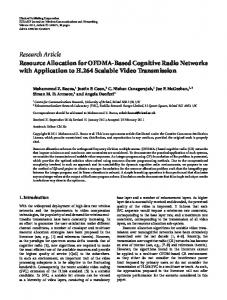
max . Similar to Step Step 2: Next, we prove ω+ m,i ≤ 10I 1, if i is allocated (am,i = 1), the claim is straightforward. Now suppose i is not allocated (am,i = 0). Let node k be the allocated node closest to i. We divide the whole plane into 5 fan-like areas as shown in Fig. 8, where ∠1 = 120◦ with node k in its middle, and ∠2 = ∠3 = ∠4 = ∠5 = 60◦ . For each area, we find the allocated node closest to i (Fig. 8). An important property of the selected nodes is that in each area, any allocated node will generate more interference to the selected node than to i. Define set Ψ to be the collection of these nodes. Clearly |Ψ| ≤ 5. Let T = { j| j ∈ / Ψ ∧ am, j = 1} be the set of allocated nodes not in Ψ. By geometry, any node in T generates more interference to some node in Ψ than to i. Formally,

∀ j ∈ T , ∃q ∈ Ψ s.t. I j,q ≥ I j,i . + The above I j,q ≥ I j,i also implies I + j,q ≥ I j,i from definition. Consequently,

∑ I +j,i ≤ ∑ ∑ I +j,q ≤ ∑ ω+m,q ≤ 5I max .

j∈T

q∈Ψ j∈T

q∈Ψ

max and |Ψ| ≤ 5. The last inequality holds from ω+ m,q ≤ I Therefore, we have reached the conclusion in Step 2: + + max +5I max = 10I max . ω+ m,i = ∑ j∈Ψ I j,i + ∑ j∈T I j,i ≤ 5I