164
IEEE TRANSACTIONS ON COMMUNICATIONS, VOL. 60, NO. 1, JANUARY 2012
Spectrum Sensing Algorithms via Finite Random Matrices Wensheng Zhang, Student Member, IEEE, Giuseppe Abreu, Senior Member, IEEE, Mamiko Inamori, Member, IEEE, and Yukitoshi Sanada, Member, IEEE
Abstract—We address the Primary User (PU) detection (spectrum sensing) problem, relevant to cognitive radio, from a finite random matrix theoretical (RMT) perspective. Specifically, we employ recently-derived closed-form and exact expressions for the distribution of the standard condition number (SCN) of uncorrelated and semi-correlated random dual central Wishart matrices of finite sizes in the design Hypothesis-Testing algorithms to detect the presence of PU signals. In particular, two algorithms are designed, with basis on the SCN distribution in the absence (ℋ0 ) and in the presence (ℋ1 ) of PU signals, respectively. Due to an inherent property of the SCN’s, the ℋ0 test requires no estimation of SNR or any other information on the PU signal, while the ℋ1 test requires SNR only. Further attractive advantages of the new techniques are: 𝑎) due to the accuracy of the finite SCN distributions, superior performance is achieved under a finite number of samples, compared to asymptotic RMT-based alternatives; 𝑏) since expressions to model the SCN statistics both in the absence and presence of PU signal are used, the statistics of the spectrum sensing problem in question is completely characterized; and 𝑐) as a consequence of 𝑎) and 𝑏), accurate and simple analytical expressions for the receiver operating characteristic (ROC) – both in terms of the probability of detection as a function of the probability of false alarm (𝑃D versus 𝑃F ) and in terms of the probability of acquisition as a function of the probability of miss detection (𝑃A versus 𝑃M ) – are yielded. It is also shown that the proposed finite RMT-based algorithms outperform all similar alternatives currently known in the literature, at a substantially lower complexity. In the process, several new results on the distributions of eigenvalues and SCNs of random Wishart Matrices are offered, including a closed-form of the Marchenko-Pastur’s Cumulative Density Function (CDF) and extensions of the latter, as well as variations of asymptotic the distributions of extreme eigenvalues (Tracy-Widom) and their ratio (Tracy-Widom-Curtiss), which are simpler than those obtained with the “spiked population model”. Index Terms—Spectrum sensing, random matrix, standard condition number, cognitive radio, hypothesis test.
I. I NTRODUCTION
T
HE ability to reliably detect the presence/absence of an unknown (possibly weak) signal emitted by a Primary User (PU) amidst additive white Gaussian noise (AWGN) is Paper approved by R. M. Buehrer, the Editor for Cognitive Radio and UWB of the IEEE Communications Society. Manuscript received November 19, 2010; revised July 8, 2011 and September 13, 2011. Parts of this work were presented at the Asilomar Conference on Signals Systems and Computers, 2010, and the Int. Conf. on Comm. (ICC), 2011. W. Zhang, M. Inamori, and Y. Sanada are with the Dept. of Elect. and Electrical Eng., Keio University, 3-14-1 Hiyoshi, Kohoku, Yokohama, 223-8522 Japan (e-mail:
[email protected], {inamori, sanada}@elec.keio.ac.jp). G. Abreu is with the School of Engineering and Science, Jacobs University Bremen gGmbH, Campus Ring 1, 28759 Bremen, Germany (e-mail:
[email protected]). Digital Object Identifier 10.1109/TCOMM.2011.112311.100721
fundamental to enable efficient autonomous (cognitive) utilization of spectrum by multiple radios. This problem, referred to as spectrum sensing is therefore of major importance in the field of wireless communications and at the core of the cognitive radio paradigm [1]–[3]. It has been recently shown that spectrum sensing algorithms of superior performance and robustness can be designed using the eigenvalues of Wishart random matrices constructed from channel samples [4]–[7]. In [4], for instance, spectrum sensing methods were proposed which rely on the property that the eingenvalues of 𝐾 × 𝑁 Wishart random matrices, with (𝐾, 𝑁 ) → ∞ and a constant aspect ratio 𝜌 ≜ 𝑁/𝐾, follow the Marchenko-Pastur (MP) law [8]. The MP law establishes that the largest (𝜆𝐾 ) and smallest (𝜆1 ) eigenvalues of large matrices converge – under very mild assumptions on the statistics of entries themselves – to constants (𝜆U and 𝜆L ), determined solely by 𝜌 and the signal and noise powers. Using this property, two Hypothesis Testing (HT) spectrum sensing methods, one based on the comparison of 𝜆𝐾 against 𝜆U , and the other based on the comparison of the standard condition number (SCN) 𝜆𝐾 /𝜆1 to the ratio 𝜆U /𝜆L , were designed. A characteristic of random matrix theoretical (RMT) methods based on SCN’s is that no estimate of noise or signal power is required (blindness), which is attractive in crowded spectrum scenarios where background interference aggregate into AWGN [9] with power dependent on the number of active users. A major limitation of approaches based on the deterministic MP model, however, is that the converge-rate 1 [10] of the MP law – which is of order 𝒪(𝐾 − 2 ) – is not fast enough. To improve on this limitation, an RMTbased spectrum sensing method employing a statistical SCN model was proposed [5], in which the Tracy-Widom (TW) distribution [11], [12] is used to model the random nominator, while the MP law is maintained for the constant denominator, leading to an approximate SCN distribution used to relate the test-threshold 𝛾 to a prescribed probability of false alarm 𝛼. Intuitively, the TW-based method of [5] should be superior to that of [4] under a smaller number of samples, since the random nature of SCN’s of finite matrices is accounted for and the rate of convergence of the TW law [13] – which is of order 2 𝒪(𝐾 − 3 ) – is faster than that of the MP law. However, a direct comparison of the MP and TW approaches, which though not provided in [5] is given here in Fig. 1(a), reveals that the TW method outperforms the MP alternative only at large SNR’s. This is because the SCN is truly a ratio of two variates, such that the approximation implicit in the normalization of 𝜆𝐾 by
c 2012 IEEE 0090-6778/12$31.00 ⃝
ZHANG et al.: SPECTRUM SENSING ALGORITHMS VIA FINITE RANDOM MATRICES
𝜆L , as done in [5], is not sufficiently accurate unless 𝜆𝐾 is sufficiently large (which occurs at larger SNR’s). This issue was improved upon in [6], [7], where Curtiss formula on the distribution of the ratio of random variates due to [14] was combined with a recent result on the distribution of the smallest [15] and largest [16], [17] eigenvalues of Wishart random matrices, leading to a more accurate model for their SCN’s for the case when PU signal is present [18]. Indeed it can be seen from Fig. 1(a) that the latter method – which we dub Trace-Widom-Curtiss (TWC) – outperforms the former two across a wide SNR range. However, the TW distribution [11], [19] and the Curtiss formula [14] are highly involved functions which are hard to evaluate numerically and intractable in mathematical analysis. Adding to (and in spite of) this complexity drawback is the fact that all aforementioned statistical models are asymptotic and thus, only approximately applicable to finite and small numbers of samples. This rationale calls for a new approach that requires less samples than current RMT-based spectrum sensing methods. This article addresses the spectrum sensing problem from a finite RMT perspective. In particular, we invoke recent results on the exact distribution of standard condition numbers of dual Wishart random matrices in order to design algorithms that require only a few samples and outperform all the RMT techniques currently known. Notice that if the number of samples available is small, the utilization of dual Wishart matrix models does not constitute a limitation1 , since SCN’s are computed only form the largest and smallest eigenvalues, and since for a given number 𝑀 of samples, a choice of 𝐾 > 2 would also imply a choice for a smaller 𝑁 (see Section II-A), which in turn leads to worse performance (see Section IV). The remainder of the article is as follows. In Section II, we revise relevant asymptotic models for the eigen-properties (eigenvalues, extreme eigenvalues and standard condition number) of random Wishart matrices and spectrum sensing algorithms utilizing such models. Several new results are also offered, including: a closed form expression for the Marchenko-Pastur CDF (Lemma 1); the corresponding asymptotic distributions of the eigenvalues of Wishart matrices constructed from noisy samples of a random (Corollary 2) and constant (Lemma 2 and Corollary 3) PU signal; and slightly simplified asymptotic expressions for the PDFs and/or CDFs of SNC’s of Wishart matrices based on the Tracy-WidomCurtiss formulas (Corollaries 5 and 6, Lemma 4 and Corollary 7). In Section III, the recently discovered finite model for the SCN of Wishart matrices is introduced. The corresponding blind and semi-blind spectrum sensing algorithms are briefly described and compared against equivalent asymptotic-RMT methods in Section IV. The relationship between the false alarm and miss-detection probabilities is also established, based on which it is shown that blind spectrum sensing is supe1 It has been recently shown [20], [21] in the blind case (no receiver ∑ knowledge of PU signal or noise statistics) the test-statistic 𝜆𝐾 / 𝑘 𝜆𝑘 , associated with the Generalized Likelihood Ratio Test, is asymptotically optimum. This article, however, is concerned with spectrum sensing methods with a finite and small number of samples. It can be shown that under such conditions the GLRT-based test is not optimum.
165
rior to semi-blind approach at low SNR’s, and only marginally worse in the high SNR regime. Concluding remarks are finally offered in Section V II. A SYMPTOTIC E IGENSPECTRUM AND SCN M ODELS A. Receive Sample Model Consider the standard AWGN model for an 𝑖-th sample of baseband received signal √ (1) ℎ𝑖 = 𝛽 ⋅ 𝑠𝑖 + 𝑛 𝑖 where 𝛽 is the SNR, 𝑠𝑖 is the PU signal2 including the effect of the channel, 𝑛𝑖 are i.i.d. variates such that 𝑛𝑖 ∼ 𝒩ℂ (0, 1) in which 𝒩ℂ (0, 1) denotes the circularly symmetric complex standard normal distribution and the notation 𝑥 ∼ 𝑝(𝑥) indicates that “𝑝(𝑥)” is the distribution of “𝑥”. Hereafter, 𝑠𝑖 may be either an unknown arbitrary complex constant with ∣𝑠∣ = 1, which models the case when a single symbol of the PU over an AWGN channel is observed, or i.i.d. variates 𝑠𝑖 ∼ 𝒩ℂ (0, 1), which models the case when the PU signal is sampled subject to uncorrelated (fast) Rayleigh fading, and/or is modulated within the received block of samples. It will prove convenient to define now the three hypothesis: ∙ ℋ0 : 𝑠 = 0, (no Primary User signal present); c ∙ ℋ1 : 𝑠 ∕= 0, (constant Primary User signal present); r ∙ ℋ1 : 𝑠 ∕= 0, (random Primary User signal present). Following the model described by equation (1), if a number 𝑀 = 𝐾 × 𝑁 of samples is available, the receiver may build either of the following 𝐾 × 𝑁 random matrices ⎧ H𝑛 if ℋ0 is true (2a) 1 ⎨ H= √ 𝐾 ⎩ √ 𝛽 ⋅ H𝑠 + H𝑛 if ℋ1 is true (2b) In the sequel we summarize several models for the eigenspectrum and SCN’s of Wishart matrices W ≜ H ⋅ H† – where † denotes transpose-conjugate (Hermitian) – with H given either as (2a) or (2b). For clarity, we denote the corresponding probability density functions (PDF’s) and cumulative distribution functions (CDF’s) by 𝑝 and 𝑃 under ℋ0 , ℋ1c and ℋ1r , respectively. Finally, without loss of generality3, all results to follow are for 𝐾 ≤ 𝑁 such that W is full-rank. B. Asymptotic Models for the Eigenspectrum Distribution 1) Under ℋ0 - The Marchenko-Pastur Model: The Marchenko-Pastur law [8], which models the asymptotic eigenspectrum of W under ℋ0 , can be concisely stated as follows. Theorem 1 (Marchenko-Pastur PDF): Let 𝜆∣ℋ0 denote any eigenvalue of W, with H as in equation (2a). Then, √ −𝑟2 + 2(1 + 𝜌)𝑟 − (1 − 𝜌)2 , lim 𝜆∣ℋ0 ∼ 𝑝MP (𝑟; 𝜌) ≜ (𝐾,𝑁 )→∞ 2𝜋⋅𝑟⋅𝐾 𝑁/𝐾=𝜌>1 (3) 2 For simplicity, we follow current literature (𝑒.𝑔. [2], [4], [5]) and focus on a single-PU analysis. However, the technique to be described is general under ℋ0 and can be extended to multi-channel scenarios under ℋ1 . 3 This avoids the unnecessary notational care to handle null eigenvalues.
166
IEEE TRANSACTIONS ON COMMUNICATIONS, VOL. 60, NO. 1, JANUARY 2012
√ √ with 0 < (1 − 𝜌)2 < 𝑟 < (1 + 𝜌)2 . Proof : Due to Marchenko and Pastur, provided in [22]. Implicit within Theorem 1 is the fact that 𝜆 is lower √ bounded by 𝜆L ≜ (1 − 𝜌)2 and upper bounded by 𝜆U ≜ √ 2 (1 + 𝜌) . The Marchenko-Pastur law is known to converge at the rate 𝒪(𝐾 −1/2 ) [10], which is sufficiently fast to enable accurate results to be derived in some problems involving finite random matrices of moderate to large sizes [8]. Hereafter we shall use the term MP-variate to refer to a variate following the Marchenko-Pastur Law. Notice also that, to the best of our knowledge, the Marchenko-Pastur CDF is not available in current literature. Thus, the following result is in order. Lemma 1 (Marchenko-Pastur CDF): ∫𝑟 𝑃MP (𝑟; 𝜌) ≜ 𝜆L
𝑝MP (𝑥; 𝜌)d𝑥 = 12 +𝑝MP (𝑟; 𝜌) + (
(1−𝜌) 2𝜋 asin
(1−𝜌)2 1+𝜌 √ √ 2 𝜌 − 2𝑟 𝜌
)
(4)
) ( 1+𝜌 𝑟 √ − √ + (1+𝜌) asin 2𝜋 2 𝜌 2 𝜌 .
Proof : Let 𝑅 ≜ −𝑟2 + 2(1 + 𝜌)𝑟 − (1 − 𝜌)2 . Then, it is clear from (3) that the integral in equation (4) relates to [23, Eq. 2.267.1] ∫ ∫ ∫ √ √ 𝑏 d𝑟 𝑅 d𝑟 √ , (5) √ + d𝑟 = 𝑅 + 𝑎 𝐹 (𝑟) ≜ 𝑟 2 𝑟 𝑅 𝑅 2
where 𝑎 = −(1 − 𝜌) < 0 and 𝑏 = 2(1 + 𝜌) > 0. The integrals on the righthand-side of equation (5) have closed-form solutions found in [23, Eq. 2.266 and Eq. 2.261], respectively, which yield ∫ ) ( 2 d𝑟 √ √ = (1 − 𝜌)⋅asin (1+𝜌)𝑟−(1−𝜌) 𝐼1 (𝑟; 𝜌) ≜ 𝑎 , (6) 2𝑟 𝜌 𝑟 𝑅 𝐼2 (𝑟; 𝜌) ≜
𝑏 2
∫
) ( d𝑟 √ √ = −(1 + 𝜌)⋅asin 2(1+𝜌)−2𝑟 . 4 𝜌 𝑅
(7)
Thus, from equations (3), (5), (6) and (7) we obtain ) ( 2 √ − (8) 𝐹 (𝑟) = 𝑝MP (𝑟; 𝜌) + (1 − 𝜌)⋅asin (1+𝜌)𝑟−(1−𝜌) 2𝑟 𝜌 ( ) √ (1 + 𝜌)⋅asin 2(1+𝜌)−2𝑟 . 4 𝜌 1 2𝜋 𝐹 (𝑟)
−
1 2𝜋 𝐹 (𝜆L ).
(9)
Finally, notice that 𝑝MP (𝜆L ; 𝜌) = 0, 𝐼1 (𝜆L ; 𝜌) = −𝜋/2 and 𝐼2 (𝜆L ; 𝜌) = 𝜋/2, such that equation (9) reduces to equation (4) after some algebra. 2) Under ℋ1 - The Scaled and Extended Marchenko-Pastur Models: The eigenspectrum distributions of W under ℋ1 differs depending on whether the PU signal is random or constant. In the first case, the following result applies. Corollary 1 (Scaled Marchenko-Pastur PDF): Let 𝜆∣ℋr denote any eigenvalue of W, with H as in 1 equation (2b) and H𝑠 ∼ 𝒩ℂ𝐾×𝑁 (0, 1). Then, lim 𝜆∣
r (𝐾,𝑁 )→∞ ℋ1 𝑁/𝐾=𝜌>1
∼ 𝑝(𝑠) (𝑟; 𝜌, 𝛽) ≜ MP
∫𝑟
(𝑠)
𝑃MP (𝑟; 𝜌, 𝛽) ≜
𝑝(𝑠) (𝑥; 𝜌, 𝛽)d𝑥 = MP
1 ⋅𝑝 (𝑟/(1 + 𝛽); 𝜌). (10) 1 + 𝛽 MP
1 2𝜋 𝐹
(
𝑟 1+𝛽
)
+ 12 . (11)
0
Proof : The result follows immediately from Lemmas 1 and Corollary 1. The distribution of 𝜆∣ℋr with a constant PU signal is 1 governed by the following result. Lemma 2 (Extended Marchenko-Pastur PDF): Let 𝜆∣ℋc denote any eigenvalue of W, with H as in 1 equation (2b) and H𝑠 = 𝑠 ⋅ 1𝐾×𝑁 , where 1𝐾×𝑁 is a matrix whose elements are all 1’s, while 𝑠 is an unknown complex constant with ∣𝑠∣ = 1. Then, lim
(𝐾,𝑁 )→∞ 𝑁/𝐾=𝜌>1
𝜆∣ℋc ∼ 𝑝(𝑒) (𝑟; 𝜌, 𝛽) ≜ MP
(12)
1
lim
(𝐾,𝑁 )→∞ 𝑁/𝐾=𝜌>1
𝐾−1 𝛿(𝑟 − 𝑁 ⋅ 𝛽) 𝑝MP (𝑟; 𝜌) + , 𝐾 𝐾
where 𝛿(𝑟) is the Dirac delta function and 𝛽 > 0. Proof : Start with the Law of Large numbers [24] which √ yields, 1 under a√ constant H𝑠 and a zero-mean H𝑛 , W = 𝐾 ( 𝛽 ⋅H𝑠 + 1 H𝑛 ) ⋅ ( 𝛽 ⋅ H𝑠 + H𝑛 )† = 𝐾 (𝛽 ⋅ H𝑠 ⋅ H†𝑠 + H𝑛 ⋅ H†𝑛 ). 𝛽 Obviously the matrix 𝐾 ⋅ H𝑠 ⋅ H†𝑠 has a single non-zero eigenvalue given by 𝑁 ⋅ 𝛽, while the eigenvalues of the matrix 1 ⋅ H𝑛 ⋅ H†𝑛 are MP-variates. W𝑛 ≜ 𝐾 For convenience, let us denote the 𝑘-th largest eigenvalues of W and W𝑛 respectively by 𝜆𝑘 (W) and 𝜆𝑘 (W𝑛 ), such that 0 < 𝜆1 (W) ≤ 𝜆1 (W) ≤ ⋅ ⋅ ⋅ ≤ 𝜆𝐾 (W) and likewise 0 < 𝜆1 (W𝑛 ) ≤ 𝜆1 (W𝑛 ) ≤ ⋅ ⋅ ⋅ ≤ 𝜆𝐾 (W𝑛 ). Next, invoke the refined Wenyl bounds recently derived in [25, Eq. (2.3)], which yield 𝜆𝑘 (W𝑛 ) ≤ 𝜆𝑘 (W) ≤ 𝜆𝑘+1 (W𝑛 ),
It follows that the Marchenko-Pastur CDF is given by 𝑃MP (𝑟; 𝜌) =
Proof : Since H𝑛 ∼ 𝒩ℂ𝐾×𝑁 (0, 1), if H𝑠 ∼ 𝒩ℂ𝐾×𝑁 (0, 1) then H ∼ 𝒩ℂ𝐾×𝑁 (0, 1 + 𝛽). Consequently 𝜆∣ℋr behaves as (1 + 1 𝛽) ⋅ 𝜆∣ℋ0 . In other words, 𝜆∣ℋr is equivalent to a scaled MP1 variate, with scaling coefficient (1 + 𝛽), which immediately yields equation (10). The distribution 𝑝(𝑠) (𝑟; 𝜌, 𝛽), which is clearly suitable to MP Rayleigh fading case, will be henceforth referred to as the type-0 model for 𝜆∣ℋr . 1 Corollary 2 (Scaled Marchenko-Pastur CDF):
∀ 1 ≤ 𝑘 ≤ 𝐾 −1. (13)
The latter bound indicates that the 𝑘-th eigenvalue of W is “trapped” between the 𝑘-th and 𝑘 + 1-th eigenvalues of W𝑛 , with probability 1 as 𝐾 → ∞. But it has also been recently shown [26] that the mean gap between consecutive eigenvalues of √ large 𝐾 × 𝐾 random Hermitian matrices is given by 1/ 𝐾, and consequently the implication of inequality (13) is that the distribution of the set of eigenvalues {𝜆1 (W), ⋅ ⋅ ⋅ , 𝜆𝐾−1 (W)} converges in probability to the distribution of the set {𝜆1 (W𝑛 ), ⋅ ⋅ ⋅ , 𝜆𝐾 (W𝑛 )}, which is 𝑝𝜆 (𝑟; 𝜌), as per Theorem 1. It is left to show that the asymptotic distribution of 𝜆𝐾 (W) converges in probability to 𝛿(𝑟−𝑁 ⋅𝛽)/𝐾. To this end, invoke the recent result on the distribution of spiked eigenvalues [27], from which the expected value of 𝜆𝐾 is given by E[𝜆𝐾 (W)] =
1 𝑁 ⋅𝛽 (𝑁
⋅ 𝛽 + 1)2 −→ 𝑁 ⋅ 𝛽. 𝑁 ≫1/𝛽
(14)
ZHANG et al.: SPECTRUM SENSING ALGORITHMS VIA FINITE RANDOM MATRICES
Consequently, lim 𝜆𝐾 (W) → 𝑁 ⋅ 𝛽,
𝐾→∞
(15)
which means that the distribution of 𝜆𝐾 (W) is 𝛿(𝑟−𝑁 ⋅𝛽)/𝐾, concluding the proof. Interpreting Lemma 2 requires care. First, as clarified in the Lemma’s statement, the result requires that SNR is strictly non-zero. Otherwise we are obviously in the case discussed in Subsection II-B1. And secondly, the Lemma establishes that for any 𝛽 > 0, the largest eigenvalue of W converges, with probability 1, to 𝜆𝐾 = 𝑁 ⋅ 𝛽 → ∞ as the dimension 𝐾 of W grows unboundedly. What matters, however, is that in that the distributions of 𝜆∣ℋ1 differ substantially depending on whether the PU signal is random or constant. In particular, in the latter case, Lemma 2 implies that there exists a pair critical values of 𝛽 below which the “constant” eigenvalue located at 𝑛 ⋅ 𝛽 falls inside the range (𝜆L , 𝜆U ). Consequently, it can be expected that the√presence of (1 − 𝜌)2 ≤𝛽≤ a constant PU signal with SNR in the range 𝑁 √ 2 (1 + 𝜌) cannot be identified with basis on the eigenvalues 𝑁 of W. For completeness, let us conclude this subsection with the following corollary. Corollary 3 (Extended Marchenko-Pastur CDF): ∫𝑟
(𝑒)
𝑃MP (𝑟; 𝜌, 𝛽)
≜
𝑝(𝑒) (𝑥; 𝜌, 𝛽)d𝑥 MP
0
=
lim
(𝐾,𝑁 )→∞ 𝑁/𝐾=𝜌>1
(16)
167
2) Under ℋ1 - The Scaled and Extended Tracy-Widom Models: In this subsection we shall follow similar steps to those of the preceding subsection and give a summary of the asymptotic extreme value models for W originated from sample matrices H constructed in the presence of PU signal, as defined in equation (2b). Corollary 4 (Scaled Tracy-Widom PDF and CDF): Consider the centralized and normalized extreme eigenvalues of W ≜ H ⋅ H† with H as in equation (2b) and H𝑠 ∼ ¯ 𝐾 ∣ r ≜ 𝜆𝐾 −(1+𝛽)𝜆U and 𝒩ℂ𝐾×𝑁 (0, 1), which are defined as 𝜆 ℋ (1+𝛽)𝜈 1 ¯1 ∣ r ≜ 𝜆1 −(1+𝛽)𝜆L , where 𝜇 and 𝜈 are as given in Theorem 𝜆 ℋ (1+𝛽)𝜇 1 2. Then ¯ r ∼ 𝑝 (𝑟) ≜ d𝑃TW (𝑟) . (19) lim 𝜆∣ TW (𝐾,𝑁 )→∞ ℋ1 d𝑟 𝑁/𝐾=𝜌>1 Proof : The result is an immediate consequence of Corollary 1 and Theorem 2. Lemma 3 (Extended Tracy-Widom PDF and CDF): Let 𝜆𝐾 ∣ℋc denote the largest eigenvalue of W ≜ H⋅H† , with 1 H as in equation (2b) and a constant H𝑠 = 𝑠 ⋅ 1𝐾×𝑁 , where 1𝐾×𝑁 is a matrix whose elements are all 1’s, while 𝑠 is an unknown complex constant with ∣𝑠∣ = 1. Consider also the centralized and normalized smallest eigenvalue of W defined ¯1 ∣ c ≜ 𝜆1 −𝜆L , where 𝜇 is as given in Theorem 2. by 𝜆 ℋ1 𝜇 Then lim 𝜆𝐾 ∣ℋc ∼
(𝐾,𝑁 )→∞ 𝑁/𝐾=𝜌>1
𝐾 −1 𝑢(𝑟 − 𝑁 ⋅ 𝛽) 𝑃MP (𝑟; 𝜌) + , 𝐾 𝐾
1
𝛿(𝑟 − 𝑁 ⋅ 𝛽) , 𝐾
¯ 1 ∣ c ∼ 𝑝 (𝑟) ≜ d𝑃TW (𝑟) . lim 𝜆 TW ℋ1 d𝑟
(𝐾,𝑁 )→∞ 𝑁/𝐾=𝜌>1
(20) (21)
where 𝑢(𝑟) is the unitary step function. Proof : The result is an immediate consequence of Lemma 2.
Proof : The result is an immediate consequence of Lemma 2 and Theorem 2.
C. Asymptotic Extreme-value Models for the Eigenspectrum Distribution
D. Asymptotic Models for the Distribution of Standard Condition Numbers
1) Under ℋ0 - The Tracy-Widom Model: Theorem 2 (Tracy-Widom PDF and CDF): Consider the centralized and normalized extreme eigenvalues of W ≜ H⋅H† , with H as in equation (2a), which are defined 4 √ √ 𝐾) 3 𝜆𝐾 −𝜆U ¯ 1 ∣ ≜ 𝜆1 −𝜆L , 𝜈 ≜ ( 𝑁 +√ and 𝜆 and 6 ℋ 𝜈 𝜇 0 𝐾⋅ 𝐾𝑁 4 √ √ 𝑁 − 𝐾) 3 ¯ √ 𝜇 ≜ − ( 𝐾⋅ . For conciseness, let 𝜆∣ 6 ℋ0 denote either 𝐾𝑁 4 ¯ ¯ 𝜆𝐾 ∣ℋ0 or 𝜆1 ∣ℋ0 . Then
¯𝐾 ∣ ≜ as 𝜆 ℋ0
d𝑃TW (𝑟) ¯ , lim 𝜆∣ ∼ 𝑝TW (𝑟) ≜ ℋ0 d𝑟 ( ∫ ∞ ) 𝑃TW (𝑟) ≜ exp − (𝑥 − 𝑟)𝑞 2 (𝑥)d𝑥 , (𝐾,𝑁 )→∞ 𝑁/𝐾=𝜌>1
(17) (18)
𝑟
where 𝑞 2 (𝑥) is the Hastings-McLeod solution of the Painlevé equation of type II [11], [19]. Proof : Given in [12] for the largest, and [15] for the smallest eigenvalues, respectively. 4 For real Wishart matrices, a similar result holds, where 𝑃 (𝑟) ≜ TW ∫ ) ( ∫ ) ( exp − 12 𝑟∞ 𝑞(𝑥)d𝑥 exp − 𝑟∞ (𝑥 − 𝑟)𝑞 2 (𝑥)d𝑥 .
It has been recently noted [6] that an asymptotic model for the SCN’s of complex Wishart matrices can be constructed with basis on the results of Theorem 2 and a general result on the distribution of the ratio of random variates due to Curtiss [14]. In this subsection we shall revise the results of [6] in light of the distinct extreme-value distributions yielded under ℋ1r and ℋ1c . Before we proceed, let us point out that while the parameters 𝐾 and 𝑁 are, rigorously speaking ∞ since the results to follow are all asymptotic, the expressions to be given are typically evaluated for finite (large) matrices. Consequently, for the sake of clarity and coherence we shall commit a slight abuse of notation by maintaining 𝐾 and 𝑁 , when application, in the formulas. 1) Under ℋ0 - The Tracy-Widom-Curtiss Model: Theorem 3 (Tracy-Widom-Curtiss PDF): Let 𝜉𝐾 ∣ℋ0 denote the SCN of W ≜ H ⋅ H† , with H constructed in the absence PU signals as indicated by equation (2a). Denote the largest and smallest eigenvalues of W by 𝜆𝐾 ∣ℋ0 and 𝜆1 ∣ℋ0 respectively, and the SCN by 𝜉𝐾 ∣ℋ0 ≜
168
IEEE TRANSACTIONS ON COMMUNICATIONS, VOL. 60, NO. 1, JANUARY 2012
𝜆𝐾 ∣ℋ 𝜆1 ∣ℋ
0
. Then
0
(22) 𝜉𝐾 ∣ℋ0 ∼ 𝑝TWC (𝑟; 𝜇, 𝜈, 𝜆𝐿 , 𝜆𝑈 ) ≜ ∞ ( ( ) ) ∫ 𝑟⋅𝑥 − 𝜆𝑈 𝑥 − 𝜆𝐿 −1 𝑥⋅𝑝TW ⋅𝑝TW d𝑥, 𝜇⋅𝜈 𝜈 𝜇 0
where 𝑝TW (𝑟) is as in equation (19), 𝑖.𝑒., obtained by derivation of equation (17)). Proof : The result follows from [14, Eq. (3.2)]. For Hypothesis Testing purposes the CDF is desirable, the following result is thus in order. Corollary 5 (Tracy-Widom-Curtiss CDF): (23) 𝑃TWC (𝑟; 𝜇, 𝜈, 𝜆𝐿 , 𝜆𝑈 ) = ( ) ∫ ∞ 𝑟 ⋅ (𝜆𝐿 − 𝜇 ⋅ 𝑥) − 𝜆𝑈 𝑝 (−𝑥)⋅𝑃TW d𝑥. 𝜆𝐿 TW 𝜈 𝜇
Proof : By definition (integration) of equation (22) we obtain, after interchanging the order of integration and rearranging (24) 𝑃TWC (𝑟; 𝜇, 𝜈, 𝜆𝐿 , 𝜆𝑈 ) = ⎡ ⎤ ( ) ∫𝑟 ) ∫∞ ( 𝑥 − 𝜆𝐿 ⎣ 𝑦 ⋅𝑥 − 𝜆𝑈 −1 𝑥 ⋅𝑝 𝑝TW ⋅ ⋅ d𝑦 ⎦ d𝑥. 𝜇 𝜇 𝜈 TW 𝜈 −∞
0
𝑈 ≜ 𝑧, the Under the change of variables 𝑦 → 𝑦⋅𝑥−𝜆 𝜈 𝑟⋅𝑥−𝜆 𝑈 ∫ 𝜈 integral within 𝑝TW (𝑧) d𝑧 = ( ) brackets reduces to −∞ 𝑈 Substituting this result into equation (24) yields 𝑃TW 𝑟⋅𝑥−𝜆 𝜈
𝑃TWC (𝑟; 𝜇, 𝜈, 𝜆𝐿 , 𝜆𝑈 ) = (25) ( ) ) ∫∞ ( 𝑥 − 𝜆𝐿 𝑟 ⋅ 𝑥 − 𝜆𝑈 −1 𝑝TW ⋅𝑃TW d𝑥. 𝜇 𝜇 𝜈 0
𝐿 Through another change of variables 𝑥−𝜆 −𝜇 → 𝑤 and under the fact that 𝜇 < 0, we finally arrive at equation (23). 2) Under ℋ1 - The Scaled and Extended Tracy-WidomCurtiss Models: Corollary 6 (Scaled Tracy-Widom-Curtiss PDF and CDF):
Let 𝜉𝐾 ∣ℋr denote the SCN of W ≜ H ⋅ H† , with H 1 constructed in the presence of random PU signals as shown in equation (2b) with H𝑠 ∼ 𝒩ℂ𝐾×𝑁 (0, 1). Denote the largest and smallest eigenvalues of W in this case by 𝜆𝐾 ∣ℋr and 𝜆1 ∣ℋr respectively, such that 𝜉𝐾 ∣ℋr ≜ 1
1
𝜆𝐾 ∣ℋr
1
𝜆1 ∣ℋr
1
. Then
1
SNR 𝜌 be sufficiently high such that5 𝜆𝐾 ∣ℋc > 1 + 1 Then,
√ 𝜌−1 .
𝜉𝐾 ∣ℋ𝑐 ∼ 𝑝(𝑒) (𝑟; 𝜇 ˜ , 𝜈˜, 𝜅, 𝜏 ) ≜ (26) TWC 1 ) ( ∞ √ ( ) ∫ (˜ 𝜇 −𝑥)𝑁 2/3 (𝑟⋅𝑥−𝜅) 𝑁 𝑁 7/6 ⋅ 𝑝TW 𝑥⋅𝑝Gauss d𝑥, 𝜏 𝜈˜ 𝜏 𝜈˜ 0
(𝑟) is standard Normal distribution and 𝜇 ˜ ≜ where 𝑝 √ √ √ Gauss2 √ 4/3 ( ) ( 𝑁 − 𝐾−1) ( 𝑁 − 𝐾−1) 𝛽+1 −1/2 √ √ 𝛽 + 𝜌 , 𝜈 ˜ ≜ , 𝜅 ≜ 6 𝐾 𝛽 𝑁⋅ 𝐾−1 √ 1 𝛽+1 −2 6 2 and 𝜏 ≜ 𝛽 𝛽 −𝜌 . Proof : The standard normality of the scaled and normalized largest eigenvalue of Wishart matrices constructed as indicated in the statement of the Lemma was established in [17], [28]. Specifically, it was shown thereby, with basis on the spiked population model of [27], that under the condition 𝜆𝐾 ∣ℋc > 1 √ 1 1/2 −1 1 + 𝜌 , lim (𝐾,𝑁 )→∞ ⋅ (𝜆𝐾 ∣ℋc − 𝜅)𝑁 ∼ 𝒩 (0, 1). 1 𝑁/𝐾=𝜌>1 𝜏 Likewise, it has been shown in [11], [15] that 1 lim (𝐾,𝑁 )→∞ ⋅ (˜ 𝜇 − 𝜆1 ∣ℋc )𝑁 2/3 ∼ 𝑝TW (𝑟). 1 𝑁/𝐾=𝜌>1 𝜈 ˜ The result in equation (26) then follows by applying Curtiss formula [14, Eq. (3.2)]. Corollary 7 (Extended Tracy-Widom-Curtiss CDF): (𝑒) 𝑃TWC (𝑟; 𝜅, 𝜏,˜ 𝜇,˜ 𝜈) = ( ∫∞ 1 ( ⋅ 𝑟⋅(˜ 𝜇+ 𝑝TW (−𝑥)⋅𝑄 𝜏
(27) 𝜈 ˜ 𝑥) 𝑁 2/3
−𝜅
)√
) 𝑁
d𝑥,
−𝑁 2/3 ⋅˜ 𝜇 𝜈 ˜
where 𝑄 is the Gaussian 𝑄-function. Proof : The result follows directly by integration of equation (26) from Lemma 4, with steps similar to those of the proof of Corollary 5. E. Summary and Comments on Asymptotic-RMT Spectrum Sensing Algorithms In this subsection we summarize relevant results on asymptotic random matrices and briefly discuss their application to spectrum sensing. For convenience, the results of Subsections II-B and II-C are gathered in Table I. The table also allows a quick identification of the new contributions made thereby. Specifically, the closed-form expression of the Marchenko-Pastur CDF given in Lemma 1; and the corresponding scaled variation given in Corollary 2 are new.
𝜉𝐾 ∣ℋr ∼ 𝑝TWC (𝑟; 𝜇, 𝜈, 𝜆𝐿 , 𝜆𝑈 ) and its CDF is the same as in 1 equation (23). Proof : First under the same arguments of those in Corollary 1, we define 𝜆𝐾 ∣ℋr ≜ (1 + 𝛽)𝜆U and 𝜆1 ∣ℋr ≜ (1 + 𝛽)𝜆L . 1 1 Then, since the scaling coefficients (1 + 𝛽) cancel out, the √ 5 In [7, Eq.(61) and (62)] distributions of (𝑟𝑥 − 𝜅) 𝑁 /𝜏 for the cases √ results follow immediately from Theorem 3 and Corollary 5. −1 when 𝜆𝐾 ≤ 1 + 𝜌 are also given, which if replaced for 𝑝Gauss (𝑟) Lemma 4 (Extended Tracy-Widom-Curtiss PDF (high SNR)): would immediately lead to corresponding alternative distributions of 𝜉𝐾 ∣ c ℋ 1
Let 𝜉𝐾 ∣ℋc ≜ 1
𝜆𝐾 ∣ℋc
1
𝜆1 ∣ℋc
1
denote the SCN of W ≜ H ⋅ H†
constructed in the presence of a constant PU signal, that is, with H as in equation (2b) and a H𝑠 = 𝑠 ⋅ 1𝐾×𝑁 , where 1𝐾×𝑁 is a matrix whose elements are all 1’s, while 𝑠 is an unknown complex constant with ∣𝑠∣ = 1. Furthermore, let the
in the same form of equation (26). In the context of our article, however, these are unnecessary since it will be ultimately shown that the finite random matrices models introduced in Section III are superior to the asymptotic ones discussed here. 6 In general, 𝜇 ˜ and 𝜈˜ can √ √ 4/3 ( 𝑁 − 𝐾−𝑈 ) √ √ , where 𝑈 𝑁⋅ 6 𝐾−𝑈
be defined as 𝜇 ˜ ≜
(
√
𝑁−
√
𝐾−𝑈 ) 𝐾
2
and 𝜈˜ ≜
denotes the number of PU’s, such that the result can be extended to multiple PU’s.
ZHANG et al.: SPECTRUM SENSING ALGORITHMS VIA FINITE RANDOM MATRICES
169
TABLE I A SYMPTOTIC R ANDOM M ATRIX M ODELS FOR S PECTRUM S ENSING Variable All Eigenvalues: 𝜆
PDF
a b
CDF
Theorem 1
Ext. Eigenvalues: (𝜆𝐾 , 𝜆1 ) SCN: 𝜉𝐾
Lemma 1
PDF a
Corollary 5
PU Signal Constant: ℋ𝑐1
CDF
Corollary 1
Theorem 2 Theorem 3
Corollary 2
PDF a
Lemma 2
Corollary 4 a
Corollary 6
CDF a
Corollary 3
a
Lemma 3 a
Lemma 4
a
Corollary 7
a,b
New result. For high SNR.
So are the density and distribution of the eigenvalues of the sum of a constant and a random Wishart matrix (𝑖.𝑒., the extended MP PDF and CDF) given in Lemma 2 and Corollary 3. Likewise, the simplified expression of the CDF of the SCN of Wishart matrices based on the Tracy-Widom extreme-value distributions and the Curtiss formulas given in Corollary 5 as well as the extended TWC PDF and CDF that model the case when a constant PU signal is present, given respectively in Lemma 4 and Corollary 7, are minor, but novel contributions. The key functions (CDF’s) and parameters (Test Statistic 𝜁 and Threshold 𝛾) required to design Hypothesis Tests for spectrum sensing with basis on the models described above given a prescribed probability of false-alarm 𝛼 or probability of miss-detection 𝛿 are summarized in Table II. The corresponding functions and parameters required to design equivalent spectrum sensing algorithms with basis on the Finite Random Matrix models to be discussed in Section III are also included for conciseness and future reference. The performances of these algorithms are compared in Figs. 1, 2 and 5. All comparisons were evaluated via MonteCarlo simulations assuming a constant complex signal7 and random circular complex AWGN according to the model shown in (2). Leaving aside the proposed method for the time being, it can be seen that amongst the techniques relying on asymptotic random matrix models, the TWC-based algorithms (𝑒.𝑔. [6], [7]) are generally superior to TW-based algorithms (𝑒.𝑔.[5]), which in turn outperform MP-based algorithms (𝑒.𝑔. [4]). The underperformance of the MP-based algorithm results from the inaccuracy of the model with small sample sizes. To illustrate, the Marchenko-Pastur limiting distribution is compared in Fig. 3 against exact equivalents introduced later in Lemma 6. The figure shows that the Marchenko-Pastur model is sufficiently accurate only of the number of samples (𝐾 ×𝑁 ) is in the order of thousands. It must be noticed, however, that the densities and distribution functions given in Theorem 3, Lemma 4 and Corollaries 5 and 7 are hard to evaluate, which is in stark contrast with the simplicity of the classic Marchenko-Pastur models of Subsection II-B. In other words, the improvement achieved by moving from MP-based to TW-based to TWC-based methods comes at the expense of an increase in complexity and a loss of mathematical tractability. Nevertheless, an interesting connection between the MPbased technique proposed in [4, Sec. III-B] and the TWCbased technique using SCN’s as proposed in [6], [7], 7 Results
PU Signal Random: ℋ𝑟1
PU Signal Absent: ℋ0
for the case of random U signals are similar.
is that neither require the knowledge of noise power, although the MP-based method has a fundamental limitation compared to the alternatives as it does not admit a tolerated probability of false alarm to be accommodated in the hypothesis test. This blind feature is highly desirable since in situations where multiple wireless devices share a crowded spectrum, background noise levels vary with the number of users accessing the channel. Unfortunately, this potential advantage is undermined by the fact that all the aforementioned methods require a large number of samples (large matrices), which in turn implies (contradictorily) that an accurate estimate of the average noise power can be obtained directly from the samples, with accuracy proportional to their number [29]. In conclusion, it is reasonable to say that in order to truly exploit the potential of random-matrix-theoretical approaches to blind spectrum sensing, novel techniques requiring a limited number of samples is required. This is the subject of the subsequent section. III. F INITE R ANDOM M ATRICES E IGEN S PECTRUM AND SCN M ODELS A. Finite Models for EigenSpectrum Distribution 1) Under ℋ0 - The Bronk-Shin-Lee Model: The exact distribution of eigenvalues of uncorrelated central Wishart matrix has been presented in [30] and [31]. Lemma 5 (Bronk-Shin-Lee PDF): Let 𝜆∣ℋ0 denote any eigenvalue of W, with H as in equation (2a). Then, 𝜆∣ℋ0 ∼ 𝑝BSL (𝑟; 𝐾, 𝑁 ) ≜
𝐾−1 1 ∑ 𝑘!⋅𝑟 𝑁−𝐾 ⋅𝑒−𝑟 𝑁−𝐾 [𝐿 (𝑟)]2 , (28) 𝐾 𝑘=0 (𝑁 − 𝐾 + 𝑘)! 𝑘
where 𝐿𝑏𝑎 (𝑥) is the Laguerre polynomial of order 𝑎, ( ) 𝑎 ∑ 𝑎 + 𝑏 𝑥𝑙 𝑙 (29) 𝐿𝑏𝑎 (𝑥) = (−1) ⋅ ⋅ . 𝑎−𝑙 𝑙! 𝑙=0
Proof : Found in [30] and [31]. 2) Under ℋ1 - The Scaled Bronk-Shin-Lee and the Alfano et al. Models: Lemma 6 (Scaled Bronk-Shin-Lee PDF): Let 𝜆∣ℋ𝑟 denote any eigenvalue of W, with H as in 1 equation (2b) and H𝑠 ∼ 𝒩ℂ𝐾×𝑁 (0, 𝛽). Then, ) ( 𝑟 1 ⋅ 𝑝 ; 𝐾, 𝑁 . (30) (𝑟; 𝐾, 𝑁, 𝛽) ≜ 𝜆∣ℋ𝑟 ∼ 𝑝(𝑠) BS 1 1 + 𝛽 BSL 1 + 𝛽 Proof: Follows immediately under arguments similar to those in the proof of Corollary 1. Lemma 7 (Extended Alfano PDF):
170
IEEE TRANSACTIONS ON COMMUNICATIONS, VOL. 60, NO. 1, JANUARY 2012
TABLE II S PECTRUM S ENSING A LGORITHMS FROM R ANDOM M ATRIX T HEORY
ℋ1 Test
ℋ0 Test
Method
a b c
Test Statistic
Threshold 𝛾
𝜁
Cumulative Distribution Function 𝑃 (𝑟)
Marchenko Pastur
𝜆𝐾 ∣ℋ0
√ (1+ 𝜌)2 √ (1− 𝜌)2
Tracy Widom
¯𝐾 ∣ 𝜆 ℋ0
⎡ ⎤ √ 𝑃 −1 (1−𝛼) 𝑁 +𝐾+2√𝑁 𝐾 ⎣ ⎦ ⋅ 1+ √ √ TW√ √ 3 𝑁 +𝐾−2 𝑁 𝐾 ( 𝑁+ 𝐾)2 𝑁 𝐾
𝜉𝐾 ∣ℋ0
−1 (1 − 𝛼) 𝑃TWC
𝜉2 ∣ℋ0
𝑃M−1 (1 − 𝛼)
Tracy Widom Curtiss Finite RMT (Proposed) Extended Tracy Widom Curtiss Finite RMT (Proposed)
(𝑒)−1
(𝛿)
(𝑒)−1
(𝛿)
𝜉𝐾 ∣ℋ𝑐
𝑃TWC
𝜉2 ∣ℋ𝑐
𝑃M
1
1
a
) ( 2 (1−𝜌) 1√ +𝜌 (1−𝜌) √ − (𝑟;𝜌)+ asin 𝑃 (𝑟)= 1 +𝑝 MP MP 2 2𝜋 2 𝜌 2𝑟 𝜌 ) ( (1+𝜌) 1√ +𝜌 𝑟 + − √ asin 2𝜋 2 𝜌 2 𝜌
( ∫ ) 𝑃TW (𝑟) = exp − 𝑟∞ (𝑥 − 𝑟)𝑞 2 (𝑥)d𝑥
𝑃 (𝑟) = TWC
∞ ∫ 𝜆𝐿 𝜇
( 𝑝
TW
𝑃M (𝑟) =
(−𝑧)⋅𝑃 TW
𝑟⋅(𝜆𝐿 −𝜇⋅𝑧)−𝜆𝑈 𝜈
𝑆2 (𝑟; 𝑁 ) − 𝑆2 (1; 𝑁 ) 2(𝑁⎛−(1)!(𝑁 − 2)!
∞ ⎜ ∫ 𝑝 (−𝑥)⋅𝑄⎜ 𝑃 (𝑒) (𝑟) = ⎝ TW TWC −𝜇 ˜ 2/3 𝑁 𝜈 ˜
𝑟 ⋅(𝜇+ ˜
) d𝑧
b
) √ ⎞ 𝜈 ˜ 𝑁 𝑥)−𝜅 ⎟ 𝑁 2/3 ⎟ d𝑥 ⎠ 𝜏
𝑃 (𝑒) (𝑟) = Φ(𝑁, 𝜃1 , 𝜃2 )(𝑆4 (𝑟; 𝑁, 𝜃1 , 𝜃2 ) − 𝑆4 (1; 𝑁, 𝜃1 , 𝜃2 )) c M
For conciseness, a slight abuse of notation is committed by omitting the parameters of each distribution See equations (35) through (37) See equations (42) and (43) through (46)
Let 𝜆∣ℋ𝑐 denote any eigenvalue of W, with H as in 1 equation (2b) and a H𝑠 = 𝑠 ⋅ 1𝐾×𝑁 , where 1𝐾×𝑁 is a matrix whose elements are all 1’s, while 𝑠 is an unknown complex constant with ∣𝑠∣ = 1. Then, exp(−𝜙𝐾 ) ⋅ (31) 𝐾 ⋅((𝑁 − 𝐾)!)𝐾 𝐾 exp((𝛽 + 1) ⋅ 𝑟) ∑ ((𝛽 + 1)⋅𝑟)𝑁 −𝐾+𝑘 × ⋅ 𝐾−2 ∏ 𝑟 𝑘=1 𝜙𝑘−1 𝑙! 𝐾 𝑙=0 [ ] 𝐾−1 𝑖−1 ∑ 𝑟 0 𝐹1 (𝑁−𝐾+1, (𝛽 +1)⋅𝜙𝐾 ⋅𝑟) + ⋅𝐶𝑖,𝑘 , −1 ⟨𝑁−𝐾+1⟩𝑖−1 𝐶𝐾,𝑘 𝑖=1
Then, 𝜉2 ∣ℋ0 ∼ 𝑝M (𝑟; 𝑁 ) ≜
𝜆∣ℋ𝑐 ∼ 𝑝A (𝑟; 𝐾, 𝑁, 𝛽, 𝝓) ≜
𝑃M (𝑟; 𝑁 ) =
1
where 𝝓 = {𝜙1 , ⋅ ⋅ ⋅ , 𝜙𝐾 } is the vector of squared singular values vector of H𝑠 in ascending order, 0 𝐹1 (⋅) is the confluent hypergeometric function, the function ⟨𝑥⟩𝑦 ≜ (𝑥+𝑦−1)! (𝑥−1)! , and 𝐶𝑖,𝑗 is the (𝑖, 𝑗)-th cofactor of 𝐾 ×𝐾 matrix A, whose (ℓ, 𝑘)th elements are defined as ⎧ (𝑁 −𝐾 +𝑘+ℓ − 2)! if 1 ≤ ℓ ≤ 𝐾 −1, (32a) ⎨ [𝑁 −𝐾 +1]ℓ−1 𝑎ℓ,𝑘 ≜ 𝐹 (𝑁 −𝐾 +𝑘, 𝑁 −𝐾 +1, 𝜙ℓ) ⎩0 1 if ℓ = 𝐾. (32b) ((𝑁 −𝐾 +𝑘−1)!)−1 Proof : Given in [32].
𝑆2 (𝑟; 𝑁 ) − 𝑆2 (1; 𝑁 ) , 2(𝑁 − 1)!(𝑁 − 2)!
1) Under ℋ0 - Distribution of SCN of Finite Uncorrelated Central Wishart Matrices: New results on the distribution of the SCN of finite complex random Wishart matrices have been recently reported in [33]. Amongst others, the following closed-form expressions for the distribution of the SCN of dual Wishart matrices are of particular relevance here. Theorem 4: PDF and CDF for Uncorrelated Central Wishart Matrix (𝐾 = 2) Let 𝜉2 ∣ℋ0 ≜ 𝜆2 ∣ℋ0 /𝜆1 ∣ℋ0 ≥ 1 denote the SCN of dual uncorrelated central Wishart matrices W, with H as in equation (2a).
(33)
(34)
where 𝑆𝑖 (𝑟; 𝑁 ) ≜ Δ𝑖 (𝑟;𝑁,𝑁−1)−2Δ𝑖(𝑟;𝑁−1,𝑁 )+Δ𝑖 (𝑟;𝑁−2,𝑁+1), (35) with 𝑖 = {1, 2} and ] [𝑁−1 𝑀 (𝑁 −1)! ∑ (𝑀 +1− 𝑛𝑟 )𝑟𝑛 ∏ 𝑛+𝑚 , (36) Δ1 (𝑟; 𝑀, 𝑁 ) ≜ (𝑟+1)2 𝑛=0 (𝑟+1)𝑛 𝑟+1 𝑚=1 ] 𝑀 𝑁−1 1 ∑ 𝑟𝑛 ∏ 𝑛+𝑚 Δ2 (𝑟;𝑀,𝑁 ) ≜ (𝑁 −1)! 𝑀 !− . (37) 𝑟+1 𝑛=0 (𝑟+1)𝑛𝑚=1 𝑟+1 [
Proof : Provided in [33]. 2) Under ℋ1 - Scaled and Extended SCN Distributions: Lemma 8 (Scaled SCN Model): Let 𝜉2 ∣ℋ𝑟 ≜ 𝜆2 ∣ℋ𝑟 /𝜆1 ∣ℋ𝑟 ≥ 1 denote the SCN of dual un1 1 1 correlated central wishart matrices W, with H as in equation (2b) and H𝑠 ∼ 𝒩ℂ𝐾×𝑁 (0, 𝛽). Then, 𝜉2 ∣ℋ𝑟 ∼ 𝑝M (𝑟; 𝑁 ),
(38)
Pr{𝜉2 ∣ℋ𝑟 ≤ 𝑟} = 𝑃M (𝑟; 𝑁 ).
(39)
1
B. Finite Models for SCN Distribution
𝑆1 (𝑟; 𝑁 ) , 2(𝑁 − 1)!(𝑁 − 2)!
1
Proof : Clearly 𝜆𝑘 ∣ℋ𝑟 follows the same distribution of 𝜆𝑘 ∣ℋ0 – 1 which incidentally can be found in [34]–[36] scaled by (1+𝛽). Consequently, 𝜆2 ∣ℋ𝑟 /𝜆1 ∣ℋ𝑟 follows the same distribution of 1 1 𝜆2 ∣ℋ0 /𝜆1 ∣ℋ0 , concluding the proof. Lemma 9 (Non-central and Semi-correlated Wishart Matrices): ˜ = S ˜ ⋅S ˜ † be a non-central Wishart matrix with Let W ˜ ∈ ℂ𝐾×𝑁 , E[W] ˜ = I𝐾 /(𝛽 + 1) and E[W ˜ ⋅ W] ˜ = Ω. S Consider the central semi-correlated complex Wishart matrix W = S ⋅ S† with S ∈ ℂ𝐾×𝑁 and effective covariance 𝛽⋅Ω I𝐾 + . (40) Σ𝐾 = 𝛽 + 1 (𝛽 + 1)𝑁
ZHANG et al.: SPECTRUM SENSING ALGORITHMS VIA FINITE RANDOM MATRICES
171
TABLE III F INITE R ANDOM M ATRIX M ODELS FOR S PECTRUM S ENSING Variable All Eigenvalues: 𝜆 Largest Eigenvalue: 𝜆𝐾 Smallest Eigenvalue: 𝜆1 SCN: 𝜉𝐾 a b
PU Signal Absent: ℋ0 PDF
CDF
Lemma 5 a [34, Eq.17] [36, Eq.6] [35, Eq.38] [34, Eq.9] [35, Eq.38] [35, Eq.47] Theorem 4
PU Signal Random: ℋ𝑟1 PDF
CDF
Lemma 6 a [34, Eq.17] b [36, Eq.6] b [35, Eq.38] [34, Eq.9] [35, Eq.38] b [35, Eq.47] b Theorem 4
b
PU Signal Constant: ℋ𝑐1 PDF
CDF
Lemma 7 a [34, Eq.12] [34, Eq.2] [35, Eq.43] [35, Eq.44] [35, Eq.97] Theorem 5
CDF obtained by numerical integration from the PDF Obtained by scaling from the ℋ0 distribution
Then, the first- and second-order moments of W differ from ˜ only by Ω/𝑁 . those of W Proof : Provided in [37] Lemma 9 presents a way to approximate the complex non-central Wishart matrix with the complex semi-correlated central Wishart matrix. In light of this result, the ℋ1 test can be designed based on the properties of semi-correlated central Wishart matrices. Theorem 5: PDF and CDF for Semi-Correlated Central Wishart Matrix (𝐾 = 2) Let 𝜉2 ∣ℋ𝑐1 ≜ 𝜆2 ∣ℋ𝑐1 /𝜆1 ∣ℋ𝑐1 ≥ 1 denote the SCN of dual semi1/2 1/2 correlated central Wishart matrices W ≜ (Σ2 H)⋅(Σ2 H)† with H as in equation (2a), where Σ2 , given in (40), is the associated correlation matrix and 𝜃1 > 𝜃2 are its corresponding ordered eigenvalues. Then 𝑆3 (𝑟; 𝑁, 𝜃1 , 𝜃2 ) , (41) Φ(𝑁, 𝜃1 , 𝜃2 ) 𝑆4 (𝑟; 𝑁, 𝜃1 , 𝜃2 ) − 𝑆4 (1; 𝑁, 𝜃1 , 𝜃2 ) 𝑃M(𝑒) (𝑟; 𝑁, 𝜃1 , 𝜃2 ) = , (42) Φ(𝑁, 𝜃1 , 𝜃2 ) where (𝜃2 − 𝜃1 ) ⋅ (𝑁 − 1)!(𝑁 − 2)! , (43) Φ(𝑁, 𝜃1 , 𝜃2 ) ≜ (𝜃1 ⋅ 𝜃2 )1−𝑁 and 𝜉2 ∣ℋ𝑐1 ∼ 𝑝(𝑒) (𝑟; 𝑁, 𝜃1 , 𝜃2 ) ≜ M
𝑆𝑖 (𝑟; 𝑁,𝜃1 ,𝜃2 ) ≜ Δ𝑖 (𝑟;𝑁−1,𝑁−1,𝜃1−1,𝜃2−1 )−Δ𝑖 (𝑟;𝑁−2,𝑁,𝜃1−1,𝜃2−1 ) −Δ𝑖 (𝑟;𝑁−1,𝑁 −1,𝜃2−1,𝜃1−1 )+Δ𝑖 (𝑟;𝑁−2,𝑁,𝜃2−1,𝜃1−1 ), (44) with 𝑖 = {3, 4} and (45) Δ3 (𝑟; 𝑀, 𝑁, 𝜃1 , 𝜃2 ) ≜ ] [𝑁 −1 𝑀 𝑛 𝑛 ∏ ∑ (𝑀 + 1 − 𝑟 )⋅(𝜃1 ⋅ 𝑟) (𝑁 −1)! (𝑛+𝑚) , (𝑟 + 𝜃2 )𝑚+2 𝑛=0 (𝜃1 ⋅ 𝑟+𝜃2 )𝑛 𝑚=1 (𝑁 −1)! Δ4 (𝑟; 𝑀, 𝑁, 𝜃1 , 𝜃2 ) ≜ ⋅ (46) 𝜃1𝑁 [ ] 𝑁 −1 𝑀 𝑛 ∑ ∏ (𝜃1 ⋅ 𝑟) 𝑀! 1 − (𝑛+𝑚) . 𝜃2𝑀+1 (𝜃1 ⋅ 𝑟+𝜃2 )𝑀+1 𝑛=0 (𝜃1 ⋅ 𝑟+𝜃2 )𝑛 𝑚=1 Proof : Provided in [33]. The random matrix models discussed in Sections III-A and III-B are summarized in Table III. IV. S PECTRUM S ENSING A LGORITHMS F ROM R ANDOM M ATRIX T HEORY Together, Sections II and III yield a complete characterization of asymptotic and exact models for the eigenspectra and SCN’s of dual Wishart matrices, both in the absence or in the
presence of a PU signal, be it random or deterministic. In this section we describe how these results can be employed to design spectrum sensing algorithms. First, however, let us elaborate on characteristics of each relevant result in light of this objective. First, notice that the close-form CDF expressions of Lemma 5, Lemma 6 and Lemma 7, besides being hard to evaluate, if used to design spectrum-sensing algorithms would inevitably lead to techniques that would fail at medium to low SNR’s. This is because in that range the eigenvalue associated with an eventual PU signal is no longer the largest and therefore is “trapped” in between noise-related eigenvalues, by force of the Wenyl inequality results [25], [26, Eq. (2.3)] invoked in the proof of Lemma 2. Finite random matrix theoretical spectrum sensing algorithms could likewise be designed with basis on the extreme eigenvalue models lised in Table III. Unfortunately, since these expressions are also very hard to evaluate, and by force of the Wenyl inequalities [25], [26, Eq. (2.3)], such approaches would be likewise plagued by the same issues of computational complexity and poor performance at medium to low SNRS observed in the asymptotic RMT-based approaches discussed previously. Furthermore, both eigenspectrum- and extreme eigenvalue-based techniques do not have the blindness advantage of SCN-based alternatives. Consequently, the most interesting approach is to rely on SCN models. Obviously one could in principle employ the Curtiss formula [14] in combination with the extremeeigenvalue models offered in [34]–[36] (see Table III) to obtain such SCN models, but such an approach would clearly lead to cumbersome expressions. Fortunately, Theorems 4 and 5 present exact and relatively simple PDF and CDF expressions for finite random Wishart matrices that can be readily employed in the design of spectrum-sensing algorithms. To these end, the required parameters for a Hypothesis Test method equivalent to those discussed in Subsection II-E are summarized in Table II. For the ℋ0 case, the finite-RMT spectrum sensing algorithm can be concisely described as follows. Given a prescribed 𝛼 and 2 × 𝑁 samples ℎ𝑘𝑛 : 1− Construct H ≜ [ℎ𝑘𝑛 ]𝑘={1,2}×𝑛={1,⋅⋅⋅𝑁 } ; 2− Compute the eigenvalues (𝜆1 , 𝜆2 ) of W ≜ H ⋅ H† ; 3− Evaluate the ratio 𝜉2 ≜ 𝜆2 /𝜆1 ; (0) −1
4− Accept ℋ0 if and only if 𝜉2 ≤ 𝑃M (1 − 𝛼). Likewise, for the ℋ1 case, given a prescribed 𝛿 and 2 × 𝑁 samples ℎ𝑘𝑛 the ℋ1 test can be summarized as 1− Construct H ≜ [ℎ𝑘𝑛 ]𝑘={1,2}×𝑛={1,⋅⋅⋅𝑁 } ;
172
IEEE TRANSACTIONS ON COMMUNICATIONS, VOL. 60, NO. 1, JANUARY 2012
Detection Performance of RMT Spectrum Sensing (α = 0.05, K = 2, N = 10)
1
0.9
0.9
0.8
0.8
Probability of Acquisition: Pr{ζ < γ|H0 }
Probability of Detection: Pr{ζ > γ|H1 }
1
0.7 0.6 0.5 0.4 0.3 0.2 Proposed Tracy-Widom-Curtiss Tracy-Widom Marchenko-Pastur
0.1 0 −10
−8
−6
−4
−2
0 2 SNR(in dB): β
4
RMT Detection Performance for HT H1 (δ = 0.01, K = 2)
6
8
0.7 0.6 0.5 0.4 0.3 0.2 Proposed(N = 10) Proposed(N = 6) TWC(N = 10) TWC(N = 6)
0.1 0 0
10
1
2
3
(a) Performance against SNR
0.8
0.8
Probability of Acquisition: Pr{ζ < γ|H0 }
Probability of Detection: Pr{ζ > γ|H1 }
0.9
0.7 0.6 0.5 0.4 0.3
0.1 0 0
Proposed (N = 10) Proposed (N = 6) Tracy-Widom-Curtis (N = 10) Tracy-Widom-Curtis (N = 6) Tracy-Widom (N = 10) Tracy-Widom (N = 6)
0.1
0.2
6
7 8 9 SNR(in dB): β
10
11
13
14
15
0.7 0.6 0.5 0.4 0.3 0.2 Proposed Proposed TWC (N TWC (N
0.1
0.3 0.4 0.5 0.6 0.7 Tolerated Probability of False Alarm: α
12
RMT Detection Performance for HT H1 (SNR = 2dB, K = 2)
1
0.9
0.2
5
(a) Performance against SNR
Detection Performance of RMT Spectrum Sensing (SNR = 2dB, K = 2)
1
4
0.8
0.9
1
0 0
0.1
0.2
0.3 0.4 0.5 0.6 0.7 Tolerated Probability of Miss Detection: δ
0.8
(N = 10) (N = 6) = 10) = 6)
0.9
1
(b) Performance against 𝛼
(b) Performance against 𝛿
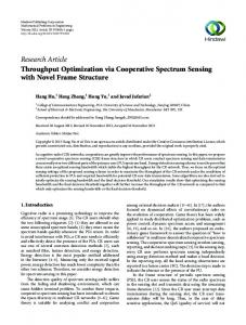
Fig. 1. Probability of detection of spectrum sensing algorithms based on finite random matrix (proposed) and asymptotic random matrix, as a function of the SNR and the tolerated probability of false-alarm.
Fig. 2. Probability of Acquisition of spectrum sensing algorithms based on finite random matrix (proposed), as a function of the SNR and the tolerated probability of false-alarm.
2− Compute the eigenvalues (𝜆1 , 𝜆2 ) of W ≜ H ⋅ H† ; 3− Evaluate the ratio 𝜉2 ≜ 𝜆2 /𝜆1 ; (𝑥) −1
4− Accept ℋ1 if and only if 𝜉2 ≥ 𝑃M (𝛿), where 𝑥 = 𝑠 if the PU signal is random, or 𝑥 = 𝑒 if the PU signal is constant8 . The performances of these algorithms are compared against those of the asymptotic-RMT alternatives in Figs. 1 and 2. First, in Fig. 1(a), the probability of detection of the RMTbased methods over 20 samples are plotted against the signalto-noise-ratio. It is found that the proposed scheme based on Matthatiou et al.’s SCN CDF for finite random Wishart matrices outperforms all the alternatives, exhibiting a 2dB advantage over the asymptotic Tracy-Widom-based method proposed in 8 Notice that in the absence of any knowledge on the PU signal, the assumption of a random signal leads to conservative detection.
[5] – at the “high” SNR region around 0dB – and several dB over the Marchenko-Pastur method at the low SNR region. Notice that the detection probability of all these methods improve(degrade) if either the number of samples or the tolerated probability of false alarm increases(decreases). In order to illustrate this effect, the algorithms are compared in terms of their probability of detection as a function of the tolerated (prescribed) probability of false alarm in Fig. 1(b). The experiments were conducted for an SNR of 2dB. Notice that results for the Marchenko-Pastur method are not shown since this method does not allow for any a priori estimate of the probability of false alarm. It is found not only that the proposed finite RMT-based technique is consistently superior to the alternatives, but also very consistent on its own, in so far as a gradual degradation(improvement) is observed as the tolerated 𝛼 or the
ZHANG et al.: SPECTRUM SENSING ALGORITHMS VIA FINITE RANDOM MATRICES
0.08
173
Scaled Marchenko-Pastur (SMP) Law and Bronk-Shin (SBS) Eigenvalue Distributions
0.07
SCN Distributions of Central Wishart Matrices
0.7
SMP: K → ∞, N → ∞ SBS: K = 20, N = 100 SBS: K = 10, N = 50 SBS: K = 5, N = 25
Theoretical Empirical: 𝐾 = 2, 𝑁 = 10 Empirical: 𝐾 = 2, 𝑁 = 5 Empirical: 𝐾 = 2, 𝑁 = 4
0.6
0.06
𝑝𝜆 (𝑟; 𝐾, 𝑁 )
0.4
0.04
(0)
1
pλ|H(s) (r; N, K, β)
0.5 0.05
0.03
0.3
0.02
0.2
0.01
0.1
0 0
5
10
15
r
20
25
30
0 1
35
(𝑥)
𝛿 = 𝑃M (𝑃M −1 (1 − 𝛼)),
(47)
𝛼 = 1 − 𝑃M (𝑃M
(48)
(𝑥) −1
(𝛿)),
where 𝑥 = 𝑠 if the PU signal is random, or 𝑥 = 𝑒 if the PU signal is constant. These relations can be used to design ℋ0 tests starting from a prescribed probability of miss-detection, as desired in cognitive-radio applications. Plots of 𝛼 as a function of 𝛿 are shown in Fig. 5. For comparison purposes, the relationship evaluated numerically using the asymptotic model is also shown. It can be seen that great discrepancy is observed between the exact (finiteRMT)and the approximate (asymptotic-RMT) approaches, further strengthening the point made in this article. Given these two alternative designs, a question could be asked as to which approach is most effective. To be specific, staring from a prescribed probability of miss-detection, and
5
7
𝑟
9
11
13
15
(a) 𝜉∣ℋ0 , 𝐾 = 2, 𝑁 = 4, 5, 10
Fig. 3. The Marchenko-Pastur asymptotic model for the eigenvalues of random Wishart matrices under ℋ1 with a random PU signal, compared against corresponding exact distributions given in Lemma 6 for a few finite random Wishart matrices.
SCN Distributions of Non-central Wishart Matrices
0.6
Theoretical Empirical: 𝐾 = 2, 𝑁 = 10 Empirical: 𝐾 = 2, 𝑁 = 5 Empirical: 𝐾 = 2, 𝑁 = 4
0.5
0.4 𝑝𝜆 (𝑟; 𝐾, 𝑁, 1, 0.6)
0.3
(1)
number of samples available for decision decrease(increase), while techniques relying on asymptotic RMT results suffer from catastrophic degradation. Results for the ℋ1 test in terms of the probability of acquisition as a function of the SNR are illustrated in Fig. 2(a). It can be seen, for instance, that with an SNR of 4 dB a probability of acquisition of 96% under the constraint that the probability of miss-detection is 𝛿 = 0.05 is achieved with only 20 samples. Only the SNR information of PU signal is needed in the detection, which means the proposed scheme is semi-blind. The superiority of the finite-RMT methods are a direct consequence of the accuracy of the models described by equations (33) and (41), as illustrated in Fig. 4. An additional advantage of the finite-RMT framework is that, since both accurate and simple models for the SCN of finite Wishart matrices exist, it is easy to draw a relationship between the probability of false-alarm 𝛼 and probability of miss-detection 𝛿, namely
3
0.2
0.1
0 1
3
5
7
𝑟
9
11
13
15
(b) 𝜉∣ℋ1 , 𝐾 = 2, 𝑁 = 4, 5, 10 Fig. 4. Probability density function of the SCN of uncorrelated and semicorrelated (𝜃1 = 1, 𝜃2 = 0.6) central dual Wishart random matrices and corresponding empirical distributions of central and non-central dual Wishart random matrices.
under a given SNR, should one employ an ℋ1 test directly, or convert 𝛿 to 𝛼 and employ an ℋ0 instead? In order to answer (partly) this question, we perform the following experiment. Let both 𝛼 and 𝛿 take the same value – say, 3% or 10%. Then, compare the two approaches in terms of the number of samples required to achieve the complementary probabilities of detection 𝑃D and acquisition 𝑃A – that is, 97% or 90%, respectively – as a function of the SNR. The detection performances under the ℋ0 and the ℋ1 tests under such conditions are compared in Fig. 6. It can be seen that, in general, at the low SNR regime the ℋ0 test far is superior than the ℋ1 test. On the other hand, at high SNR’s, the ℋ0 test is only marginally inferior to the ℋ1 test. In other words, this results supports the approach of always (regardless of SNR) converting the tolerated probability of mis-detection 𝛿 into an equivalent probability of false alarm
174
IEEE TRANSACTIONS ON COMMUNICATIONS, VOL. 60, NO. 1, JANUARY 2012
Definite False Alarm based on Miss Detection (SNR = 2dB, K = 2)
1
Proposed (N = 10) Proposed (N = 6) Tracy-Widom-Curtiss (N = 10) Tracy-Widom-Curtiss (N = 6)
0.9 0.8
False Alarm: α
0.7 0.6 0.5 0.4 0.3 0.2 0.1 0 0
0.1
0.2
0.3
0.4 0.5 0.6 Miss Detection: δ
0.7
0.8
0.9
1
Fig. 5. Relationship between the probability of false alarm 𝛼 and the probability of miss-detection 𝛿 under hypothesis tests based on the SCN’s of a finite (dual) random Wishart matrices evaluated from exact and asymptotic (Tracy-Widom-Curtiss) models. 35
Random Matrix Size (K × N, K = 2) on Detection Performance H1 H0 H1 H0
30
Test, Test, Test, Test,
(PA = 0.97, δ = 0.03) (PD = 0.97, α = 0.03) (PA = 0.9, δ = 0.1) (PD = 0.9, α = 0.1)
Similar to previous methods based on asymptotic RMT, the proposed algorithms admits for either a tolerated probability of false alarm 𝛼 or a probability of miss-detection 𝛿 to be accounted for by design. Simple relationships between these two design parameters were also provided. It was shown, however, that the new finite-RMT algorithms not only outperforms known asymptotic-RMT alternatives, but also that the blind approach of employing ℋ0 tests is the best choice overall (optimum at low SNR’s or nearly optimum in the high SNR regime). In addition the above, a comprehensive account of all random matrix-theoretical models relevant for the spectrum sensing applications if given, with several contributions offered, including: a closed-form expression the Marchenko-Pastur CDF (Lemma 1); the scaled variation of the Marchenko-Pastur CDF (Corollary 2 of Lemma 1) that models the asymptotic behavior of the eigenvalues in Wishar Matrices with a constant component; the extended variation of the Marchenko-Pastur PDF (Lemma II-B2) and its CDF (Corollary 3); an explicit (simpler) formula for the Tracy-Widom-Curtiss CDF for the SCN of asymptotically large Wishart matrices in the presence of a distinct random signal (Corollary 5 of Theorem 3); the corresponding scaled version (Corollary 6 of Theorem 3 and 5); the extended Tracy-Widom-Curtiss PDF for the SCN of asymptotically large Wishart matrices constructed in the presence of a distinct constant signal (Lemma 4); and the Corresponding CDF (Corollary 7 of Lemma 4).
Random Matrix Size: N
25
R EFERENCES
20
15
10
5
0 1
2
3
4
5 6 SNR(in dB)
7
8
9
10
Fig. 6. Sample size 𝐾 × 𝑁 required by ℋ1 test and ℋ0 tests, to achieve the same performances as a function of the SNR.
𝛼 and employing ℋ0 , rather than employ the ℋ1 test over 𝛿 directly. This, in turn, further strengthens the relevance of the blind approach advocated in this article. V. C ONCLUSIONS We presented new blind spectrum sensing algorithms based on finite random matrix theory. The algorithm utilizes recently-derived closed-form and exact expressions for the CDF of the SCN of dual random Wishart matrices of finite size, both uncorrelated central and semi-correlated central (which approximates the non-central case). Based on these new models, hypothesis tests are formulated around both the hypothesis ℋ0 that no PU signal is present, and the hypothesis ℋ1 that a PU signal (random or constant) is present .
[1] S. Haykin, “Cognitive radio: brain-empowered wireless communications,” IEEE J. Sel. Areas Commun., vol. 23, no. 2, pp. 201–220, Feb. 2005. [2] T. Yucek and H. Arslan, “A survey of spectrum sensing algorithms for cognitive radio applications,” IEEE Commun. Surveys & Tutorials, vol. 11, no. 1, pp. 116–130, 2009. [3] B. Wang and K. J. R. Liu, “Advances in cognitive radio networks: a survey,” IEEE J. Sel. Topics Signal Process., to be published. [4] L. S. Cardoso, M. Debbah, P. Bianchi, and J. Najim, “Cooperative spectrum sensing using random matrix theory,” in Proc. 2008 IEEE ISWPC. [5] Y. Zeng and Y.-C. Liang, “Eigenvalue-based sectrum sensing algorithms for cognitive radio,” IEEE Trans. Commun., vol. 57, no. 6, pp. 1784– 1793, June 2009. [6] F. Penna, R. Garello, and M. A. Spirito, “Cooperative spectrum sensing based on the limiting eigenvalue ratio distribution in Wishart matrices,” IEEE Commun. Lett., vol. 13, no. 7, pp. 507–509, 2009. [7] F. Penna and R. Garello, “Theoretical performance analysis of eigenvalue-based detection.” Available: http://arxiv.org/abs/0907.1523 [8] A. M. Tulino and S. Verdu, Random Matrix Theory And Wireless Communications, ser. Foundations and Trends in Communications and Information Theory. Now Publishers Inc., 2004. [9] P. C. Pinto and M. Z. Win, “Communication in a Poisson field of interferers—part I: interference distribution and error probability,” IEEE Trans. Wireless Commun., to be published. [10] F. Götze and A. Tikhomirov, “Rate of convergence in probability to the Marchenko-Pastur law,” Bernoulli, vol. 10, pp. 503–548, 2004. [11] C. Tracy and H. Widom, “On orthogonal and sympletic matrix ensembles,” Commun. Mathematical Physics, vol. 177, pp. 727–754, 1996. [12] A. Soshnikov, “A note on universality of the distribution of the largest eigenvalues in certain sample covariance matrices,” J. Statistical Physics, vol. 108, no. 5–6, pp. 1033–1056, 2002. [13] N. E. Karoui, “A rate of convergence result for the largest eigenvalue of complex white Wishart matrices,” Annals Probability, vol. 34, no. 6, pp. 2077–2117, Nov. 2006. [14] J. H. Curtiss, “On the distribution of the quotient of two chance variables,” Annals Mathematical Statistics, vol. 12, no. 4, pp. 409–421, 1941.
ZHANG et al.: SPECTRUM SENSING ALGORITHMS VIA FINITE RANDOM MATRICES
[15] O. N. Feldheim and S. Sodin, “A universality result for the smallest eigenvalues of certain sample covariance matrices,” Geom. Funct. Anal., vol. 20, pp. 88–123, 2010. [16] J. Baik, G. B. Arous, and S. Péché, “Phase transition of the largest eigenvalue for nonnull complex sample covariance matrices,” Annals Probabability, vol. 33, no. 5, pp. 1643–1697, 2005. [17] Z. Bai and J. Yao, “Central limit theorems for eigenvalues in a spiked population model,” Ann. Inst. H. Poincaré Probab. Statist., vol. 44, no. 3, pp. 447–474, 2008. [18] M. Alamgir, M. Faulkner, C. P, and P. Smith, “Modified criterion of hypothesis testing for signal sensing in cognitive radio,” in Proc. 2009 IEEE International Conf. Cognitive Radio Oriented Wireless Networks Commun., pp. 1–4. [19] M. Dieng, “Distribution functions for edge eigenvalues in orthogonal and symplectic ensembles: Painlevé representations,” Ph.D. dissertation, University of California, Davis, 2005. [20] B. Nadler, F. Penna, and R. Garello, “Performance of eigenvalue-based signal detectors with known and unknown noise level,” in Proc. 2011 IEEE International Conference Commun.. [21] P. Bianchi, M. Debbah, M. Maida, and J. Najim, “Performance of statistical tests for single-source detection using random matrix theory,” IEEE Trans. Inf. Theory, vol. 57, no. 4, pp. 2400–2419, Apr. 2011. [22] V. A. Marchenko and L. A. Pastur, “Distributions of eigenvalues for some sets of random matrices,” Math USSR-Sbornik, vol. 1, pp. 457– 483, 1967. [23] I. S. Gradshteyn and I. M. Ryzhik, Table of Integrals, Series, and Products, 6th edition. Academic Press, 2000. [24] A. Papoulis and S. U. Pillai, Probability, Random Variables and Stochastic Processes, 4th edition. McGraw-Hill, 2002. [25] I. C. F. Ipsen and B. Nadler, “Refined perturbation bounds for eigenvalues of Hermitian and non-Hermitian matrices,” SIAM J. Matrix Analysis Applications, vol. 31, no. 1, pp. 40–53, Feb. 2009. [26] T. Tao and V. Vu, “Random matrices: universality of local eigenvalue statistics,” Acta Math. Available: http://arxiv.org/abs/0906.0510 [27] J. Baik and J. W. Silverstein, “Eigenvalues of large sample covariance matrices of spiked population models,” J. Multivariate Analysis, vol. 97, pp. 1382–1408, 2006. [28] D. Féral and S. Péché, “The largest eigenvalues of sample covariance matrices for a spiked population: diagonal case.” Available: http://arxiv. org/abs/0812.2320v1 [29] R. Tandra and A. Sahai, “SNR walls for signal detection,” IEEE J. Sel. Topics Signal Process., pp. 4–17, Feb. 2008. [30] B. V. Bronk, “Exponential ensembles for random matrices,” J. Math Physics, vol. 6, pp. 228–237, 1965. [31] H. Shin and J. H. Lee, “Capacity of multiple-antenna fading channels: spatial fading correlation, double scattering, and keyhole,” IEEE Trans. Inf. Theory, vol. 49, no. 10, pp. 2636–2646, Oct. 2003. [32] G. Alfano, A. Lozano, A. M. Tulino, and S. Verdu, “Mutual information and eigenvalue distribution of MIMO Ricean channels,” in Proc. 2004 Int. Symp. Inf. Theory Applic. [33] M. Matthaiou, M. R. Mckay, P. J. Smith, and J. A. Nossek, “On the condition number distribution of complex Wishart matrices,” vol. 58, no. 6, pp. 1705–1717, 2010. [34] M. Kang and M.-S. Alouini, “Largest eigenvalue of complex Wishart matrices and performance analysis of MIMO MRC systems,” vol. 21, no. 3, pp. 418–426, 2003. [35] A. Zanella, M. Chiani, and M. Win, “On the marginal distribution of the eigenvalues of Wishart matrices,” IEEE Trans. Commun., vol. 57, no. 4, pp. 1050–1060, Apr. 2009. [36] C. G. Khatri, “Distribution of the largest or the smallest characteristic root under null hyperthesis concerning complex multivariate normal populations,” Ann. Math. Stat., vol. 35, pp. 1807–1810, Dec. 1964. [37] W. Y. Tan and R. P. Gupta, “On approximating the non-central Wishart distribution with Wishart distribution,” Commun. Stat. Theory Mehod, vol. 12, pp. 2589–2600, 1983.
175
Wensheng Zhang (S’08) received his M.E. degree in information and systems from Shandong University, Jinan China, in 2005. In 2005, he joined the School of Communication, Shandong Normal University, Jinan, China, as a Lecturer. Since September 2008, he has been a Ph.D. candidate in the School of Integrated Design Engineering, Graduate School of Science and Technology, Keio University, Yokohama, Japan. His research interests focus on cognitive radio and wireless communications. Giuseppe T. F. de Abreu (S’99-M’04-SM’09) received the B.Eng. degree in electrical engineering and a Latu Sensu degree in telecommunications engineering from the Universidade Federal da Bahia (UFBa), Brazil, in 1996 and 1997, respectively. After a brief experience in industry, he joined the Faculty of Engineering of the Yokohama National University, Japan, where he received his M.Eng. and Ph.D degrees in physics and electrical and computer engineering in 2001 and 2004, respectively. In parallel to his graduate studies, he was a Junior Research Scientist at Sony Corporation’s Advanced Telecommunications Laboratory, Tokyo, Japan, from 1999 to 2002, and a Lecturer at Yokohama National University, Yokohama, Japan from 2001 and 2002. Upon obtaining his doctoral degree, he was with the Centre for Wireless Communications at the University of Oulu, Finland, as a Post-doctoral Fellow from 2004 to 2006, and as an Adjunct Professor from 2006 to 2011. In September 2011, he joined the School of Engineering and Sciences of Jacobs University Bremen, Germany, where he is now a Professor of Electrical Engineering and the Chair of Wireless Communications. Prof. Abreu is a leading expert in Europe with extensive experience in pan-European research projects. He holds over a 150 technical publications, which include dozens of journal articles, multiple conference articles, several book chapters and white papers, as well as a few patents. His research interests include communication theory, stochastic geometry and random networks, wireless security, cognitive radio, statistical channel modeling, multi-sensor/antenna signal processing, localization and tracking algorithms, waveform design, space-time coding/decoding, estimation theory, beampattern synthesis, ultra-wideband communications, et al. Mamiko Inamori (S‘08-M‘10) was born in Kagoshima, Japan in 1982. She received her B.E., M.E., and Ph.D degrees in electronics engineering from Keio University, Japan in 2005, 2007, and 2009, respectively. Since October 2009, she has been an assistant professor at Keio University. She received the Young Scientist Award from Ericsson Japan in 2009. Her research interests are mainly concentrated on software defined radio. Yukitoshi Sanada (S’94-M’97) was born in Tokyo in 1969. He received his B.E. degree in electrical engineering from Keio University, Yokohama Japan, in 1992, his M.Sc.degree in electrical engineering from the University of Victoria, B.C., Canada, in 1995, and his Ph.D. degree in electrical engineering from Keio University, Yokohama, Japan, in 1997. In 1997, he joined the Faculty of Engineering, Tokyo Institute of Technology, as a Research Associate. In 2000, he joined the Advanced Telecommunication Laboratory, Sony Computer Science Laboratories, Inc., as an Associate Researcher. In 2001, he joined the Faculty of Science and Engineering, Keio University, where he is now an Professor. He received the Young Investigator Award from IEICE Japan in 1997 and the WPMC Best Paper Award in 2001. His current research interests are in software defined radio, cognitive radio, and OFDM systems.