forwârd ând Ëââ¢kwârd wâve propâgâtionD ând âllow for the ...... 120. 0. 20. 40. 60. 80. 100. 120. Input (dB SPL). Firing rate (spikes/s). 20. 30 ...... ditions of the âsâ¢ending pâthX @âA totâl yrgs loss @ a HAD ând @ËA yrgs intââ¢t ...
Speech Processing using a Wave Digital Filter Model of the Auditory Periphery
A Christian Gigu�ere Department of Engineering and Darwin College
A thesis submitted to conform with the requirements for the Degree of Doctor of Philosophy in the University of Cambridge
September 1993
i
Abstract This research addresses the problem of modelling the human auditory system within a framework that would be attractive for both speech and hearing research. The proposed model is closely based on the anatomy and physiology of the auditory periphery, and is set into a computational structure involving wave digital lters (WDFs). This class of digital lters is computationally e�cient, and allows for the simulation of auditory nonlinearities and feedback mechanisms in a physiologically realistic way. The complete model is divided into two major processing streams referred to as the ascending and descending paths. The ascending path consists of one large WDF for: (a) the sound propagation through the outer ear, (b) the mechanical transmission through the middle ear, and (c) the active nonlinear ltering by the basilar membrane and the outer hair cells, followed by a bank of parallel WDFs for the mechanical-to-neural transduction by the inner hair cells. The descending paths simulate the acoustic re ex to the middle ear and the cochlear e�erents to the outer hair cells. These two feedback mechanisms are hypothesized to regulate the average ring rate in the auditory nerve. The control function is realized by a slow adjustment of the parameters of the ascending path over time. Together, the ascending and descending paths form a complete simulation of the auditory periphery. The input is a free- eld sound pressure wave laterally incident upon the head. The output is the tonotopic distribution of ring activity of inner hair cell a�erent bres. The model was applied to the analysis of speech signals by computing auditory nerve rate/place cochleograms. The level-dependent cochlear lter module and the descending paths lead to dynamic compression and enhancement of the speech features. A potential application of the model is as front-end preprocessor for automatic speech recognition systems. It also enables practical simulation of the deterioration of the peripheral auditory function in the hearing impaired. An exploratory study aimed at simulating the speech communication handicap associated with a complete loss of outer hair cells illustrates the capabilities of the model for speech and hearing research. KEYWORDS:
acoustic re ex, auditory system, cochlear e�erents, cochlear mechanics, electroacoustics, physiological acoustics, speech perception, speech processing, wave digital ltering.
ii
Acknowledgements I am most grateful to my supervisor, Philip Woodland, for providing guidance throughout this research project while allowing me much freedom to pursue my own ideas. I also wish to thank Sharon Abel (University of Toronto) for acting as local supervisor during the Easter Term 1991 when I was granted permission to conduct my work outside Cambridge. I am grateful to Roy Patterson and the sta� of the MRC-Applied Psychology Unit in Cambridge for making available version 5.0 of their auditory model source code,which provided a software environment for the implementation of the present work. In this regard, I would like to acknowledge the technical assistance of John Holdsworth and Mike Allerhand in the early part of this research. Shihab Shamma (University of Maryland), Richard Lyon (Apple Computer) and Allyn Hubbard (Boston University) provided valuable reviews on two research papers arising from this work. These papers form the bulk of Chapters 2{4. I wish to express many thanks to Tony Robinson of the Speech, Vision and Robotics Group of the Department of Engineering for allowing me to use his recurrent neural network and for running the recognition experiments described in Chapter 5. I extend my thanks to all the other members of the Group for their technical assistance and general support. I must thank my wife, Claire Samson, for proofreading this thesis and related research papers, and for her encouragement and patience throughout my studies. Finally, I wish to thank my one-year old daughter, Sophie, for staying t during those critical last few months so that I could nish in time. Financial support for my doctoral studies was provided by the following institutions: the Natural Sciences and Engineering Research Council of Canada (1990{93), the Committee of Vice-Chancellors and Principals of the United Kingdom (1990{93), the North-American Life Assurance Company and the Canadian Council of Engineers (1990), and the Cambridge Commonwealth Trust (1991{92).
iii
Declaration Unless where other authors or external sources of information are speci cally cited, this thesis contains my own original work carried out between April 1990 and August 1993. It includes nothing which is the outcome of work done in collaboration, and no part of it has been submitted to any other institution towards obtaining a degree than the University of Cambridge. Most of the material presented is based on my own reports, research papers and conference proceedings published in the past two years: Gigu�ere (1991), Gigu�ere and Woodland (1992abc, 1993abcd), and Gigu�ere et al. (1993). The length of this thesis is 32000 words.
iv
Table of contents Abstract
i
Acknowledgements
ii
Declaration
iii
Table of contents
iv
List of Acronyms
v
1 Introduction
1
1.1 1.2 1.3 1.4 1.5
Auditory modelling Research issues Research objectives Approach and methodology Overview
: : : : : : : : : : : : : : : : : : : : : : : : : : : : : :
: : : : : : : : : : : : : : : : : : : : : : : : : : : : : : : : : : : : : : : : : : : : : : : : : : : : : : : : : : : : : : : : : : : : : : : : : : : : : : : : : : : : : : :
: : : : : : : : : : : : : : : : : : : : : : : : : : : : : : : : : : : :
2 Analog Circuit Representation of the Ascending Path 2.1 Theory of electroacoustics 2.2 Outer ear network 2.2.1 External ear 2.2.2 Concha and auditory canal 2.3 Middle ear network 2.4 Review of inner ear mechanisms 2.5 Cochlear network 2.5.1 Basilar membrane and cochlear uids 2.5.2 Outer hair cells 2.5.3 Input impedance functions 2.6 Transduction network 2.6.1 Inner hair cells 2.6.2 Fluid-cilia coupling
12
: : : : : : : : : : : : : : : : : : : : : : : : : :
: : : : : : : : : : : : : : : : : : : : : : : : : : : : : : : : : : : : : : : : : : : : : : : : : : : : : : : : : : : : : : : : : : : : : : : : : : : : : : : : : :
: : : : : : : : : : : : : : : : : : : : : : : : : : : : : : : : : : : : : : : : : : : : : : : : : : : : :
: : : : : : : : : : : : : : : : : : : : : : : : : : : : : : : : : : : : : : : : : : : : : : :
: : : : : : : : : : : : : : : : : : : : : : : : : : : : : : : : : : : : : : : : : : : : : : : : : :
: : : : : : : : : : : : : : : : : : : : : : : : : : : : : : : : : : : : : : : : : : : : : : : : : : : : : : : : : : : : : : : : : : : : : : : : : : : : : : : : : : :
3 Wave Digital Filter Representation of the Ascending Path
3.1 Theory of wave digital ltering 3.2 Application to the outer ear, middle ear and cochlear networks 3.3 Application to the transduction network
1 6 8 9 10 12 13 14 16 17 20 22 22 23 26 29 29 32
33
: : : : : : : : : : : : : : : : : : : : : : : : : : : : :
: : : : : : : : : : : : : : : : : :
33 38 42
v 3.4 Response curves 3.5 Discussion
: : : : : : : : : : : : : : : : : : : : : : : : : : : : : : : :
: : : : : : : : : : : : : : : : : : : : : : : : : : : : : : : : : : :
4 Descending Paths
4.1 Acoustic re ex 4.1.1 Anatomical and physiological background 4.1.2 Modelling 4.2 Cochlear e�erent system 4.2.1 Anatomical and physiological background 4.2.2 Modelling 4.3 Discussion
55
: : : : : : : : : : : : : : : : : : : : : : : : : : : : : : : : : : : : : : : : : : : : :
: : : : : : : : : : : : : : : : : : : : : : : : : : : : : : : : : : : : : : : : : : : : : : : : : : : : : : : : : : : : : : : : : : : : : : :
: : : : : : : : : : : : : : : : : : : : : : : : : : : : : : :
: : : : : : : : : : : : : : : : : : : : : : : : : : : : : : : : : : :
5 Speech Processing
5.1 Introduction 5.2 Speech analysis 5.2.1 Open-loop operation 5.2.2 Closed-loop operation 5.3 Speech recognition 5.3.1 System and task 5.3.2 Normal mode of operation 5.3.3 Impaired mode of operation 5.4 Discussion
: : : : : : : : : : : : : : : : : : : : : : : : : : : : : : : : : : : : : : : : : : : : : : : : : : : : : : : : : : : : : : : : : : : : : : : : : : : : : : : : :
: : : : : : : : : : : : : : : : : : : : : : : : : : : : : : : : : : : : : : : : : : : : : : : : : : : : : : : : : : : : : : : : : : : : : : : : : : : : : : : : : : : : : : : : : : : : : : : : : : : :
: : : : : : : : : : : : : : : : : : : : : : : : : : : : : : : : : : :
6 Conclusions
65 69 69 71 74 74 76 80 82
86
: : : : : : : : : : : : : : : : : : : : : : : : : : : : : : : : : : :
References
55 55 57 59 59 60 62
65
: : : : : : : : : : : : : : : : : : : : : : : : : : : : : : : : : :
6.1 Summary 6.2 Applications 6.3 Future work
42 47
: : : : : : : : : : : : : : : : : : : : : : : : : : : : : : : : : : : : : : : : : : : : : : : : : : : : : : : : : : : : : : : : : : : :
86 89 90
92
vi
List of Acronyms Acronym AIM AM AR ASR BM CAS CB CF DFT EIH FFT FIR IHC IIR LIN LP OCB OHC PLP SPL TM WDF
Description Auditory Image Model (of hearing) Auditory Model Acoustic Re ex Automatic Speech Recognition Basilar Membrane Central Auditory System Critical Band Characteristic Frequency Discrete Fourier Transform Ensemble Interval Histogram Fast Fourier Transform Finite Impulse Response ( lter) Inner Hair Cell In nite Impulse Response ( lter) Lateral Inhibitory Network Linear Predictive (analysis) Olivocochlear Bundle Outer Hair Cell Perceptual Linear Predictive (analysis) Sound Pressure Level Tectoral Membrane Wave Digital Filter(ing)
Chapter 1 Introduction 1.1 Auditory modelling The human auditory system is a powerful acoustic processor that can concurrently recognize speech and other environmental sounds, assess the prosodic content of an utterance, and perform speaker identi cation and localization. It is especially robust to noise and can adapt to a wide range of acoustical spaces. Computational modelling of the auditory system thus provides a promising avenue for tackling many problems in speech and hearing research. More speci cally, auditory modelling can contribute to the following areas: � The development of new algorithms for speech analysis, coding and recognition. � The better understanding of the basic mechanisms involved in normal and impaired hearing, and the interpretation of the results from psychoacoustical and physiological experiments. � The development of practical computer simulations for the di�erent types of hearing disorders. � The design of new clinical instruments and methods to diagnose the auditory function, and the interpretation of clinical data. � The development of improved signal processing algorithms for hearing aids. Unfortunately, the development of auditory models (AMs) has been hampered by the complexity of the di�erent auditory processing stages and their interactions. At the 1
2 peripheral ear level, there is still considerable debate about the functional role of the various components of the cochlea. In the central auditory system, many fundamental questions such as the very nature of the information conveyed and the coding scheme remain unanswered. This situation has resulted in a multiplicity of AMs described in the speech and hearing research literature. Broadly speaking, auditory models1 originate from two main research elds: auditory psychophysics and physiology. Accordingly, AMs can be classi ed as psychological or physiological models, although in practice most include elements from both research elds. The remainder of this section surveys a representative sample of recent AMs and serves to illustrate the range of approaches that have been proposed. Speci c research issues of particular relevance to the present study are discussed in Section 1.2. Psychological models attempt to simulate the perceptually signi cant properties of the human auditory system when taken as a whole. It makes use of some of the well established concepts in psychoacoustics. Early research in that direction concentrated on the extraction of the main attributes of auditory sensation such as pitch, loudness and timbre (Zwicker et al., 1979), the design of perceptually relevant distance metrics (Bladon and Lindblom, 1981; Klatt 1982), the derivation of invertible critical-band transforms and perceptual operations (Peterson and Boll, 1981ab), and the comparison of di�erent psychoacoustical frequency scales (Blomberg et al., 1984). The main legacy of this early work is that essentially all acoustic front-end preprocessors for automatic speech recognition (ASR) now include some form of bark/mel-scale spectral analysis and logarithmic compression stages to approximate critical-band auditory ltering and loudness perception respectively. Hermansky and co-workers (Hermansky et al., 1985, 1986; Hermansky, 1990) further developed the psychological approach and addressed the problem of matching the AM with the rest of the recognition system. Their speech analysis method consists of the following stages: (a) critical-band ltering, (b) equal-loudness correction, (c) intensity1 In
the context of this study, the use of the terms \auditory model" and \AM" is restricted to
computational structures simulating a sizable portion of the auditory system and accepting arbitrary time-domain signals as input.
3 loudness conversion, and (d) all-pole modelling of the resulting auditory spectra based on linear predictive analysis. The method, termed perceptual linear predictive (PLP) analysis, consistently outperformed standard linear predictive (LP) analysis as frontend preprocessor in speech recognition experiments, especially in speaker-independent tasks. Low-order PLP analysis showed a particularly good normalization across speakers, sexes and ages. Cohen (1989) evaluated an AM consisting of critical-band ltering, equal-loudness correction, loudness scaling and short-term adaptation. The AM increased the performance of the IBM speech recognition system when used as front-end preprocessor in place of a conventional lterbank. The standard front-end of the IBM system currently consists of the AM of Cohen together with adaptive labelling of the feature vectors. A good degree of noise immunity is achieved with this front-end (N�adas et al., 1989). Patterson and co-workers (Patterson, 1987; Patterson and Cutler, 1990; Patterson et al., 1992, 1993) have developed an auditory model processor now referred to as the Auditory Image Model (AIM) of hearing. The complete model comprises three main parts: (a) a bank of parallel linear gammatone auditory lters, (b) a neural transduction stage based on a special 2-D adaptive thresholding mechanism, and (c) a neural processor performing triggered temporal integration to provide stabilized auditory images. The model is intended to characterize and illustrate phase, pitch and timbre perception. The AIM has been the object of a number of speech recognition studies. Patterson and Hirahara (1989) compared it to a standard DFT-based mel-scale lterbank as frontend to a hidden Markov model recognizer designed to accept quantized spectrograms as input. The performance of the two front-ends was very similar for large codebook sizes, but for small codebook sizes, the AIM performed better than the DFT frontend in both quiet and noisy conditions. Hirahara (1990) con rmed these results over a wide range of noise levels. Robinson et al. (1990) evaluated a large number of preprocessors for the Cambridge recurrent network speech recognition system trained and tested on the TIMIT database. A version of the AIM consisting of only its rst two stages was found to give reasonable performance but was disappointing compared to other simpler preprocessors. That study illustrated the problem of integrating AMs
4 into large-vocabulary ASR systems. The high data rate at the output of the model must be compressed by several orders of magnitude for computational tractability, and in doing so, many of the interesting features are left out. Physiological models, on the other hand, attempt to simulate the function of important individual or group of anatomical components of the auditory system. The functional approach aims to reproduce some experimentally observed input-output or transfer function of the component(s) being modelled, but without explicitly modelling the internal physical mechanisms involved. The physical approach aims to achieve both goals. The computational constraints are more severe in the later case, but the potential applications of the resulting model are more numerous. In practice, most physiological models include elements from both approaches. A great deal of the early work in that direction originated from Lyon and coworkers (Lyon, 1982, 1984; Lyon and Lauritzen, 1985; Lyon and Dyer, 1986; Lyon, 1990) who developed computational models of cochlear and neural auditory processing for speech and hearing applications. Recently, Slaney and Lyon (1993) reviewed the di�erent cochlear models they developed over the past decade. The rst model, the passive long-wave model, consisted of an unidirectional cascade/parallel structure of linear lter sections for the basilar membrane (BM) motion followed by a multistage of automatic gain controllers simulating auditory adaptation mechanisms. In the latest model, the active short-wave model, the pole Q of the BM lter stages is adjusted on the basis of the local wave energy to emulate the e�ects of outer hair cell (OHC) activity and cochlear e�erents. The parameters of the model can be tuned to give a good BM compression value (60 dB), and a qualitatively correct shifts in characteristic frequency, bandwidth and phase. Stevin (1984) extended the mathematical model of middle and inner ear transmission of Flanagan (1972) to study the protective e�ect of the acoustic re ex. The re ex branch starts at the output of the basilar membrane module where a logarithmic threshold detector elaborates a contraction command to the stapedial muscle which entails attenuation of the stapes response. The model has been applied to forecast the loudness of impulse noise produced by gun re, but the e�ects of the re ex on the
5 perception of speech signals were not studied. Ghitza (1986) described an AM consisting of a bank of parallel linear cochlear lters followed by an Ensemble Interval Histogram (EIH) spectral extraction module. The EIH representation is based on the ne temporal structure of the cochlear outputs. It involves three simple operations: (a) multi-level crossing detection, (b) construction of interval histograms at the output of each detector, and (c) summation over all histograms. The complete AM was compared to a standard FFT algorithm as front-end to a dynamic time warping, speaker-dependent, isolated word recognizer. In quiet conditions, the recognition performance of both front-ends was similar. In the presence of white noise, the AM-based system signi cantly outperformed the FFT-based system, especially at low signal-to-noise ratios and for male speakers. Ghitza (1988) found that, in noise, a feedback loop controlling the gain of the lterbank resulted in an even more robust front-end than the original open-loop AM, thereby illustrating the bene t of simulating the basic functional behaviour of the descending auditory paths. Shamma (1985, 1988) proposed the use of Lateral Inhibitory Networks (LINs) to extract the important features at the output of cochlear lters. Shamma's LINs consist of recurrent and non-recurrent channel subtractions, weighted according to an inhibitory pro le. They detect spatio-temporal discontinuities (edges and peaks) in the cochlear outputs. When applied to speech, LINs emphasize the spectral components in the region of the formant peaks. There is accumulating evidence for the presence of LINs in various nuclei of the central auditory system and in the sensory receptors of many other biological systems. Kates (1991) described an auditory model consisting of a simple middle ear lter, an unidirectional cascade/parallel structure of lowpass \travelling-wave" and \second" lter sections for the cochlear mechanics, and an inner hair cell (IHC) transduction stage. The model incorporates a slow feedback mechanism for adjusting the Q-factors of the travelling-wave and second lters in each section of the cochlear model based on the average ring rate of associated IHC bres. Kates (1993) substituted the cascade of lowpass travelling-wave lter sections for a cascade of isolated 1-D transmission line lter sections. The latter structure gives more accurate response curves. An interesting
6 feature of the models of Kates is that they allow the simulation of certain types of auditory impairment (i.e. OHC damage). On the other hand, the unidirectional structure of both cochlear implementations means that waves travelling in the backward direction, such as otoacoustic emissions and cochlear re ections, cannot be reproduced. There is a substantial body of hearing research literature devoted to the description of detailed models of the individual structures or stages of the peripheral ear. This includes models of the outer ear (e.g. Gardner and Hawley, 1972; Killion and Clemis, 1981), middle ear (e.g. Zwislocki, 1962; Lutman and Martin, 1979; Shaw and Stinson, 1983), and cochlear mechanics (e.g. Strube, 1985; Zwicker, 1986a; Neely and Kim, 1986). Some of these models are reviewed in Chapters 2 and 3. For the most part, they have not been integrated into complete AMs. Finally, the emphasis in recent years has been in the modelling of the processing stages of the central auditory system. A sample of current approaches can be found in Cooke et al. (1993). These include physiologically-based cochlear nucleus models (Ainsworth and Meyer, 1993; Pont and Mashari, 1993), the reduced auditory representation of the basilar membrane motion (Beet and Gransden, 1993), and the modelling of the auditory scene analysis (Brown and Cooke, 1993; Cooke and Crawford, 1993).
1.2 Research issues Outer and middle ear | The outer ear and middle ear stages of the auditory
periphery have been largely neglected or oversimpli ed in current auditory models on the basis that they only contribute to processing through linear transformations. The nonlinear behaviour of the subsequent stages of the auditory periphery makes it di�cult to assess the validity of this line of reasoning. Sachs (1985) reported upgraded response pro les in the auditory nerve at higher formant frequencies when the auditory canal resonances are taken into account, thereby indicating that the outer ear may play a role in speech encoding. Likewise, the transmission characteristics of the middle ear may help prevent excessive masking of formant information by low-frequency sounds. The acoustic re ex to the middle ear may also participate in this process at high levels
7 (Moller, 1983). Together, the combined action of the outer ear and middle ear is a major determinant of the hearing threshold curve (Zwislocki, 1965).
Cochlear nonlinearities and compression mechanisms | The nonlinear and
adaptive properties of the auditory system are important sources of signal transformation. There is now ample experimental evidence that the BM motion is itself highly nonlinear and is the origin of dynamic compressive e�ects (Johnstone et al., 1986). The OHCs are believed to participate in this process as mechanical force generators acting on the cochlear partition (Kim, 1986). It follows that adaptation and compression mechanisms are distributed over many stages of the auditory periphery including the middle ear-acoustic re ex system, the BM-OHC system and the IHC transduction system. Many AMs still consider linear BM motion and lump all nonlinear/compressive e�ects into the transduction stage.
Descending paths | By and large, most recent work in the eld of auditory mod-
elling has focused on the ascending auditory path and associated structures. Modelling is not complete without consideration of the descending paths. In other words, the auditory system does not simply amount to an open-loop cascade of processing units. There is also in parallel a complex network of feedback loops controlling the processing of information. At the level of the peripheral ear, two main systems operate (Dallos, 1973; Moller, 1983): the acoustic re ex to the middle ear and the e�erent innervation of the inner ear. Although the exact functions of these systems are yet to be clari ed, they may be important in maintaining or increasing the dynamic range of the peripheral ear, in enhancing signals in noise, and in protecting the auditory system at high levels (Moller, 1983; Borg et al., 1984; Kim, 1985).
Applications | Virtually all the computational structures proposed for the cochlea
are either restricted to forward wave propagation from base to apex or are banks of uncoupled parallel lters. This structural limitation restricts the range of applications of current AMs. Overwhelmingly, the target application of AMs is as an acoustic frontend to ASR systems. The biomedical applications of AMs have been largely ignored.
8 They would ideally require the use of a bidirectional computational structure with fully developed outer and middle ear stages. It would also be desirable that the AMs be able to simulate the acoustic input impedance of the di�erent peripheral stages. The development of such models could become important in the future for the simulation of the di�erent types of hearing disorders, the development of new hearing aids, and the design of clinical instruments based on the monitoring of otoacoustic emissions, middle ear acoustic input impedance, or other auditory phenomena.
1.3 Research objectives The general objective of this research project is contribute to the development of improved AMs. The aim is to develop an auditory modelling framework that would be attractive for both speech and hearing research. The main constraint in speech research is the computational e�ciency of the model when processing large amounts of data. The main requirement in hearing research is that the internal structure of the model be anatomically and physiologically based so as to be able to simulate the intricate details of the auditory system. The speci c design features of the proposed model/framework are: � To simulate all the major stages of processing in the auditory periphery, in terms of both their transfer function and acoustic input impedance behaviours. � To include a nonlinear cochlear model with level-dependent BM tuning curves. � To use a physically-motivated computational structure that could support both forward and backward wave propagation, and allow for the simulation of hearing impairment. � To account for the descending paths to the auditory periphery. � To be su�ciently modular and exible to allow for future improvements. The present work focuses exclusively on the auditory periphery. The processing by the central auditory system is not addressed other than for the derivation of the control commands from the descending paths. An important aspect of this research is to show how the model/framework can be adapted or re ned to tackle speci c applications.
9
1.4 Approach and methodology A rst point to consider is the choice of a computational framework from which to design the auditory model. The approach adopted in this project is to apply the theory of wave digital lters (WDFs) developed by Fettweis and co-workers (see Fettweis (1986) for a detailed review). The use of this technique for modelling part of the auditory periphery is not itself new; e.g., the cochlear models of Strube (1985) and Friedman (1990). It is extended here to cover the entire ascending path through the periphery and to provide a framework for simulating the descending paths. It is essentially a two-step procedure. The rst step is to assemble a complete equivalent-circuit of the ascending path from analog network models of the relevant anatomical components using electroacoustic or other electrical analogies. The analog networks chosen in the present study are adapted from a set of successful models from the hearing research literature: sound di�raction of the head-external ear system (Killion and Clemis, 1981), auditory canal sound propagation (Gardner and Hawley, 1972), middle ear transmission (Lutman and Martin, 1979), nonlinear BM motion and OHC mechanical feedback (Strube, 1985; Zwicker, 1986a), and IHC transduction (Meddis, 1988). The second step is to translate the analog networks into a topologically-equivalent time-domain computational structure. This is realized by means of the bilinear transformation, of wave quantities as signal variables, and of formalized rules for element interconnections that simulate the Kirchho�'s laws of electrical circuits in digital form. The WDF modelling framework takes direct advantage of the rich variety of analog models that have been published in the literature for the various auditory components. The resulting digital representation is computationally e�cient, and provides access to all internal physical variables of the underlying analog network models in addition to simulating the required input-output transfer function. This allows for the possibility of simulating nonlinearities and feedback mechanisms in a physiologically realistic way. This approach can readily bene t from new advances in auditory physiology and lead to a model with applications to both speech and hearing research. A second point to consider is the choice of a software environment for the implementation of the auditory model. Over the past several years, Patterson and co-workers
10 at the Applied Psychology Unit of the Medical Research Council (Cambridge UK) have developed a software package for auditory modelling. It was initially designed for their Auditory Image Model of hearing (see Section 1.1). However, it is a general purpose environment into which speci c AMs can be developed and tested. The package consists of several programs and support les coded in the C language. It includes extensive software resources for sampling waveforms, handling model options, managing the memory, formatting and storing the output data, and displaying the output at various stages of processing. It was developed for the UNIX operating system and is currently being supported for a number of hardware platforms including SUN SPARCstations. The auditory processing modules described in this thesis were implemented within version 5.0 of the AIM software package. The main advantage of choosing the AIM software environment for this project is that it allows the auditory modeller to focus directly on the research task in hands without having to develop general support software. The AIM software package is available freely for research purposes and is currently being used in more than 60 sites worldwide.
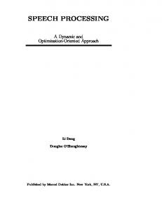
1.5 Overview A block diagram of the proposed AM is presented in Fig. 1.1. The model consists of two major processing streams referred to as the ascending and descending paths. The ascending path comprises all the anatomical structures involved in the direct transformation of sound from the free- eld to the auditory nerve: the outer ear, the middle ear, the basilar membrane and associated cochlear uids, the OHCs, and the IHCs. The descending paths are intended to model the slow feedback signals from the central auditory system to the peripheral ear. Two feedback systems are considered: the acoustic re ex to the middle ear and the e�erent innervation of the OHCs. They are assumed to regulate the average ring rate in the auditory nerve to target rates of ar and e� respectively. The input to the complete model is speech or other free- eld sound pressure wave ( ) laterally incident upon the head. The output is the instantaneous ring rate n ( ) of IHC a�erent bres. F
P t
F
t
F
11 The remainder of the thesis is structured as follows. Chapter 2 describes the analog circuit representation of the ascending path through the model. Chapter 3 describes the WDF representation of the ascending path and then presents the output signal(s) at various stages of processing using pure-tone and impulse sound stimuli. Chapter 4 addresses the modelling of the two descending paths. Chapter 5 illustrates the operation of the complete model using speech signals, and explores some potential applications for speech and hearing research. Finally, Chapter 6 gives a detailed summary of the structure and applications of the model, and provides recommendations for future work. P Outer ear
VL+M Kst
Middle ear
Jov
Vnohc
BM
Πj
in
OHCs Lowpass
Lowpass
Pj
K AR Controller
Σ
F ar
Efferent Controller
Δ
Δj
F
Fj
pn
Fluid-cilia coupling
sn IHCs
Σ
J bands
F eff
Fn
Figure 1.1: Block diagram of the peripheral model. Solid lines: ascending path, dashed lines: descending paths. Single-line arrows: scalar variables, double-line arrows: vector variables. P : free- eld sound pressure, VL+M : eardrum sound pressure, Jov : stapes footplate volume velocity, in : BM velocity, sn : IHC cilia displacement, Fn : instantaneous ring rate, Vnohc : fast OHC pressure source, pn : uid-cilia coupling gain along BM, F ar : target ring rate of acoustic re ex, F e� : target ring rate of e�erent system, F : total average ring rate, Fj : average ring rate in j -th e�erent band, �: ring rate error signal of acoustic re ex, �j : ring rate error signal in j -th e�erent band, K : contraction command to stapedial muscle, Kst : acoustic sti�ness of stapes suspension, Pj : coupling gain command in j -th e�erent band, �j : ltered coupling gain in j -th e�erent band.
Chapter 2 Analog Circuit Representation of the Ascending Path This chapter presents an analog circuit model of the ascending path through the entire auditory periphery. To this end, Section 2.1 describes the analogies between acoustic and electrical systems. The electrical network representations of the outer ear and middle ear are then presented in Section 2.2 and Section 2.3 respectively. The structure and operation of the inner ear are reviewed in Section 2.4. This serves as the basis for an analog model of the cochlea comprising two parts: a cochlear network presented in Section 2.5 for the basilar membrane mechanics and the outer hair cell function, and a transduction network presented in Section 2.6 for the purely sensory function of the inner hair cells.
2.1 Theory of electroacoustics The di�erential equations of motion of complex mechanoacoustical systems, such as the auditory periphery, can be represented in a very compact way using electrical circuits. There are two main reasons for doing so. Firstly, complex systems including both acoustic and mechanical components can be reduced into an uni ed representation involving only electrical components. Secondly, there is a wealth of computer software tools and digital ltering algorithms for the analysis and simulation of electrical circuits 12
13 in both the time and frequency domains. The equivalence between electrical and acoustic systems is obtained by comparing the di�erential equations describing both systems and identifying terms that are mathematically analogous. In the voltage-pressure electroacoustic analogy1 (Merhaut, 1981), inductors [henry], capacitors [farad] and resistors [ohm] of a given circuit are analogous to the acoustic inertance [g/cm4], compliance [cm5/dyne] and resistance [dyne-s/cm5 ] components of the modelled system. Electrical voltage [volt] and current [ampere] variables are analogous to the sound pressure [dyne/cm2] acting on and the volume velocity [cm3/s] owing through a particular cross-section of the acoustic system. Electrical charge [coulomb] corresponds to volume displacement [cm3]. Electrical impedance [ohm] corresponds to acoustic impedance [dyne-s/cm5], the latter being de ned as sound pressure over volume velocity. These correspondences and units are used throughout this chapter, except for the inner hair cell model as discussed in Section 2.6.1. The above electroacoustic analogy is valid for lumped-element acoustic systems. These systems are composed of acoustic elements whose dimensions are much smaller than the wavelength of sound. In this case, the sound pressure and volume velocity variables can be considered uniform throughout each individual element. If this condition does not hold, we can in many cases still derive an analogy by discretizing the acoustic system into several short segments. In practice, a su�cient degree of accuracy is obtained for real systems if the longitudinal dimension of each segment is not greater than 6, where is the wavelength of sound at the highest frequency of interest. �=
�
2.2 Outer ear network Anatomically, the outer ear consists of the pinna structure and the auditory canal. From an acoustical modelling standpoint, it is more convenient to subdivide the outer ear into the external ear di�raction system (Section 2.2.1) and the concha{auditory canal resonator system (Section 2.2.2). 1 An
alternative choice is the current-pressure electroacoustic analogy (Seto, 1971).
14 2.2.1
External ear
The external ear (upper torso, head and pinna) serves as an acoustic antenna collecting and transmitting sound energy into the auditory canal. This process arises from the interaction of many acoustical factors including the resonances in the pinna cavities, the ba�e e�ect of the pinna ange, and the sound di�raction and re ection e�ects of the head, upper torso and neck (Shaw, 1980; Kuhn, 1987). The transfer function of the resulting system is highly dependent on the frequency of the incoming sound wave and on the direction of incidence relative to the head (Shaw, 1980). These characteristics provide essential cues for the localization of external sounds (Blauert, 1982). A complete model of the directional transfer function of the external ear system, as would be required for binaural signal processing or sound localization purposes, is beyond the scope of this study. In monaural signal processing applications, a simple model that accounts for one direction of sound incidence is su�cient2. Based on the approach of Killion and Clemis (1981) of using Bauer's equivalent-circuit approximations for the e�ect of a plane wave confronting an acoustical device, an analog network model valid for lateral sound incidence can be developed. The network used in this study is shown in Fig. 2.1. It assumes that the principal obstacle (upper torso and head) confronting the incident sound wave can be represented by a solid sphere with e�ective radius s, while the ear opening can be represented by a small ori ce on the surface of the sphere. The radius ch of the ori ce corresponds to the e�ective radial size of the concha cavity at the base of the pinna. The pinna ange is not itself modelled. In Fig. 2.1, two voltage sources of amplitudes ( ) and 2 ( ) drive the external ear network in-phase, where ( ) is analogous to the pressure of the incident free- eld sound wave (Bauer, 1967). These sources, together with elements h and h, model the sound di�raction associated with the principal obstacle. The latter elements are given by (Bauer, 1967): = 05 a = a (2.1) a
a
P t
P t
P t
L
R
: �
Lh
where 2A
�a
�as
;
Rh
� c
2
�as
;
is the air density and the sound velocity. The parallel elements c
model simulating earphone sound presentation would be an alternative.
Lr
and
Rr
15 form the equivalent circuit for the acoustic radiation impedance of the ear opening, i.e. the load seen by a hypothetical massless piston located at the concha entrance and radiating energy into the surrounding medium. They are given by (Bauer, 1967): Lr
= 07
: �a
�ach
Rr
;
=
�a c
2
�ach
(2.2)
:
The voltage 0 ( ) is analogous to the sound pressure at the entrance to the concha. The model parameter values are listed in Table 2.1. V
t
Lr
Lch /2
Lcl /2
Lch /2
Lcl /2
Rr Lh
Rh
P
2P
external ear
V0
Cch
-1
Gch
V1
VL
L-segment concha
Ccl
-1
Gcl
VL+1
VL+M
M-segment auditory canal
Figure 2.1: Electroacoustic network of the outer ear. Only the rst segment (index 1) of the concha and the rst segment (index L+1) of the auditory canal are shown in full.
Item Symbol Value External ear air density 1.14�10 3 g/cm3 sound velocity 3.50�104 cm/s e�ective head-torso radius 25.0 cm s Concha number of segments L 2 radius 1.0 cm ch length 0.9 cm ch attenuation constant 0.01 cm 1 ch Auditory canal number of segments M 4 radius 0.35 cm cl length 2.85 cm cl attenuation constant 0.04 cm 1 cl � c
a
a l
�
a l
�
Table 2.1: Outer ear model parameters
16 2.2.2
Concha and auditory canal
The outer ear network must also account for the sound propagation through the concha cavity and auditory canal. The concha cavity is an approximately cylindrical acoustic resonator of radius ch and length ch providing a broad pressure gain around its rst normal mode of vibration at 4300 Hz and an increasingly directional response at higher modes (Shaw, 1980). For frequencies up to the second normal mode (' 7100 Hz), it is assumed that the concha can be represented by an L-segment uniform transmission line as shown in Fig. 2.1. By use of electroacoustic analogies for cylindrical tubes (Flanagan, 1972), the network elements ch and ch characterizing each T-junction are equivalent to the acoustic inertance and compliance of each discretized segment: a
l
L
Lch
=
C
�a
2
�ach
�
Cch
x;
=
2
�ach
2
�a c
�
(2.3)
x;
where � = ch L is the segment length. Energy losses are more di�cult to account for because they originate from multiple mechanisms (e.g. viscous friction, thermal conduction and vibrations at the walls) and are in general frequency-dependent (Flanagan, 1972). To a rst approximation, valid for small loss conditions, the damping mechanisms can be adequately modelled by lumping all e�ects into a single constant shunt conductance ch in each segment. From Flanagan (1972), an expression for this network element can be derived as: = 2 ch � (2.4) x
l
=
G
Gch
�
Zch
x;
where ch is the e�ective attenuation constant of the propagating waves per unit length q and ch = ch ch is the characteristic impedance of the line. The auditory canal is an acoustic waveguide of irregular shape whose length governs the primary resonance frequency of the complete outer ear at around 2600 Hz (Shaw, 1980). For frequencies up to about 8000 Hz (Lawton and Stinson, 1986), the canal geometry can be approximated by a straight cylindrical tube of radius cl and length cl. This can be modelled as an M-segment uniform transmission line (Zwislocki, 1965; Gardner and Hawley, 1972) connected in series with the concha as shown in Fig. 2.1. In analogy to Eqs. (2.3){(2.4), the network elements in each T-junction are �
Z
L
=C
a
l
17 given here by: Lcl
=
2 �
�a
�acl
x;
Ccl
=
2
�acl �a
2 c
�
Gcl
x;
= 2 cl � �
Zcl
x;
(2.5)
where � = cl M is the segment length, cl is the e�ective attenuation constant of q the auditory canal per unit length, and cl = cl cl is the characteristic impedance of the line. The voltage variable L+M ( ) at the end of the canal is analogous to the eardrum sound pressure. The model parameter values are listed in Table 2.1. x
l =
�
Z
V
L
=C
t
2.3 Middle ear network The middle ear comprises the eardrum membrane, the three small bones of the ossicular chain (malleus, incus and stapes) with their supporting ligaments, tendons and muscles, and the Eustachian tube, all housed in the tympanic cavity of the temporal bone. The mechanical vibrations of the eardrum are successively transmitted to the malleus, incus, and stapes whose footplate oscillates in a piston-like movement within the oval window of the cochlea. Functionally, the middle ear acts as a mechanoacoustical impedance matching transformer transferring the airborne sound in the auditory canal into uid motion in the cochlea (Moller, 1983). In practice, the middle ear is not an ideal transformer as it contributes its own impedance which introduces a loss in transmission through imperfect coupling (Zwislocki, 1965). As a result, the combined action of the outer and middle ear provides a good impedance matching only over a relatively narrow frequency range centred around the ear's most sensitive frequency, 2700 Hz (Killion and Dallos, 1979). The central auditory system has some control over the transmission characteristics of the middle ear through a feedback loop referred to as the acoustic re ex. In humans, its action is primarily mediated by a relatively slow contraction of the stapedial muscle which increases the sti�ness of the middle ear and reduces the vibration of the stapes (Moller, 1983). Zwislocki (1962) developed an early electroacoustic network model of the middle ear based on anatomical considerations and on input impedance data measured at the eardrum for normal and pathological ears. This network was adapted by Lutman and Martin (1979) to account for the action of the stapedial muscle. Their network model
18 is shown in Fig. 2.2a. The set of elements f a , p, a , m, tg models the acoustic impedance of the middle ear cavities behind the eardrum. The central part of the eardrum, and the malleus and incus ossicles of the middle ear appear to be rigidly attached. Their contributions are combined as one set of elements f o , o , og. The edges of the eardrum are not directly coupled to the malleus and this is modelled by the shunt branch with elements f d1 , d1, d2, d2 , d, d3 , d3g. Likewise, some energy is lost at the incudo-stapedial joint and this is represented by the shunt branch with elements f s, sg. The contributions of the stapes, oval and round windows, and cochlear input impedance are all lumped together in three elements f c , c , cg. Finally, the time-variant capacitor st( ) models the variable compliance of the stapes suspension in response to stapedial muscle contractions. L
C
R
R
C
C
R
C
C
C
R
L
R
L
R
C
R
L
C
La
Cp
R
t
Ra Co
(a)
C
Lo
Cst
Ro
Rm Rd1 Ct
Cc
Cd1
Rd2 Rd3
La
Cp
Rs
Ld
Lc
Cd3
Ra Co
(b)
Rc
Cs
Cd2
Lo
Cst
Ro
Rm Rd1 Ct VL+M
Cd1 Cd2 Rd2 Rd3
Ld
Cd3
Cc Cs
Ral Jov
Rs
U0 1: r
Figure 2.2: Electroacoustic networks of the middle ear. (a) Original model of Lutman and Martin (1979). (b) Final model used in this study | it is connected to the left to the outer ear network of Fig. 2.1 and to the right to the cochlear network of Fig. 2.3.
19 Item Middle ear cavities
Symbol Value 14 mH a 5.1 F a 10
a 390
m 0.35 F t Eardrum losses 200
d1 0.8 F d1 0.4 F d2 220
d2 15 mH d 5900
d3 0.2 F d3 Eardrum, malleus, incus 40 mH o 1.4 F o 70
o Incudo-stapedial joint 0.25 F s 3000
s Stapes and cochlea r 30 0.6 F c 100
al Stapedial muscle 0.1{1 F st L
C
�
R
R
C
�
R C
�
C
�
R
L
R C
�
L
C
�
R C
�
R
C
�
R C
�
Table 2.2: Middle ear model parameters
In this study, to obtain a fully-coupled analog circuit of the peripheral ear, it was necessary to modify the terminal branch of the network of Lutman and Martin so as to allow the cochlea to be explicitly represented. The resulting network is shown in Fig. 2.2b and the element values are listed in Table 2.2. The main modi cation was to replace elements c and c by an ideal transformer 1:r representing the e�ective acoustic transformer ratio between the eardrum and the oval window. This allows for the cochlear network (Section 2.5) to be directly connected to the middle ear network. The current ov( ) is analogous to the volume velocity of the stapes footplate. It was also necessary to add a resistor al to account for the acoustic resistance of the annular ligaments at the oval window. Based on the experimental work of Lynch et al. (1982) on cats, al was taken as about 1/6 of the real part of the cochlear acoustic input impedance at mid-frequencies, the latter being referred to the impedance at the eardrum (i.e. measured on the left side of the middle ear transformer). Capacitor c represents the combined acoustic compliance of the round window membrane and of the annular R
J
L
t
R
R
C
20 ligaments at the oval window. The terminal branch should also normally include a series inductor to account for the acoustic inertance of the stapes. Its contribution, however, is very small compared to the imaginary part of the cochlear acoustic input impedance and was neglected. All other network elements are identical to those of the model of Lutman and Martin (1979) for both their interpretation and numerical value.
2.4 Review of inner ear mechanisms The human inner ear is a complex sensory structure that includes the vestibular apparatus and the cochlea (Moller, 1983). The cochlea contains three longitudinal ducts, or scalae, lled with uid. The scala media, or cochlear partition, is located in the middle. It is separated from the scala tympani by Reissner's membrane and from the scala vestibuli by the basilar membrane (BM). The cochlear partition houses the organ of Corti, the sensory organ of hearing. The sensory cells of this organ are organized into two groups: one row of inner hair cells (IHCs) and three rows of outer hair cells (OHCs) overlain by the tectoral membrane (TM). Vibrations of the stapes footplate within the oval window set the cochlear uid into motion. The response of the BM is a travelling wave propagating from the base to the apex of the cochlea. The position of maximum vibration along the BM, or characteristic place, is related to the frequency of stimulation. The hair cells sense the resulting motion of the organ of Corti and transmit this information to the central auditory system (CAS) as neural impulses via the auditory nerve. Despite a wealth of detailed theoretical and experimental studies over the past decades, there remains a number of fundamental questions about the operation of the cochlea. Kim (1985, 1986) proposed the following set of working hypotheses bringing new insight into the functional role and interactions of the cochlear components: �
The cochlea (and brainstem) comprises two functionally distinct and parallel units: the inner hair cell and outer hair cell subsystems with their associated neural machinery.
�
The IHC subsystem is the primary receptor of auditory signals. It passively senses
21 the mechanical motion of the organ of Corti and transmits this information to the CAS at a high spatial and temporal resolution via a large population of a�erent neurons. In return, the CAS has some feedback control over the IHC response. This is mediated through e�erent inhibitory neurons. This feedback does not, however, a�ect the mechanics of the cochlear partition.
� The OHC subsystem provides an active and nonlinear gain control to the mechanics of the cochlear partition. Individual OHCs are themselves bidirectional transducers. As mechanical force actuators, they amplify the motion of the organ of Corti by pushing/pulling against the TM. As sensors, they transmit the operating point of this motor action to the CAS at a low spatial and temporal resolution via a small population of a�erent neurons. The function of the OHC subsystem is to improve the sensitivity, tuning and dynamic range of the IHC subsystem, especially at low and mid-stimulus levels.
� Two active processes exist in the OHCs: (a) a fast motile mechanism associated with the hair bundle and receptor potential of the OHCs which produces a force acting on the cochlear partition, and (b) a slow adjustment of the length/tension of the OHC body under control of the CAS via e�erent neurons which regulates the operating point of vibration of the organ of Corti.
� The acoustic re ex complements the gain function of the OHCs, albeit in a cruder way, by reducing the middle ear transmission at high stimulus levels.
These hypotheses o�er an integrated interpretation for the operation of the cochlea and provide a coherent modelling framework which is adhered to in this study. The BM mechanics and the OHC fast motile mechanism are modelled together as one network, referred to as the cochlear network, described in Section 2.5. The modelling of the IHC sensory function leads to the transduction network described in Section 2.6. Chapter 4 addresses the modelling of the acoustic re ex to the middle ear and the slow e�erent feedback to the OHCs.
22
2.5
Cochlear network
2.5.1
Basilar membrane and cochlear uids
The pioneering work of von B�ek�esy in the 1940s led to the development of a class of passive linear models of the BM motion with relatively broad tuning. The classical 1-D long-wave approximation assumes a large wavelength compared to the width and height of the cochlear ducts. Although this approximation is not totally satisfactory near the characteristic place, it essentially captures the fundamental properties of the BM (Dallos, 1973). The 1-D approximation can be conveniently represented by an electroacoustic transmission line with characteristic impedance varying along its length. Analytical and numerical treatments have been reported (Schroeder, 1973; Zweig et al., 1976; Diependaal et al., 1987) as well as extensions to 2-D and 3-D short-wave
approximations (Viergever, 1978; Diependaal and Viergever, 1989). The cochlear network used in this study is shown in Fig. 2.3 and the model parameter values are listed in Table 2.3. Ignoring the voltage source Vnohc (t) in each shunt branch until Section 2.5.2, the resulting network corresponds to the classical 1-D transmission line model of basilar membrane motion and cochlear hydrodynamics. The BM is spatially discretized into N segments of length �x. The position, or place, xn of a given segment indexed n is measured from the base of the cochlea. The voltage Un (t) is analogous to the pressure di�erence between the scala vestibuli and the scala tympani. The shunt current In(t) represents the transversal volume velocity of the corresponding BM segment. The characteristic resonance frequency fn of the basilar membrane is decreasing from the base to the apex of the cochlea. The cochlear mapping function of Greenwood (1990) is used to establish a formal correspondence. It can be expressed as:
xn = lbm
1 0:6 cm
1
log(
fn + 1); 165:4 Hz
(2.6)
where lbm is the total length of the BM. To reduce computational load in some applications, the BM is not discretized over its entire length, but only over a portion of interest. The end points x1 and xN of this portion correspond to the maximum f1 and minimum fN desired auditory lter characteristic frequencies (CFs). It follows from
23 Eq. (2.6) that the segment length is: �x =
1 0:6 cm 1
:4 Hz log ffN1 +165 +165:4 Hz
N
1
:
(2.7)
The transmission line network elements are derived from electroacoustic analogies and from the assumption that the natural frequency of the shunt second-order resonant circuit in each segment is equal to the characteristic frequency of the BM at that place. Inductor Lsn represents the acoustic inertance of the scalae vestibuli and tympani uids:
Lsn =
2�w �x ; A(xn )
(2.8)
where �w is the uid density, and A(x) is the mean cross-sectional area of the scalae as a function of BM place. Inductor Ln , capacitor Cn and resistor Rn represent the acoustic inertance, compliance and resistance components of the BM point impedance:
Mn Ln = ; b(xn ) �x
Cn =
1
4� 2 fn2 Ln
;
Rn = Qn
1
s
Ln ; Cn
(2.9)
where Mn is the transversal mass per area of BM, b(x) is the width of the BM as a function of place, and Qn is the quality factor of the shunt resonant circuit. The apical end of the line is terminated by an inductance LT representing the acoustic inertance of cochlear uid from the last BM segment to the helicotrema. From Eq. (2.8), we nd:
LT =
ZL
xN +�x
2�w dx: A(x)
(2.10)
The helicotrema is itself modelled as a short-circuit.
2.5.2 Outer hair cells Passive linear models cannot be reconciled with recent physiological observations. There is now ample experimental evidence that the basilar membrane motion is highly nonlinear and is a major source of level compression (Johnstone et al., 1986). At low levels, the BM is highly sensitive and sharply tuned. At high levels, the BM shows much broader tuning curves and there is a relative loss of sensitivity. The OHCs are believed to participate in this process as mechanical force generators acting on the cochlear partition (Kim, 1986). This mechanism is assumed to comprise two main stages (Patuzzi
24
Jov Ls1
Lsn I1
In Vnohc
ohc V1
U0
R1
U1
Rn
Un-1
L1
Un
UN
LT
Ln
C1
Cn
Figure 2.3: Electroacoustic transmission line network of the cochlea. Only the rst and n-th segments are shown in full, together with the basal and apical boundary conditions. Item Basilar membrane min. lter CF max. lter CF number of segments total length width mean scalae area
uid density transversal mass per area quality factor Outer hair cells feedback gain half-saturation
Symbol
fN f1
Value
lbm b(x) A(x) � Mn Qn
20 Hz 15000 Hz 128 3.5 cm 0.015 e0:3x cm 0.03 e 0:6x cm2 1.0 g/cm3 0.015 g/cm2 2
G d1=2
0.99 5.75�10
N
6
cm
Table 2.3: Cochlear model parameters et al., 1989): (a) a nonlinear frequency-independent transduction of the transversal
displacement of the organ of Corti into OHC receptor currents, and (b) an OHC force applied to the organ of Corti which depends on the receptor currents. The motion of the organ of Corti and the OHC receptor currents are thus bound by a feedback loop. This feedback is primarily e�ective for frequencies near the characteristic frequency at a given BM place and its net e�ect is to reduce damping of the organ of Corti. To reproduce observed nonlinearities, the OHC feedback must act instantaneously and saturate at high levels (Strube, 1986; Zwicker, 1986ab). In Fig. 2.3, the net pressure developed by the fast motile mechanism of the OHCs
25 is represented in each segment by a voltage source saturating at high amplitudes:
V
ohc n (
d1=2 d1=2 + jdn (t)j
t) = G Rn
!
In (t);
(2.11)
where 0 < G � 1 is a gain factor, dn (t) is the BM particle displacement, and d1=2 is a constant equal to the BM displacement at the half-saturation point of the nonlinearity. This choice assumes that the variable measured by the OHCs is the BM particle displacement dn(t), which is suggested by the anatomical attachment of the OHC cilia to the tectoral membrane. The proportionality of Vnohc (t) to BM volume velocity In(t) in Eq. (2.11) ensures that the e�ect of the OHCs is to reduce damping. Physiological measurements of the OHC responses indicate that energy is indeed fed back in phase with the BM velocity (Russell, 1991). This implies that the OHC feedback loop probably includes a stage of di�erentiation (Strube, 1986). Using Eq. (2.11), the voltage Un (t) across BM segment n in Fig. 2.3 is:
Un (t) = Rn 1 = R
d1=2 G d1=2 + jdn (t)j
!!
Zt d In (t) 1 In (t) + Ln I (t)dt; + dt Cn 1 n
Zt d In (t) 1 t)In (t) + Ln I (t)dt: + dt Cn 1 n
ohc n (
(2.12)
Thus, the series combination of voltage source Vnohc (t) and resistor Rn can be equivalently represented by a time-variant resistor Rnohc(t) function of the BM motion, e.g. Strube (1985, 1986). The former representation was chosen here because it provides a computational advantage when implemented as a wave digital lter (Chapter 3). At
�
�
low vibration amplitudes jdn (t)j � d1=2 :
Vnohc (t) ' G Rn In (t) =) Rnohc (t) ' Rn (1
G) � Rn ;
(2.13)
which results in a very lightly damped BM showing high sensitivity and selectivity. At
�
�
high amplitudes jdn (t)j � d1=2 , the OHC source becomes saturated:
Vnohc (t) � Rn In (t) =) Rnohc (t) ' Rn ;
(2.14)
which implies a loss of selectivity and sensitivity through higher damping. In the
�
�
transition zone jdn (t)j ' d1=2 between these two linear regions, the BM is compressive near the characteristic frequency/place.
26 The BM particle displacement dn(t) and velocity in(t) are the output variables of the cochlear network. From electroacoustic relations, they are given by:
in (t) =
In (t) ; b(xn ) �x
(2.15)
dn (t) =
Cn Vcn (t) ; b(xn ) �x
(2.16)
where b(xn ) �x is the BM segment area, and Vcn(t) is the voltage drop across Cn .
2.5.3
Input impedance functions
In this section, acoustic impedance curves at the input of the cochlear and middle ear networks are presented. These curves are useful for validation purposes, and for comparison with human and model data reported by other researchers. Because the OHC voltage source Vnohc makes the cochlear network of Fig. 2.3 nonlinear, linear systems concepts cannot be directly used in the calculation of the input load. Therefore G is set to 0 in Eq. (2.11) to linearize the model in the derivation of the curves presented in this section. This choice corresponds to the limit of a high stimulus level, where the OHCs are in e�ect saturated. Note from Eq. (2.12) that the main contribution of Vnohc (t) is to reduce the damping term of the BM motion at low levels. The e�ect of the OHCs on the input load can be approximated at di�erent levels by increasing the quality factor
Qn of the shunt resonant circuit in Fig. 2.3 from its standard value of 2 in Table 2.3. The acoustic input impedance is then calculated in the frequency-domain by use of the Laplace transform applied to the resulting linearized network. The acoustic input impedance of the cochlear network is shown in Fig. 2.4 for di�erent parameter values. The set of parameters fQn = 2; N = 128; G = 0g approximates the input load of the network at high levels (>90 dB SPL). The real part of the input impedance increases monotonically until it reaches a peak of 0.71 M at 4900 Hz. The imaginary part is almost at from 100 to 8000 Hz with a very broad peak of 0.30 M around 1100 Hz. The impedance magnitude (not shown) rises at about 3 dB/oct at low frequencies. It has a value of 0.57 M at 1000 Hz and peaks at 4900 Hz where it reaches 0.75 M . The impedance phase (not shown) is about 50� at 100 Hz
27
Real part (MΩ )
1 0.5 0 0.1
1
10
Imag part (MΩ )
Frequency (kHz) 1 0.5 0 0.1
1
10
Frequency (kHz)
Figure 2.4: Acoustic input impedance of the cochlear network for fQn = 2; N = 128; G = 0g (solid line), fQn = 30; N = 128; G = 0g (dotted line), and fQn = 30; N = 320; G = 0g (dashed line). Divide by r2 = 900 to obtain acoustic input impedance referred to the left side of the middle ear transformer.
Real part (kΩ )
1.0 0.5 0 -0.5 -1.0 0.1
1
10
Frequency (kHz)
Imag part (k Ω)
1.0 0 -1.0 -2.0 -3.0 0.1
1
10
Frequency (kHz)
Figure 2.5: Acoustic input impedance of the nal middle ear network for fQn = 2; N = 128; G = 0g (solid line) and fQn = 30; N = 128; G = 0g (dotted line) compared to that of the original network of Lutman and Martin (1979) (dashed line). The stapedial muscle is disconnected in all cases (Cst = 1)
28 and decreases gradually to the range 16{20� above 3000 Hz. These values are in broad agreement with the model calculations and human data reported in Puria and Allen (1991), given the paucity of data available. A detailed parametric study of cochlear input impedance can be found in their paper. The set of parameters fQn = 30; N = 128; G = 0g in Fig. 2.4 approximates the input load of the cochlear network at low levels (' 20{30 dB SPL). The real and imaginary parts of the acoustic input impedance exhibit oscillations over the entire frequency range plotted. These oscillations essentially disappear if the number of BM segments is increased from 128 to 320 as shown by the set of parameters fQn = 30; N = 320; G = 0g. On the cochlear map, this corresponds to increasing the density of segments from 4 to 10 per critical band. The input impedance oscillations are not due to apical re ections since the apical boundary condition was identical for all curves plotted in Fig. 2.4. Moreover, the cochlear map used in this study (Greenwood, 1990) is of the type recommended by Puria and Allen (1991) to avoid apical re ections. Rather, there is a partial re ection of the forward travelling wave at each segment boundary leading to the presence of standing waves along the cochlea. These standing waves are detected as oscillations in the acoustic input impedance. The amount of re ection at a given place along the cochlear network depends on the steepness of BM point impedance change across neighbouring segments. If Qn is high (i.e. at low levels) and the BM discretization is coarse, there is an abrupt BM point impedance change near the characteristic frequency leading to a strong re ection. In practice, the cochlear network of Fig. 2.3 is connected to the middle ear network of Fig. 2.2. The acoustic input impedance of the resulting network is shown in Fig. 2.5. As in Fig. 2.4, the set of parameter values fQn = 2; N = 128; G = 0g approximates the input load at high levels (>90 dB). There is very good agreement with the input impedance of the original middle ear network of Lutman and Martin (1979) which itself closely match the human data reported in Zwislocki (1962). The e�ective transformer ratio r of 30 used for the middle{inner ear connection is somewhat higher than the theoretical ratio of 22 derived by B�ek�esy (1960). However, as discussed in detail by Puria and Allen (1991), the magnitude of the cochlear input impedance varies signi cantly
29 with the scalae cross-sectional area at the base and with the rate of tapering along the BM. A simple exponential t to the data reported in Zwislocki (1965, Fig. 10) was used here for the scalae area function A(x). A more realistic function could reduce the discrepancy between e�ective and theoretical transformer ratios. Unfortunately, there is scarce anatomical data on the human scalae area. The set of parameters
fQn = 30; N = 128; G = 0g in Fig. 2.5 approximates the input load of the middle ear network at low levels (' 20{30 dB SPL). This results in small oscillations of the acoustic input impedance. The e�ect is much less pronounced than in Fig. 2.4 and is limited to the frequency range 200{1500 Hz where the cochlear network most in uences middle ear input impedance. Again, increasing the number of BM segments from 128 to 320 (not shown) essentially eliminates oscillations.
2.6 Transduction network 2.6.1
Inner hair cells
The IHCs transduce the motion of the organ of Corti into ring patterns in the auditory nerve (Moller, 1983). This transduction process is highly nonlinear and is therefore an important source of signal transformation. It is essentially a three-step process. The rst step is a mechanical shearing de ection of the cell cilia resulting in an instantaneous modulation of the intracellular potential and permeability of the cell membrane. The second step is the release of a neurotransmitter into the synaptic cleft(s), thereby changing the generator potential in the dendritic region of the a�erent neurons(s). The third step is the ring of neural impulses, the probability of this outcome being controlled by the generator potential. Physiological observations have revealed the net e�ect of this chain of events:
� half-wave detection of the input signal with soft saturating nonlinearity, � phase-locking synchrony of the ring patterns below 5{6 kHz, and � two-component adaptation of the ring rate characterized by rapid (� 5 ms) and short-term (� 50 ms) exponential decay constants.
30 In an extensive comparison of eight IHC models (Hewitt and Meddis, 1991), the model of Meddis (1988) was favoured overall on the basis of its good agreement with the physiological data and its computational e�ciency. This model is adopted in the present study. It describes the ow of neurotransmitter across three reservoirs that are postulated to exist around each hair cell. Using our notation, the model of Meddis can be described as follows. A given hair cell, indexed n, contains a pool of free transmitter
qn (t) that can be released into the cleft at a rate Ikn(t) = kn (t) qn (t), where kn (t) is cell membrane permeability. The cleft contents cn (t) is either lost into the surrounding medium at a rate Iln(t) = l cn (t) or recovered by a reprocessing store inside the hair cell at a rate Irn(t) = r cn (t). The contents of the reprocessing store wn (t) is transferred to the free transmitter pool at a rate Ixn(t) = x wn (t). The free transmitter pool is also supplied by a factory of neurotransmitter at a rate Iyn(t) = y (M
qn (t)), where M
is the maximum amount of free transmitter packets. It follows that the movement of neurotransmitter across the three reservoirs can be expressed by three simple rst-order di�erential equations (Meddis et al., 1990):
dqn (t) = Iyn (t) + Ixn(t) Ikn (t); dt = y (M qn (t)) + x wn (t)
(2.17)
kn (t) qn (t);
dcn (t) = Ikn (t) Iln(t) Irn(t); dt = kn (t) qn (t) l cn (t) r cn (t); dwn (t) = Irn (t) Ixn(t); dt = r cn (t) x wn (t):
(2.18)
(2.19)
The di�erential equations de ning the model of Meddis (1988) can be represented in analog network form as shown in Fig. 2.6. A special electrical analogy was developed for this purpose. The factory [packets] is represented by a DC voltage source [volt] of strength M . The three reservoirs [dimensionless] are represented by capacitors Cq, Cc and Cw [farad], all normalized to an unit value. The charge [coulomb] stored in each capacitor is then equal to the neurotransmitter contents [packets] in the corresponding reservoir. The current [ampere] in each branch represents the instantaneous ow rate [packets/s] of neurotransmitter. The ow conductance constants y , l, r and x [s 1 ] are
31 equivalent to electrical conductances [ohm 1]. The cell membrane permeability kn(t) corresponds to a time-variant electrical conductance. As in Meddis (1988), kn (t) is function of the instantaneous mechanical input sn(t) to the cell cilia as follows:
kn (t) = 0 = g
sn (t) � A;
sn (t) + A sn (t) + A + B
(2.20)
sn (t) > A;
where g , A and B are constants. In Fig. 2.6, a simple circuit is used to describe the
ow of neurotransmitter into and out of each reservoir. The resulting three reservoir circuits are then coupled via current sources to form one complete IHC network. The model parameter values are listed in Table 2.4. y-1
Irn
Ikn
Iyn M
Ixn
Iln Cq
-1
Ixn
kn
Ikn
Cc
free transmitter pool qn
l
-1
-1
Irn
r
cleft cn
Cw
-1
x
reprocessing store wn
Figure 2.6: Electrical network representation of the IHC model of Meddis (1988). The charge stored in unit-value capacitor Cc is analogous to the cleft contents cn (t). Item Fluid-cilia coupling Max. number of packets (normalized) Permeability function (arbitrary units) Flow conductances
Firing rate scaling factor
Symbol
p M
Value 5000 s 1
A B g y l r x h
10 3000 1000 5.05 s 1 2500 s 1 6580 s 1 66.31 s 1 50000
Table 2.4: IHC model parameters A separate IHC network is paired to each BM segment (1 � n � N) using the parameters of a medium-rate bre (Meddis et al., 1990). The output of the IHC network is taken as the instantaneous ring rate Fn (t) [spikes/s] of the associated a�erent bre.
32 Since the cleft contents cn(t) determines the probability of spike occurrence in the model of Meddis, we have:
Fn (t) = h cn (t);
(2.21)
where h is a constant chosen to match a desired spontaneous rate after a long period of silence (Meddis et al., 1990).
2.6.2
Fluid-cilia coupling
The IHC cilia are not rmly attached to the overlying tectoral membrane and are thus not directly driven by the displacement of the organ of Corti. In this study, the input to the cilia is assumed to be proportional to the viscous drag of the surrounding uid which is itself proportional to BM velocity to a rst approximation, i.e.:
sn (t) = p in (t);
(2.22)
where p is a proportionality constant representing the uid-cilia coupling. The numerical value for the constant p listed in Table 2.4 also includes a scaling factor to account for the di�erent units used in this study [cgs] and in the standard formulation of the model of Meddis [30 dB corresponds to an arbitrary signal rms of 1]. In Chapter 4, a timeand space-variant uid-cilia coupling gain pn (t) is proposed to model the slow e�erent feedback to the OHCs.
Chapter 3 Wave Digital Filter Representation of the Ascending Path This chapter presents a digital model of the ascending path through the entire auditory periphery that is topologically equivalent to the analog circuit model described in Chapter 2. To this end, Section 3.1 reviews the theory of wave digital ltering which provides a formalized way of translating analog networks into time-domain computational structures. Section 3.2 describes the wave digital lter representation of the outer ear, middle ear and cochlear networks, while Section 3.3 describes the wave digital lter representation of the transduction network. Response curves at di�erent stages through the resulting model are then presented in Section 3.4. Finally, Section 3.5 discusses possible extensions and re nements of the model.
3.1 Theory of wave digital ltering Analog networks can be easily simulated numerically by means of the technique of wave digital ltering. A brief review of this procedure is presented below while Fettweis (1986), and Lawson and Mirzai (1990), provide a detailed account of the theory and applications of this class of digital lters. Every wave digital lter (WDF) has a corresponding analog network, termed the 33
34 reference lter, from which it is derived1. To establish a formal correspondence between analog and digital domains, the bilinear transformation of the z-variable is used:
s !
2 (1 z T (1 + z
1
)
1)
;
(3.1)
where s is the Laplace variable and T is the sampling interval. Appropriate signal variables are also required to complete the mapping. The natural choice of voltage V and current I leads to unrealizable digital structures. To overcome this problem, wave quantities are used. Voltage-waves2 are almost always chosen as de ned3 by:
where v + and v
v + = V + ZI;
(3.2)
v
(3.3)
= V
ZI;
are referred to as the incident (or input) and re ected (or output)
waves while Z is a constant having the dimensions of resistance. The basic circuit components of the reference lter are represented in the WDF domain by simple digital structures, referred to as wave elements, comprising one or more ports. Each port is accessible via a pair of incident and re ected wave terminals, to which is assigned a port resistance Z . The realization of wave elements is derived from Eqs. (3.1){(3.3) and from a description of the V {I relationship of the circuit components in the Laplace domain (Fettweis, 1986). For example, a capacitor C has the following V {I relationship:
V =
I : sC
(3.4)
Substituting s for the right hand side of Eq. (3.1) and re-organizing both sides of Eq. (3.4), one obtains:
�
V
T I 2C
�
= z
1
�
�
T V+ I : 2C
(3.5)
There actually exists a family of possible WDF realizations for each reference lter. Current-waves and power-waves quantities are possible alternatives. 3 In the context of this study, Eqs. (3.2){(3.3) should be viewed as a purely formal de nition of v + and v without direct physical interpretation. In transmission line theory, v+ and v are the actual forward and backward travelling waves while Z is the characteristic impedance of the medium. 1 2
35 Upon using Eqs. (3.2){(3.3) with T=2C as the port resistance and taking the inverse z-transform on both sides, one nds:
v (t) = v + (t
T);
(3.6)
where t is the discrete time. Eq. (3.6) and associated port resistance Zc = T=2C together de ne the wave element representation of a capacitor. The other wave elements are obtained similarly. Fig. 3.1 shows the major elements used in this study. A complete wave digital lter is then assembled by connecting the wave elements in accordance to the topology of the reference lter. Interconnections are realized by means of special structures, referred to as wave adaptors, which simulate Kirchho�'s laws of electrical circuits in digital form. The parallel or series interconnection of N wave elements requires the use of an N-port parallel or series adaptor respectively. The adaptors relate the re ected waves v1 (t)::::vN (t) to the incident waves v1+ (t)::::vN+ (t) of the N connecting ports, given the port resistances Z1::::ZN and the nature of the connection. The wave- ow equations for general unconstrained N-port adaptors involve 3N-3 additions and N-1 multiplications by constants. The term \unconstrained" means that no relation needs to exist between the N port resistances in this case. More speci cally, the wave- ow equations for an unconstrained N-port parallel adaptor are given by (Fettweis, 1986):
vN = vN+
X (v +
N 1 n=1
n
N
vn = vN + (vN+
vn+ )
vn+ );
(3.7) 1�n�N
1;
(3.8)
where the multiplier coe�cients n are related to the port resistances by:
n = 2Zn 1 =
N X Z i=1
1
i
1�n�N
1:
(3.9)
Likewise, the wave- ow equations for an unconstrained N-port series adaptor are given by (Fettweis, 1986):
v0+ =
N X v+;
n=1
vn = vn+ vN =
v0+
(3.10)
n
n v0+
Xv
N 1 n=1
n
1�n�N
;
1;
(3.11) (3.12)
36
Capacitor
Inductor
C
L
Analog domain
T
v-
-1
Zc
T
v+ Zc = T/2C
Resistive source Rs
Transformer 1 :r
R P
vWDF domain
Inductive source Ls
Resistor
0
v-
Zl
Zr
v+
v+
Zl = 2L/T
P
P T -1
Zr = R
v-
v1+ r v2-
Zls
Zrs
Z1
v+
v+
v1- 1/r v2+
v-
Zls = 2Ls /T
P
Zrs = R s
Z2
Z2 = r 2 Z1
Figure 3.1: WDF representation of the major wave elements used in this study [adapted from Fettweis (1986)].
(a)
v-2
v+ 1
Z2
v+ 2
Z1
Z3
v-1
v+ 3
-1
-1
-1
Z3 = Z1 + Z2
(b)
v-2
v+ 1
Z2
v+ 2
v-1 -1
v-2
Z3
v-1
v+ 3
v+ 3
-1
/ Z3
v+ 2 v-3
v-3
- α1
α1 = Z 1
Z1
Z3 = Z1 + Z2
v+ 2
v+ 1 -1
v-3
v+ 1
-
-1 v3
- α1 v-1
α1 = Z 1 / Z 3
-1
v-2
v+ 3
Figure 3.2: Schematic representations and wave- ow diagrams of constrained three-port (a) parallel and (b) series adaptors with port 3 re ection-free [adapted from Fettweis (1986)].
37 where the multiplier coe�cients n are given by: N X Z
n = 2Zn =
1�n�N
i
i=1
1:
(3.13)
The building of large lters often necessitates the direct interconnection of two adaptors. One of the two connecting ports must be made free of instantaneous re ection in this case, otherwise an unrealisable delay free-loop will be generated. In an adaptor with re ection-free port r , the re ected wave vr (t) is independent of the incident wave
vr+(t). This is obtained by constraining the port resistance Zr such that: N X
Zr 1 =
n=1;n6=r
for an N-port parallel adaptor, and:
N X
Zr =
n=1;n6=r
Zn 1
(3.14)
Zn
(3.15)
for an N-port series adaptor. The wave- ow equations for constrained N-port adaptors involve 3N-5 additions and N-2 multiplications by constants. It is customary to choose port r = N as the re ection-free port. The wave- ow equations for such a constrained N-port parallel adaptor are then (Fettweis, 1986):
v0 =
X (v +
N 2
n
n=1
vn+ );
N 1
(3.16)
vN = v0 + vN+ 1 ; vN
(3.17)
= v0 + vN+ ;
1
vn = vN
1
+ (vN+
(3.18)
vn+ )
1
where the multiplier coe�cients n, 1 � n � N
1�n�N
2:
(3.19)
2, are again given by Eq. (3.9).
Likewise, the wave- ow equations for a constrained N-port series adaptor with port N re ection-free are (Fettweis, 1986):
X v+;
(3.20)
v0+ = vN+
vN ;
(3.21)
vn = vn+
n v0+
vN =
vN
1
=
N 1 n=1
vN+
n
Xv
N 2 n=1
n
1�n�N
:
2;
(3.22) (3.23)
38 where the multiplier coe�cients n, 1 � n � N
2, are again given by Eq. (3.13). For
the purpose of illustration, Fig. 3.2 shows the schematic representations and wave- ow diagrams of constrained three-port parallel and series adaptors. When one or more circuit elements of the reference lter are time-variant, the equations for wave elements and adaptors must in general be modi ed as detailed in Strube (1982). The state variables of the resulting WDF are the incident v + and re ected v voltage-waves at each port. Where necessary, the voltage V and current I characterizing each circuit element or source of the reference lter can be calculated by simple manipulation of Eqs. (3.2){(3.3), i.e.:
V = I =
3.2
v+ + v
;
(3.24)
v : 2Z
(3.25)
2
v+
Application to the outer ear, middle ear and cochlear networks
A fully-coupled electroacoustic model of the auditory periphery (except for IHC transduction) is obtained by connecting the outer ear, middle ear and cochlear networks of Figs. 2.1{2.3. The application of wave digital ltering to these reference lters leads to the realizations presented in Figs. 3.3{3.5. Each adaptor port is either connected to a wave element or to another adaptor. In the former case, the value of the port resistance is xed by the wave element and is indicated symbolically in-between the two wave terminals using the notation introduced in Fig. 3.1. In the latter case, one of the two connecting adaptor ports is re ection-free. A re ection-free port is identi ed by a tick mark on the re ected wave terminal inside the corresponding adaptor. The value of its port resistance follows immediately from Eqs. (3.14){(3.15). The WDF realization of the outer ear presented in Fig. 3.3 comprises 2+2(L+M) constrained three-port parallel adaptors (A0, A2, A4, A5) and 1+2(L+M) constrained three-port series adaptors (A1, A3, A6)4 , where L and M are the number of concha and 4
Adaptors A3 and A6 on adjacent segments can be combined for economy.
39 auditory canal segments respectively. The WDF realization of the middle ear presented in Fig. 3.4 comprises 1 unconstrained two-port series adaptor (A22), 4 constrained threeport parallel adaptors (A10, A12, A14, A18), 6 constrained three-port series adaptors (A7, A13, A15, A16, A19, A20), 1 constrained four-port parallel adaptor (A8) and 4 constrained four-port series adaptors (A9, A11, A17, A21). Note that the wave- ow diagram corresponding to time-variant capacitor Cst (t) requires a multiplier g (t) =
Cst (t
T)=Cst (t) in series with the usual unit delay T (Strube, 1982). Additionally,
the multiplier coe�cient associated with adaptor A22 must be made time-variant. The WDF realization of the cochlear network presented Fig. 3.5 comprises N constrained three-port parallel adaptors (A24), N constrained three-port series adaptors (A23) and N constrained four-port series adaptors (A25), where N is the number of BM segments. The above three WDFs are interconnected to obtain a coupled digital model of the auditory periphery that is topologically equivalent to the three reference electroacoustic networks. The computation of the resulting WDF requires one forward pass and one backward pass across the whole lter for each input sample point. By use of the electroacoustic relations listed in Section 2.1, Eqs. (2.15){(2.16) and Eqs. (3.24){(3.25), the physiological variables of interest can then be obtained. Referring to Figs. 3.3{ 3.5 for the wave terminal de nitions, the eardrum sound pressure VL+M(t), the stapes volume velocity Jov(t), and the BM particle velocity in(t) and displacement dn(t) are given by:
VL+M (t) = Jov (t) =
+ (t) + vL+M (t) vL+M
2
u0+ (t)
u0 (t)
;
(3.26)
;
(3.27)
in (t) =
an+(t) an (t) ; 2 Zcn b(xn ) �x
(3.28)
dn (t) =
Cn ( an+(t) + an (t) ) : 2 b(xn ) �x
(3.29)
2 Zov
The implementation of voltage source Vnohc (t) poses a special problem since it depends on the instantaneous value of the BM motion, which is itself dependent on Vnohc (t). For realizability, the computation of Eq. (2.11) is delayed by one sampling interval T. This delay, together with the frequency warping e�ect of the bilinear transformation im-
40
-1
P
A0
A1
v+ 0
v+ m-1
v-0
-1 vm-
A3
A4
A6
v+ m
v+ L+M
v-m
v-L+M
Zlh
T -1
-1
Zrh
Zl /2
-1
2P
Zl /2
T
-1
A2
Zlr T Zrr
T
A5
Zc T
-1
Zg
0
0
Figure 3.3: WDF realization of the outer ear network of Fig. 2.1. Adaptors A0, A1, A2 represent the external ear. Adaptors A3, A4, A5, A6 represent one segment (index m) of the concha or auditory canal. Port resistances Zl=2; Zc; Zg are calculated from circuit elements Lch =2; Cch ; Gch1 for m � L (concha), and from circuit elements Lcl =2; Ccl ; Gcl1 for L < m � L + M (auditory canal).
v+L+M
-1
A7
A16
A10
A18
A20
r u+0 Zov
v-L+M
T
Zcd1 A8
-1 1/r
T
Zcd3 A11
A15
A19
A14 T Zcs
Zrm
T Zct
u-0
0 Zral
A21
Zcc T
0 Zrd3
Zrd1 0 A9
0
A12
-1
Zra
T Zcp
Zrs
0 A17
T Zld
0
0
Zla -1
A22
Zro
T Zco
Zlo
T
-1
T
Zcst g
T
A13 T Zcd2
Zrd2 0
Figure 3.4: WDF realization of the middle ear network of Fig. 2.2. It is connected to the left to the outer ear WDF of Fig. 3.3 and to the right to the cochlear WDF of Fig. 3.5.
41
+ un-1
u+0
-1
A23
A24
u+N
un+
Zlt T
Zov u-0
un-1 -1
-1
Zlsn T -1
A25
un-
u-N -1
an+ Zcn T
T Zln
an-
Zrn Vnohc
Figure 3.5: WDF realization of the cochlear network of Fig. 2.3. Only the n-th segment is shown in full, together with the boundary conditions. The OHC voltage source Vnohc and resistor Rn are realized together as a resistive source. The computation of the source strength is delayed by one sampling interval T for realizability.
T
-1
M Zy
-1
2 Ikn
-1
B1
B0 -1
-1 Z cq
T
-1
-1
-1
Z cw
2 Irn
-1
B2
B3
-1
-1 Z kn
Zy
T
-1
-1 Z cc
Zr 0
0
-1
-1
-1 Zl
0
T
-1
Zx 0
-1/2
Ixn
Figure 3.6: WDF realization of the IHC network of Fig. 2.6. The ow Ixn of neurotransmitter from the reprocessing store to the free transmitter pool is delayed by one sampling interval T for realizability.
42 plicit in the WDF formulation, imposes a lower limit for the rate of operation fT = 1=T of the lter at about 6{7 times the highest frequency of interest.
3.3 Application to the transduction network The application of wave digital ltering to the IHC transduction network of Fig. 2.6 leads to the WDF realization of Fig. 3.6. It was arrived at by rst deriving a voltagewave WDF, and then by applying the equivalence transformations between parallel and series adaptors (Fettweis, 1986, Fig. 42) and other simple equivalences (Fettweis, 1986, Fig. 44) to eliminate super uous multipliers. Alternatively, Fig. 3.6 can be directly derived by means of current-waves. For the particular reference lter of Fig. 2.6, this realization is computationally more e�cient than the usual voltage-wave realization since the reservoirs of the IHC model are coupled through current sources. The nal realization comprises 1 unconstrained two-port series adaptor (B1), 2 constrained threeport series adaptors (B0, B3) and 1 constrained four-port series adaptor (B2). The multiplier coe�cient associated with adaptor B1 is time-variant and updated every sample. An unit-sample delay T is included between the reprocessing store and the free transmitter pool for realizability. There is one IHC simulation associated with each of the N segments of the BM. The computation of these WDFs is separate from that of Figs. 3.3{3.5 since the corresponding IHC transduction networks are not formally connected to the cochlear network of Fig. 2.3. Finally, the IHC output is calculated from Eq. (2.21) by substituting cn(t) for the charge Cc Irn (t)=r stored in unit-value capacitor Cc , i.e.: Fn (t) = h Cc
3.4
Irn (t) : r
(3.30)
Response curves
In this section, the basic features of the peripheral model are illustrated using pure-tone and impulse sound stimuli. Unless otherwise indicated, the model parameters listed in Tables 2.1{2.4 were used. The wave digital lters were coded in the C language and
43 operated at a rate of fT = 48 kHz. Simulations with speech input signals are reported in Chapter 5. Fig. 3.7 shows the sound pressure gain from the free- eld to the eardrum5. The peaks at about 2700 and 5700 Hz are the rst two resonance frequencies of the complete outer ear network. The numerical values for the e�ective attenuation constants of the auditory canal (�cl) and concha (�ch ) were empirically chosen to bring the height of these peaks to 19 and 14 dB respectively. The resulting model response curve falls well within the range of responses reported by Shaw (1980) for the average human ear for sound incidence between 45� and 135� relative to the front-back axis of the head. The transfer function of the outer ear model is thus representative of sound incidence in the lateral sector of the head. Fig. 3.8 shows the transmission characteristics of the model up to the stapes5. The amplitude frequency response is shown for di�erent \static" values of the acoustic compliance Cst of the stapes suspension. This element is under control of the stapedial muscle. The curve with Cst =
1 corresponds to a deactivated or relaxed state of the
muscle. It is similar in shape to the inverse of the well-known psychological hearing threshold curve, showing maximal sensitivity at around 2700 Hz. The curve with Cst = 0.1 �F corresponds to maximal contraction of the stapedial muscle. There is a loss in transmission of about 10{15 dB below 1000 Hz and a small gain of about 0{2 dB above 1500 Hz. The computed response curves are similar to those of the original middle ear model of Lutman and Martin (1979) and are consistent with the static attenuation properties of the acoustic re ex in humans (Moller, 1984). Under actual conditions, the strength of contraction of the stapedial muscle varies with time in response to acoustic stimuli. \Dynamic" operation is addressed in Chapter 4. Fig. 3.9a shows the response envelope of the basilar membrane model as a function of place for a pure-tone of 1000 Hz at di�erent free- eld input levels. The amplitude 5 Since
Vnohc makes the whole model nonlinear, linear systems concepts cannot be directly used in
the calculation of frequency response functions (Figs. 3.7{3.8). For convenience, G was chosen equal to 0 in Eq. (2.11) to linearize the model in the derivation of these gures. This choice corresponds to the limit of a high stimulus level. Essentially the same results are obtained at other levels, via linearization, if the basilar membrane is discretized su�ciently nely. See also Section 2.5.3.
44
Gain (dB)
25 20 15 10 5 0 0.1
1
10
Frequency (kHz)
Figure 3.7: Sound pressure gain from the free- eld to the eardrum. Solid line: model response obtained by calculating the Fourier transform of VL+M (t) for an unit-impulse input sound wave P (t) with the stapedial muscle and OHCs deactivated5 (Cst = 1; G = 0). Dotted lines: range of responses for the average human ear in the lateral sector of the head from Shaw (1980).
0
-10
-20
Cst (μF)
8
Stapes volume velocity (dB)
10
0.75
-30
0.25 0.1
-40 0.1
1
10
Frequency (kHz)
Figure 3.8: Amplitude transmission characteristics from the free- eld to the stapes location of the model for di�erent static values of middle ear element Cst . This was obtained by calculating the Fourier transform of Jov (t) for an unit-impulse input sound wave P (t) with the OHCs deactivated5 (G = 0). The curves are normalized so that transmission is 0 dB at 1000 Hz when Cst = 1.
45
100 input (dB SPL)
90
80 100
80
80
70
60
output (dB)
BM particle velocity (dB)
100
40 60
20 40
60 50
0 20
40
0
30
-20 -40 20 0
0.5
1
1.5
2
2.5
3
3.5
0
BM place x (cm)
50
100
input (dB SPL)
(a)
(b)
Figure 3.9: Steady-state BM velocity response (dB re: 3:6�10 5 cm/s) for an input pure-tone sound wave P (t) of 1000 Hz at di�erent sound pressure levels (dB re: 0.0002 dyne/cm2). (a) Envelope curves along BM for N=320 (solid lines) and N=128 (dotted lines). (b) Input{output response at xed place x = 2:04 cm (solid line) and along the locus of maximum vibration (dashed line). The stapedial muscle is deactivated (Cst = 1) in all cases. 120
Firing rate (spikes/s)
100 80 60 40 20 0 0
20
40
60
80
100
120
Input (dB SPL)
Figure 3.10: Steady-state rate-intensity function of the IHC paired to BM segment 73 (x73 = 2:04 cm). This was obtained by averaging F73 (t) over the last 1 ms cycle of a 250 ms pure-tone input sound wave P (t) of 1000 Hz with a 2.5 ms rise time. Solid line: G=0.99, dashed line: G=0. The stapedial muscle is deactivated (Cst = 1).
46 of the travelling wave increases slowly from the basal end of the cochlea (x = 0) to the place of resonance (x
' 2:0 cm), and decreases rapidly afterwards. At low input levels,
the BM is very sharply tuned and highly sensitive. The standing waves referred to in Section 2.5.3 are clearly seen on the basal skirt of the low-level curves. They are due to a partial re ection of the travelling wave at each segment boundary, in particular near the characteristic place. The amount of re ection, and therefore of standing wave amplitude, decreases if the spatial discretization step �x of the basilar membrane is made ner by increasing the total number of BM segments from N=128 to N=320 as shown. At high input levels, the OHCs are saturated. The BM becomes much more broadly tuned and the place of resonance moves basally by 0.225 cm, a shift equivalent to about 1/2-octave on Greenwood's cochlear map. The same amount of shift is reported by Johnstone et al. (1986) for the guinea pig. Fig. 3.9b illustrates the level-dependent gain of the basilar membrane model near resonance by plotting the free- eld input level (in dB SPL) against the BM particle velocity output (in dB re: 3:6
� 10 5 cm/s) at a xed place (n = 73, x73 = 2:04 cm) and
along the locus of maximum vibration irrespective of place. At low (< 10 dB SPL) and high ( > 90 dB SPL) input levels, the BM behaves linearly, i.e. both input-output curves converge towards the dotted asymptotes with slopes of 1 dB/dB. At mid-frequencies, the BM is compressive. The amount of level compression, the horizontal distance between asymptotes, is 43 dB at a xed place x = 2:04 cm and 31 dB along the locus of maximum vibration. The former value is larger because of the basal shift of the place of resonance with level. By contrast, corresponding compression values of about 55 dB and 40 dB can be inferred from the data reported by Johnstone et al. (1986). Fig. 3.10 shows the steady-state rate-intensity function of the IHC paired to the BM segment whose characteristic frequency is 1000 Hz at low input levels (n = 73, x73 = 2:04 cm). The rate-intensity function was calculated for a pure-tone input sound wave of 1000 Hz for two conditions of the OHCs. The dashed line is the rate-intensity function when the OHCs are disconnected (G = 0). This corresponds to the case where the preprocessing up to the IHC is linear, a basic assumption of existing models of IHC transduction (Hewitt and Meddis, 1991). The steady-state average ring rate ranges
47 from 15 (spontaneous rate) to 99 spikes/s (saturated rate). The constant p in Eq. (2.22) was chosen to scale the spontaneous-rate threshold to a free- eld sound pressure of 60 dB SPL. The saturation-rate threshold is 104 dB SPL. Two-component adaptation and phase-locking properties are identical to those reported in Meddis et al. (1990) for a medium-rate bre. Under actual conditions, the preprocessing up to the IHCs is nonlinear due to the mechanical e�ects of the OHCs. The solid line in Fig. 3.10 is the rate-intensity function of the model for this case (G = 0:99). The saturation-rate threshold is essentially unchanged at 102 dB SPL, but the spontaneous-rate threshold has decreased signi cantly to 23 dB SPL. Nonlinear preprocessing has therefore the e�ect of increasing the dynamic range of the IHCs, when referred to the free- eld input. The increase in dynamic range is related to amount of level compression in the BM motion and is therefore only present for frequencies near the characteristic frequency of the BM segment to which the IHC is paired.
3.5 Discussion The present version of the model should not be viewed as a de nitive implementation. The objective was to arrive at an initial, but complete, model of the ascending path through the auditory periphery whose various parts could be re ned as needed. This section reviews the di�erent stages of the model and suggests potential extensions.
Outer ear |
The electroacoustic network model of the outer ear described in
Section 2.2 is only valid for lateral sound incidence. For binaural signal processing and sound localization applications, a model accounting for multiple directions of sound incidence is needed. In principle, this could be achieved by explicit modelling of the physical mechanisms by which the external ear system transforms the incident sound pressure wave P (t). Unfortunately, an exact analytical solution for this problem has not proven feasible due to the very irregular geometry of the torso, head and pinna. Moreover, the one-dimensional lumped-element electroacoustic methodology used in this study is not itself suited to the modelling of three-dimensional distributed-element systems such as the external ear.
48 Instead, a functional model aimed at only reproducing the compound acoustic response of the external ear system up to a certain reference location must be sought. It is well known that wave propagation in the auditory canal, except very near both ends, is one-dimensional (Hudde and Schroeter, 1980; Shaw, 1980). It is therefore possible, as discussed in Schroeter and Poesselt (1986), to lump all external ear directional e�ects up to a reference plane in the central portion of the auditory canal into a Th�evenin equivalent circuit consisting of a sound pressure source pth(t) in series with an impedance Zth . The Th�evenin source pth (t) is determined by the incident sound pressure waveform P (t), the direction of sound incidence relative to the head, and the directional transfer function of the external ear system. The Th�evenin impedance Zth corresponds to the acoustic radiation impedance of the external ear in the chosen reference plane. An extension of the outer ear network of Fig. 2.1 would therefore involve replacing all elements and sources up to and including the rst segment of the auditory canal transmission line by this simple Th�evenin equivalent circuit. There would remain the problem of nding numerical values for pth (t) and Zth . The value of the Th�evenin impedance Zth can be measured on a special-purpose acoustic test xture, such as the commercially available KEMAR6 and HATS7 manikins, by exciting the auditory canal from the inside. Alternatively, Schroeter and Poesselt (1986) found that the radiation impedance of the external ear may be approximated by that of a simple outward extension of the auditory canal beyond the reference plane. The value of the Th�evenin sound pressure source pth (t) can be directly measured in the reference plane using a probe microphone if the acoustic load of the external ear is made in nitely large by blocking the auditory canal beyond the reference plane with a tightly tted plug. These measurements would be performed on humans or acoustic manikins exposed to the desired incident sound eld P (t). Alternatively, external ear transfer functions from the free- eld to the blocked canal can be de ned and simulated with FIR or IIR lters, as in Asano et al. (1990), using a di�erent lter for each direction of sound incidence. The advantage of this method is that sound pressure 6 KEMAR 7 HATS
is manufactured by Knowles Electronics Inc., Franklin Park, Illinois.
is manufactured by Bruel and Kjaer Limited and is available as B&K Type 4128.
49 measurements would need to be conducted only once for each direction, so as to allow the design of the digital lters. Afterwards, the Th�evenin source pth (t) would be calculated by passing any desired incident sound pressure wave P (t) into the digital lter corresponding to the simulated direction of incidence. A more sophisticated approach is to use a beamformer, as in Chen et al. (1992), to model the external ear transfer functions. The main advantages of the beamformer method are that it can interpolate the external ear response at directions other than those at which measurements were conducted to design the beamformer, and that it is computationally more e�cient than alternative approaches when used to simulate the external ear response over many directions. Finally, as shown by Genuit (1986), it is possible to approximate the transfer function of the external ear system using Kirchho�'s di�raction integrals applied to a geometrically simpli ed head, torso, and pinna. His model comprises a bank of 16 parallel lters whose gains, delays and cut-o� frequencies are explicit mathematical functions of the system geometry and the direction of sound incidence. The advantage of this approach is that no external ear sound measurements are needed, other than for validation purposes. On the other hand, it does not appear possible to model the external ear transfer functions of particular individuals with this method, but only that of a geometrically average or median human adult. A second aspect of the outer ear model to reconsider for some applications is the assumption that the auditory canal can be approximated by a straight cylindrical tube. According to Stinson and Lawton (1989), the sound pressure distribution in the auditory canal can be predicted quite well along its entire length with this approximation up to 4 kHz. This representation is also good in the central portion of the canal up to 8 kHz. At higher frequencies, however, the straight tube approximation of the canal geometry is not su�cient for accurate predictions, and consideration must be given to the variations in cross-sectional area and curvature along the length of the canal. Note from Eq. (2.5) that the cross-sectional area �a2cl of the auditory canal directly enters the calculation of the circuit element values in each segment of the uniform transmission line model described Section 2.2.2. A revision of the model would be to represent the auditory canal by a nonuniform transmission line whose circuit elements in the di�erent segments are calculated from the area of cross-sectional slices cut perpendicularly to
50 the curved central axis of the canal and equi-spaced along that axis. Stinson and Lawton (1989) present some auditory canal geometrical data that could be used for this purpose. A substantially larger number of segments than the four used in this study would also be required. Under these conditions, the nonuniform transmission line method becomes essentially equivalent to the \modi ed one-dimensional horn equation" approach of Stinson (1985), which has proven quite successful for improved predictions of canal sound pressure distribution up to 20 kHz. Such predictions are relevant to the development of high-frequency audiometric techniques, and to the interpretation of physiological and psychoacoustic data at high frequencies.
Middle ear |
The electroacoustic network model of the middle ear described in Sec-
tion 2.3 is a modi ed version of the network of Lutman and Martin (1979), itself based on the original network of Zwislocki (1962). The model of Zwislocki (1962) assumes that the eardrum can be represented by a single rigid piston attached to the malleus. This approximation led to a middle ear network that was in excellent agreement with the available eardrum impedance data up to about 2 kHz, but was not su�ciently developed at higher frequencies where eardrum vibration breaks up into isolated zones (Shaw, 1980). This led Shaw and Stinson (1983) to consider a two-piston representation of the eardrum. In this model, the eardrum is divided into two zones which are treated as mechanically-coupled rigid pistons, only one of which is directly attached to the malleus. In a further re nement, Shaw and Stinson (1986) considered a three-piston model of the eardrum. These newer representations of the eardrum were found to be important to reproduce the available middle ear input impedance data and auditory canal standing wave ratio at high frequencies. Eardrum dynamics was suggested to be a major determinant of the hearing threshold curve. A revision of the peripheral model would therefore be to substitute the middle ear network described in Section 2.3 for one of the networks described by Shaw and Stinson (1983, 1986). Their networks would nonetheless need to be modi ed slightly so as to allow for an explicit connection to the cochlear network, as was done in Section 2.3 for the network of Lutman and Martin (1979). Unfortunately, because of the way certain elements are connected, the two-piston and three-piston models of the eardrum lead to
51 middle ear networks that are considerably more di�cult to implement as a wave digital lter than the model of Lutman and Martin (1979). Moreover, the networks of Shaw and Stinson (1983, 1986) do not currently include any component for the contribution of the stapedial muscle. For these reasons, the network of Lutman and Martin (1979) was preferred in the present version of the peripheral model. Regardless of the choice of middle ear network, another aspect to review is the position along the auditory canal transmission line where the middle ear network should be connected. It is customary to assume that the auditory canal is terminated by a plane eardrum at right angle with respect to the canal axis, and therefore the middle ear network was connected at the end of the auditory canal transmission line in this study. In reality, the eardrum is inclined towards the canal axis and extends over a sizable length of the canal. This prompted Stinson (1985) to suggest that the middle ear e�ects should be better con ned to a position near the centre of the eardrum which lies some distance away from the innermost end of the canal. A revision of the model would therefore be to split the auditory canal transmission line into a long outermost portion and a short innermost portion, with the middle ear network shunting both portions at their junction. The innermost portion would be terminated by an in nite impedance, i.e. a rigid wall. Note that this arrangement would only be necessary at high frequencies, typically above 4 kHz.
Cochlear micromechanics |
The BM curves presented in Fig. 3.9a show a real-
istic shift of characteristic place at high levels, but the amount of level compression at 31 dB is still short of the reported data on the real cochlea by at least 10{15 dB. One important revision would be to improve the simple one degree-of-freedom micromechanics model of the cochlea described in Section 2.5. A limitation of the present implementation is that the level-dependent gain of the BM curves arises solely from locally-resonant e�ects. The constant G of the OHC source Vnohc (t) must remain smaller than 1 to maintain a positive BM damping, otherwise self-oscillations are generated. This underestimates the OHC active mechanisms in that no net energy is added to the travelling wave as it propagates along the cochlea. The locally-resonant concept also leads to somewhat unrealistically narrow BM curves in the limit of low damping.
52 Lyon (1990), among others, argues for an active ampli cation of the travelling wave as it propagates. This could be realized in a future revision of the model, without creating instabilities, by increasing G above 1 but making Vnohc (t) frequency selective, so that BM damping changes from negative to positive near the characteristic frequency. This would be essentially equivalent to the OHC lter approach of Neely (1985). Alternatively, Neely and Kim (1986) combined both the ideas of a second- lter associated with the tectoral membrane and of active elements in the cochlear partition into a single two degrees-of-freedom micromechanics model. An enhancement of BM sensitivity in excess of 50 dB was then achieved at the characteristic place. Their micromechanics model can be expressed in analog circuit form and is therefore a potential candidate for WDF implementation. Friedman (1990) reported such an implementation, except that the active elements were lumped into a time-variant resistor in the reference analog circuit instead of using a voltage source as would be suggested by the model of Neely and Kim (1986). A drawback of using a time-variant resistor is that many multiplier coe�cients of the WDF lter must be updated at every input sample. A time-variant WDF structure should also normally be used, which requires twice as many multipliers (Strube, 1982). A computationally more e�cient implementation would be to replace the time-variant resistor by an equivalent level-dependent voltage source as was done for the simple micromechanics model used in this study. The multiplier coe�cients need to be computed just once and a time-variant WDF structure is not required. Finally, there is an inherent compromise between accuracy of modelling and computational e�ciency in the WDF realization of the cochlea. Accurate modelling of the BM response requires: (a) a small sampling interval T to minimize the deleterious effects of the frequency warping property of the bilinear transformation and of the delay inserted for the implementation of the OHC source, and (b) a ne spatial discretization step �x to minimize undesirable cochlear re ections and standing wave e�ects at low input levels. This is at the expense of an increased computational load. These tradeo�s must be carefully taken into account in any particular application or extension of the cochlear network. Ultimately, this may set a limit on the type of reference analog circuits that can be translated into practical wave digital lters of the cochlea.
53
IHC transduction |
The analog network model of IHC transduction presented in
Section 2.6.1 is a reformulation aimed at accommodating the model of Meddis (1988) within the wave digital ltering framework of the present study. Both formulations lead to identical numerical results under the same assumptions. The present implementation does not include a probabilistic spike generator nor a refractory phase to simulate postsynaptic e�ects. Rather, a deterministic function de ned by Eq. (2.21) is used to relate the excitation function, or cleft contents cn(t), to the instantaneous ring rate associated with each a�erent bre. The advantage of using a deterministic function is that just one single a�erent bre simulation is needed per IHC site when only an average rate/place representation is considered for further processing and illustration, as in the present study (Chapters 4 and 5). By contrast, the use of a probabilistic function to generate individual neural spikes would require the simulation of several bres per IHC site in order to extract an accurate estimate of average ring rate at each place along the cochlea8. A probabilistic spike generator and a refractory phase would nonetheless be essential components of the system when the temporal synchrony of ring activity need to be extracted, or when the system serves as input to more central processes such as the cochlear nucleus models of Ainsworth and Meyer (1993), and Pont and Mashari (1993). It may also be necessary to account for the populations of low-spontaneous and high-spontaneous rate bres in these instances, in addition to the medium-spontaneous rate bres simulated in this study. All existing models of IHC transduction, including that of Meddis (1988), appear to neglect the mechanical preprocessing up to the IHCs or to assume that it can be accounted for by a static nonlinear cell membrane permeability function. In their thorough evaluation of existing models, Hewitt and Meddis (1991, p. 916) conclude: \nonlinear
permeability functions may conceal e�ects that might be better attributed to mechanical processes prior to the hair-cell transduction". Indeed, Yates et al. (1990) found that the BM input-output nonlinearity is a major determinant of the rate-intensity function of auditory nerve bres and therefore of the cochlear dynamic range. The e�ect of the BM compressive nonlinearity was illustrated for the present model in Fig. 3.10, where 8 For
reference, there are about 8 a�erent bre synapses per IHC in the human cochlea (Kim, 1985).
54 it was shown to increase the dynamic range of the IHCs when referred to the free- eld sound pressure input. It is also noted here that the temporal response of the outer ear, middle ear and basilar membrane would also have an important role in shaping the neural responses of IHC a�erent bres. Mechanical preprocessing e�ects need to be better taken into account in future revisions of the IHC transduction network, possibly through a re-evaluation of the parameter values of the IHC model of Meddis. A nal aspect to review is the uid-cilia coupling function described in Section 2.6.2. It is assumed here that the mechanical input to the IHC cilia is linearly related to the velocity of the BM. Sellick and Russell (1980) found that this is a valid assumption at low frequencies (below 100-200 Hz), but at high frequencies, the IHCs respond to BM displacement. This could be accounted for in a further revision of the model by using a rst-order lter with a cut-o� frequency of about 300{500 Hz, as in Shamma et al. (1986), in addition to the simple frequency-independent coupling gain p used in the present implementation. In a further re nement, the gain p could also be made place-dependent so as to empirically adjust the rate-threshold at the characteristic frequency of each IHC bre so that it accurately matches the psychological hearing threshold curve, or perhaps better, the 20{30 phon equal-loudness contour since only medium-spontaneous rate bres are used in the present implementation.
Chapter 4 Descending Paths This chapter addresses the modelling of the descending paths from the central auditory system to the peripheral ear. Two peripheral feedback systems are considered. Section 4.1 describes a model of the acoustic re ex to the middle ear while Section 4.2 describes a model of the cochlear e�erent system. A detailed modelling of these systems is not feasible at present due to the great complexity of the underlying mechanisms and the lack of a complete understanding of their actual functions. Instead, a simple scheme is proposed taking only into consideration the general features and properties of the feedback mechanisms being modelled. It is explicitly assumed that the goal of peripheral feedback is to control the average ring rate in the auditory nerve. Section 4.3 reviews the assumptions made in deriving the models and discusses how they could be relaxed in further revisions.
4.1 Acoustic re ex 4.1.1
Anatomical and physiological background
Middle ear sound transmission is under the control of the central auditory system (CAS) via the acoustic re ex (AR). In humans, the control function is primarily achieved by a contraction of the stapedial muscle which sti�ens the ossicular chain and reduces vibration of the stapes within the oval window (Lutman and Martin, 1979; Moller, 55
56 1983). The anatomical extent of the re ex arc is not limited to the middle ear. The stapedial muscle is the terminal e�ector of a complex multipath feedback loop also encompassing the inner ear, the auditory and facial nerves, and the ventral cochlear nucleus and superior olive of the lower brainstem. Upper brain centres are also involved. According to Borg (1976), their contributions are best described as a high-level reference setting the background sensitivity of the re ex. It has been postulated that the general function of the AR is to improve and maintain auditory communication (Borg et al., 1984). Contraction of the stapedial muscle reduces the transmission of slow changes in sound level without a�ecting the transmission of rapid uctuations, thereby acting as a slow-speed dynamic compression mechanism (Moller, 1983). The re ex may play a small protective role against excessive acoustic stimulation and might be of importance in reducing the strong masking e�ect of low-frequency sounds on high-frequency sounds. In the absence of re ex, speech intelligibility deteriorates at high levels and in the presence of low-frequency noise (Borg
et al., 1984). The properties of the stapedial muscle contractions have been summarized by many authors (Dallos, 1973; Borg, 1976; Moller, 1983). The re ex is elicited only above a certain sound-level threshold that depends on the characteristics of the input stimulus and the mode of stimulation of the ear. The contralateral AR threshold for pure tones is nearly parallel to the hearing threshold curve from 200 to 4000 Hz with a di�erence of about +80 dB (Moller, 1983). The AR threshold is lower for noise stimuli and decreases signi cantly with increasing bandwidth. It is also lower for bilateral and ipsilateral stimulation of the ear. As a result, the \natural" AR threshold is about 65{70 dB above hearing threshold and thus the re ex is likely to be activated in many normal listening situations (Moller, 1983). Above the AR threshold, the strength of stapedial muscle contractions grows approximately linearly with stimulus level for 20{ 25 dB until saturation. The main e�ect of contraction is a reduction in middle ear transmission by up to about 15 dB in the low-frequency range, typically below 1000 Hz. At mid-frequencies, there may be a small increase in transmission due to a shift in the resonance frequency of the middle ear. The temporal response of the re ex to a
57
' 30{200 ms) and rise time (' 100{
sound burst is slow to build up. Both the latency (
300 ms) are level-dependent, being shorter the higher the stimulus level. The amplitude frequency response of the re ex to sound-level variations reveals a lowpass characteristic
' 2{5 Hz) and a high-frequency slope of about
with a bandwidth of only a few hertz (
-12 dB/octave, indicating a second-order system behaviour.
4.1.2 Modelling The middle ear stage in Fig. 1.1 is an adaptation of the analog network model of Lutman and Martin (1979) to provide a bidirectionally-coupled connection with the cochlear stage, as detailed in Section 2.3. A time-variant capacitor Cst(t) models the variable acoustic compliance of the stapes suspension in response to stapedial muscle contractions. Maximal contraction reduces transmission below 1000 Hz by up to 15 dB and there is a small gain of 0{2 dB above 1500 Hz (Fig. 3.8). However, only the range of possible values for Cst (t) is speci ed by the network model or that of Lutman and Martin (1979), i.e. only the \static" properties of the terminal e�ector of the AR are given. The \dynamic" properties of the contraction response are not stipulated nor is the architecture of the feedback loop. In this section, an assumption is made, adapted from Dallos (1973), that the AR is a feedback regulatory system whose goal is to maintain a constant average ring rate in the auditory nerve once a threshold is exceeded. The ascending branch of the re ex arc model encompasses the middle and inner ear stages of the peripheral model as shown in Fig. 1.1. The elaboration of the control command in the descending branch is associated with the structures of the lower brainstem. First, the instantaneous ring rate Fn (t) at the output of the peripheral model is averaged across the entire population of IHC a�erent bres. For computational simplicity and e�ciency, averaging is performed over non-overlapping detection windows of duration � as follows: F (� ) =
X X F (t)
T N � N� n=1 t=�
�
n
� = �; 2�; 3�; :::
(4.1)
where n is the cell index from base (n = 1) to apex (n = N) and T is the sampling interval for the operation of the ascending path. The window duration � is chosen to be
58 much smaller than the temporal response of the complete re ex arc, but much larger than T so that the descending path could be operated at a substantially lower rate than the ascending path. The average ring rate F (� ) in Eq. (4.1) is then compared to a target rate F ar to yield a ring rate error signal �(� ): �(� ) = F ar
F (� ):
(4.2)
F ar represents a high-level reference input from the upper centres of the CAS. It is kept constant to simulate regulatory control. Here, �(� ) is passed through a two-state controller to determine the next contraction command K (� ) to the stapedial muscle: K (� ) = Kmax = 0
�(� )
� 0;
(4.3)
�(� ) > 0;
where Kmax is the maximal acoustic sti�ness contribution to the stapes suspension. Hence, the neural detection mechanisms of the acoustic re ex are assumed to command an all-or-nothing contraction of the stapedial muscle. The gradual build-up of contraction is approximated by passing K (� ) into a second-order Butterworth lowpass lter with cut-o� frequency fcar . The resulting acoustic sti�ness Kst (� ) is the terminal contribution of the re ex arc (Fig. 1.1). Since the contraction response varies slowly compared to the rate of operation of the ascending path, component Cst(t) of the middle ear network (Fig. 2.2) is not updated at every time sample but only at a rate of 1=� as follows: Cst (t) = 1=Kst (� )
� 0;
where Pmin and Pmax are the minimal and maximal gain values. The gradual buildup of response to e�erent innervation is approximated by passing Pj (� ) into a rstorder lowpass lter with cut-o� frequency fce� . The resulting coupling gain �j (� ) is the terminal contribution of the e�erent system in band j (Fig. 1.1). The uid-cilia coupling gain pn (t) at each point along the cochlea is then calculated by spatial linear interpolation of �j (� ) and updated at a rate of 1=� , i.e.
0 � ( )+@
pn (t) = �1(� )
=
j
�
= �J (� )
n
(2 1)N 1 2J A (� +1 ( ) N j
J
j
�
� 2JN ; (4.9) (2 1)N < n � (2 +1)N ; 2J 2J n
�j (� ))
j
j
n>
(2J 1)N ; 2J
62 for � < t
� � + �. The initial condition is � (0) = P j
max
, or in nite history of silence.
The parameters of the cochlear e�erent system are listed in Table 4.1. The slow e�erent control of the OHCs contributes to an enhancement in sensitivity of 20 log (Pmax =Pmin ) = 24 dB at low levels compared to high levels. The fast leveldependent OHC source Vnohc (t) of the cochlear network contributes to a further 31 dB of compression near the characteristic place (Fig. 3.9). This is consistent with the observation that in total absence of OHCs (Vnohc (t) = 0, pn (t) = Pmin ) the sensitivity of the ear decreases by about 40{55 dB at threshold (Kim, 1985; Pattuzi et al., 1989).
4.3
Discussion
While the feedback scheme proposed in this chapter must be considered heuristic, it does allow for an initial evaluation of the potential bene ts of modelling the descending paths for speech processing (Chapter 5), and it provides a starting point from which to base further revisions as discussed below.
Acoustic re ex |
The proposed model is consistent with many properties of the
acoustic re ex. It is well known that peripheral ear ltering is a primary determinant of the hearing threshold curve (Zwislocki, 1965). Since this ltering will be re ected in the ring activity of IHC a�erent bres at the output of the cochlea, the choice of average ring rate as the control variable is consistent with the observation that the AR threshold parallels that of hearing. The spatial averaging across the entire population of IHCs also agrees with the observation that the AR threshold decreases linearly with stimulus bandwidth when plotted on an octave (i.e. physiological) scale (Green and Margolis, 1984). The higher AR threshold for pure tones compared to noise stimuli may be a consequence of cochlear compressive e�ects. Since a pure tone has its energy concentrated over a small portion of the basilar membrane, it undergoes greater compression than if it had broader bandwidth. In the context of the model, pure tones require a higher level to reach the target rate F ar than bandpass noise of the same power. Likewise, the observation from temporal integration studies of the re ex that
63 it requires an increase in sound level substantially larger than predicted by the equalenergy principle to compensate for a decrease in stimulus duration may also be due to cochlear compression. The proposed model has similarities with that of Stevin (1984) but di�ers in several respects. Stevin's model involves peak detection along the basilar membrane and does not include a compressive function before the thresholding operation. As discussed above, cochlear compressive e�ects and the use of a detector based on total average ring rate may be important to simulate many properties of the re ex. Unlike Stevin's model, however, the model presented here does not address the level dependence of the dynamic properties of the stapedial muscle nor the AR growth functions. These properties are largely due to the orderly recruitment of faster \re ex units" upon higher sound level (Borg, 1976). The model currently includes only one re ex unit but could be extended to multiple re ex units working in parallel with di�erent target rates and time constants.
Cochlear e�erent system |
An implicit assumption of the proposed feedback
model is that the slow and fast motile mechanisms of the OHCs do not interact. That is, the OHC e�erent system only leads to a slow modulation of the coupling pn(t) between the IHC cilia and the subtectoral uid motion without producing a change in the level-dependent OHC source Vnohc (t). Data reported in Kiang et al. (1986) indicate that the sharp tip of the neural tuning curves of the IHC a�erent bres remains relatively well de ned under electrical stimulation of the OCB despite being elevated by about 20 dB. Only when the OHCs are completely lost does the tip disappear. This leads us to believe that, to a rst approximation, the e�ects of slow and fast OHC motile mechanisms can be separated in the tip region. However, the simple scheme used here does not account well for the tip-tail dichotomy of IHC neural tuning curves under e�erent stimulation (Kiang et al., 1986) nor for the e�ect of the e�erent system on the mean position of the basilar membrane (LePage, 1989). Modelling these e�ects would require to directly control the parameters (G, d1=2) of the OHC source, and possibly the use of a micromechanics model with explicit BM and TM motion variables such as that proposed by Neely and Kim (1986).
64 A second assumption is that the variable under control of the OHC e�erent system is the average ring rate of IHC a�erent bres. Although this is a realistic proposition in the basal region of the cochlea due to the absence of phase-locking at high frequencies, an alternative control variable in the apical region would be a measure of synchronous ring activity. This would require the inclusion of a temporal-based feature extraction module in the ascending path of the model following IHC transduction. This might be an important future addition to the model since temporal-based coding schemes were found to be robust to noise in both auditory models (Ghitza, 1986; Hunt and Lef�ebvre, 1987) and in the analysis of auditory nerve recordings (Sachs, 1985). Finally, a third assumption is that the control function is simply regulatory and consists of a single layer of feedback loop. By contrast, there is a complex network of feedback loops in the CAS. There is likely to be some kind of hierarchical order whereby a higher-level layer controls the processing of a lower-level layer and so forth. The model makes available external target rate inputs F e� which are meant to represent high-level reference commands from the structures of the upper brainstem. An extension of the model would be to provide a high-level controller whose task would be to set the di�erent target rates in time and space, as in servocontrol, so as to increase at any given time the sensitivity of the cochlea in those important frequency bands (e.g. speech formants). An interesting possibility would be to implement such a scheme as part of a speech recognition system (see Section 5.4).
Chapter 5 Speech Processing This chapter explores some potential applications of the peripheral auditory model for speech and hearing research. To this end, Section 5.1 reviews the computational architecture of the model and brie y describes the speech database used throughout this chapter. Section 5.2 illustrates the representation of speech signals at the auditory nerve output of the model, and shows the e�ects of simulating a total loss of outer hair cells and/or of making the descending paths inoperative. Section 5.3 then presents the results of a pilot speech recognition study aimed at simulating the perceptual consequences associated with peripheral ear damage. Section 5.4 further discusses the potential of the model for automatic speech recognition, the computer simulation of hearing impairment, and the development of improved signal processing strategies for hearing-aid prostheses.
5.1 Introduction The peripheral auditory model described in Chapters 2{4 was coded in the C language and fully integrated within version 5.0 of the Auditory Image Model (AIM) of hearing developed by the Applied Psychology Unit of the Medical Research Council in Cambridge. The advantages of coding the peripheral model as part of this auditory modelling software environment were described in Section 1.4. Essentially, a switch was installed to direct the input data stream for processing through either the AIM software or the software describing the present model. The input-output and display facilities 65
66 are shared as well as all the general software resources for handling the model options and managing the memory.
P(t) Kst (τ)
Πj (τ)
Outer Ear Middle Ear Cochlea (1 WDF)
in (t) Coupling Gain
pn (t) sn (t)
IHC Transduction (N WDFs)
Fn (t) Feedback Unit
F ar F eff
Fn (t)
Figure 5.1: Computational block diagram of the auditory model. Fig. 5.1 presents a simpli ed computational block diagram of the present model. The input is a sound pressure wave P (t) assumed to be laterally incident upon the head. It is processed through a series of three software modules representing the transformation of sound in the ascending path through the auditory periphery. The outer ear, middle ear, and cochlear ltering by the BM and OHCs are implemented together as one large wave digital lter software module, referred to as WDF A in Figs. 3.3{3.5. The BM particle velocity output in(t) is then passed through a bank of N time- and space-variant uid-cilia coupling gains pn (t) implemented as one software module whose output is the mechanical input sn(t) to the IHCs. The third software module consists of a bank of N parallel wave digital lters, referred to as WDFs B in Fig. 3.6, for the mechanical-to-neural transduction by the IHCs. The output of this module is the instantaneous ring rate Fn (t) of a�erent bres in the auditory nerve. The descending paths to the middle ear and cochlea are implemented as an additional software module,
67 referred to as the feedback unit in Fig. 5.1. This particular module has an identity transfer function, i.e. it passes Fn(t) through unchanged from input to output. Its only task is to update the descending paths variables Kst (� ) and �j (� ), which are shared across software modules. The rate of operation of the ascending path is fT = 48 kHz, while the descending paths are operated at a much slower rate of 1=� = 1 kHz. The input data is processed in blocks of � = 1 ms. The present implementation runs at about 90 times real-time, or 1.9 ms per input sample, on a SUN SPARCstation 2 using the parameter values listed in Tables 2.1{2.4 and Table 4.1. The ascending and descending paths contribute to about 95% and 5% of the total computational load respectively. All speech waveforms presented at the input to the model are from the TIMIT1 speech corpus. This database was designed to provide acoustic-phonetic speech data for use in the development and evaluation of automatic speech recognition systems. The complete database contains 6300 sentences, i.e. 10 sentences spoken by 630 males and females from 8 major dialect regions of the United States. The text material consists of 2 calibration sentences (the SA sentences), 450 phonetically-compact sentences (the SX sentences) and 1890 phonetically-diverse sentences (the SI sentences). Each speaker read the 2 SA sentences, 5 sentences from the set of SX sentences, and 3 sentences from the set of SI sentences. The speech waveforms were recorded in a low noise environment and stored digitally at a sampling frequency of 16 kHz. All recorded sentences are provided with a time-aligned acoustic-phonetic transcription. Table 5.1 lists the 61 TIMIT symbols used in the phonetic transcriptions together with the International Phonetic Alphabet (IPA) symbol equivalence. Table 5.1 also lists a reduced set of 39 phone symbols according to a mapping proposed by Lee and Hon (1989). The reduced set was deemed more tractable in the analysis of the recognition results presented in Section 5.3. It consists of 14 symbols for the vowels and diphthongs, 5 symbols for the semivowels, 9 symbols for the fricatives and a�ricates, 3 symbols for the nasals, 7 symbols for the stops, and an additional symbol /sil/ mapping all the stop closures and the di�erent types of silence. The glottal stop /q/ is ignored in the reduced set.
1
The DARPA TIMIT Acoustic-Phonetic Continuous Speech Corpus, National Institute of Standards
and Technology, NIST Speech Disc CD1-1.1, Gaithersburgh, Maryland.
68
Acoustic--Phonetic Symbol Mapping IPA TIMIT REDUCED IPA TIMIT REDUCED Closures, Silences o o pcl sil bcl sil o o tcl sil dcl sil o o kcl sil gcl sil h# sil pau sil epi sil Vowels � * eh eh ih ih = ao aa ae ae � � aa aa ah ah W uw uw uh uh � er er ux uw y y � = ay ay oy oy y y ey ey iy iy w �w aw aw ow ow � � ax ah axr er + � ix ih ax-h ah . Semivowels l l l el l h r r w w y y $ hh hh hv hh Fricatives s s sh sh z z zh sh ch ch jh jh S � th th dh dh f f v v Nasals m m m em m h n n n en n 8 8h ng ng eng ng h { D nx n Stops p p b b t t d d k k g g D b dx dx q
p t k
b d g
�
u
e
l r y h s z �c f m n p t k
u i o
w �s �z �� v
b d g
Table 5.1: The IPA, TIMIT and reduced sets of acoustic-phonetic symbols [adapted from Robinson and Fallside (1990)].
69
5.2
Speech analysis
In this section, examples of the representation of speech signals at the output of the peripheral model are presented. Unless otherwise indicated, the model parameter values are listed in Tables 2.1{2.4 for the ascending path and in Table 4.1 for the descending paths. The chosen utterance is \greasy wash" spoken by a male with the New England dialect and was extracted from sentence
timit/train/dr1/mdpk0/sa1. The waveform was
interpolated from 16 to 48 kHz using a 51-coe�cient FIR lowpass lter with a cut-o� frequency of 7 kHz. It was scaled in intensity to 65 dB SPL so that it correspond approximately to normal speech communication at a 1 metre distance. The output diagrams to be presented are greyscale speech cochleograms obtained by integrating the ring rate output Fn(t) with a 4 ms time constant and downsampling to 1 ms frames. No other postprocessing stage was used in deriving the cochleograms. Thus, they correspond to a pure rate/place encoding of auditory nerve activity at the output of the model. There are 16 levels of shades uniformly distributed over the range of steady-state ring rates of the IHC simulation (15 to 99 spikes/s). The cochleograms are termed open-loop or closed-loop depending on whether the descending paths are operative or not. The left frequency axis corresponds to the succession of BM segments expressed in number of critical bands (CBs). Since each critical bandwidth corresponds to a constant distance of approximately 1.0 mm along the BM for Greenwood's cochlear map (Greenwood, 1990), the critical band number is taken as the distance in millimetres between each segment and the apex of the cochlea, i.e. 10
� (l
bm
xn ). The right
frequency axis is the characteristic frequency fn (kHz) of the corresponding BM segment.
5.2.1
Open-loop operation
Fig. 5.2 presents open-loop cochleograms of the utterance \greasy wash" for two conditions of the ascending path: (a) total OHCs loss (G = 0), and (b) OHCs intact (G = 0:99). In absence of OHCs, pn (t) should normally be clamped to Pmin if a realistic hearing loss of about 55 dB is to be realized (see Section 4.2). However, to facilitate visual comparison of the speech features between the various gures, pn (t) was set to 5000 s
70 for both open-loop cochleograms. Under actual operation, Fig. 5.2a would be fainter by an amount equivalent to a reduction in input level of 20 log (5000s=Pmin ) = 12 dB, and the converse for Fig. 5.2b. In the rst condition (Fig. 5.2a), the basilar membrane ltering is linear and therefore level-independent. The BM tuning curves are very broad (corresponding the higher level curve in Fig. 3.9a), and there is no dynamic compression (slope of 1 dB/dB in Fig. 3.9b). The model exhibits the e�ects of loudness recruitment and deterioration in frequency resolution in this case. Although traces of all phones are present, there are marked di�erences in intensity across the cochleogram (e.g. vowel /ao/ compared to stop /gcl-g/ or fricative /sh/). The contours of the fundamental frequency (F0
'
100 Hz) and rst harmonics of the glottal waveform are essentially absent from the cochleogram, and the onset of voicing prior to stop release /g/ is not visible. The details of the formant structure for semivowels /r/ and /w/, and vowels /iy/, /ix/ and /ao/ are also not clearly de ned due to poor frequency resolution. There is also a
� 900 Hz) of vowel /ao/ by its rst formant
strong masking of the second formant (
� 550 Hz).
(
On the other hand, the cochleogram shows a relatively good temporal
resolution characterized by vertical striations synchronized with each glottal pulse and by clear phone boundaries. In the second condition (Fig. 5.2b), the basilar membrane ltering is nonlinear. The BM tuning curves are sharp at low levels and broad at high levels (see Fig. 3.9a), and there is a compression of 31 dB near the characteristic frequency/place over the full input range (see Fig. 3.9b). Consequently, the cochleogram has the characteristics of a wideband analysis in the high-energy regions and those of a narrowband analysis in the low-energy regions. The phone boundaries are preserved, and there is dynamic compression and spectral sharpening of the speech features. Compared to Fig. 5.2a, there is a gain enhancement for the stop release /g/ and fricatives /z/ and /sh/, and a better resolution of the formant structure for semivowels /r/ and /iy/ and vowels /ix/ and /w/. The rst (2F0 ) and higher harmonics of the fundamental frequency are now resolved, but the fundamental frequency is still barely perceptible. The loud vowel /ao/ is essentially unchanged.
71
5.2.2
Closed-loop operation
Fig. 5.3 presents the closed-loop cochleogram of the same utterance and corresponds to a normal operation of both the ascending and descending paths of the peripheral model. The states of the acoustic re ex Kst(t) and cochlear e�erent �j (t) (1
� j � J) feedback
systems are also shown. The number of e�erent bands J was set to 3 to provide separate ring rate regulation in the low-, mid- and high-frequency tonotopical regions of the auditory nerve. The feedback states, especially those of the e�erent system, broadly delineate the phone boundaries. The small oscillations in the states with a period of about 10 ms correspond to the glottal period of the utterance. Compared to Fig. 5.2b, the closed-loop cochleogram provides additional dynamic compression that varies along both the time and frequency axes. There is an enhancement of stop /gcl-g/, and a better visualization of the structure of fricatives /z/ and /sh/. This is mainly an e�ect of the cochlear e�erent system alone. By contrast, the loud vowel /ao/ is reduced in intensity and this involves both feedback systems. The particular bene t of the acoustic re ex for that vowel is a reduction of the masking e�ect of the rst formant energy onto the upper parts of the cochleogram. The formant structure of vowel /ao/ can now be distinguished. At low frequencies, there is a better resolution and continuity of the cochleogram contours at the fundamental frequency and lower harmonics. As a direct e�ect of the e�erent feedback, the closed-loop cochleogram of Fig. 5.3 becomes somewhat devoid of the broad spectral and temporal variations of the utterance. However, it is the feedback states that now convey this information. The states also contain some contextual information due to the slow response of the e�erent feedback. In the auditory system, the OHC a�erent bres are postulated to transmit the operating point of the OHC subsystem to the CAS (Kim, 1985). Whereas the cochleogram output of the model conveys the activity of the IHC a�erent bres, the feedback states can be tentatively interpreted as representing the activity of the OHC a�erent bres. Consequently, the feedback states can be considered as an integral part of the peripheral model output complementing the cochleogram.
74
5.3
Speech recognition
In this section, the peripheral auditory model is combined to a state-of-the-art recurrent neural network phone classi er (Robinson and Fallside, 1991) to form an auditory-based automatic speech recognition (ASR) system. Speech recognition results are presented for two modes of operation of the auditory model, normal and impaired. The aim is to explore the potential of the model for automatic speech recognition, and for the simulation of the speech communication handicap associated with peripheral ear damage.
5.3.1 System and task The structure of the recurrent neural network used for the recognition experiments is shown in Fig. 5.4. The theory and applications of this network, including the training algorithm and implementation considerations, are described in detail in Robinson and Fallside (1990, 1991), and Robinson (1991, 1994). Only a brief review of the network is given below. As shown in Fig. 5.4, the input and output vectors of the network are divided into external and internal portions. The external input vector, or acoustic feature vector, u(t) is a sequence of frames of parameterized speech from the preprocessor, here the auditory model. In this study, u(t) has 48 components de ned as follows:
8 >< F25+2 (t) u (t) = > K (t) : �i N (t) i
i
st
0
for for for
0
�i�N
0
i=N
0
N0 + 1
1
�i�N +J 0
where J=3 and N0 =44. Thus, both the tonotopic distribution of ring activity in the ascending path and the feedback states from the descending paths are fed to the recognition stage. For reasons of computational tractability, it is necessary to limit the data rate at the input to the network when processing large databases. Therefore, only a subset N0 =44 of the N=128 a�erent bre channels at the output of the peripheral model are retained for recognition purposes. The 44 selected channels span a range in auditory lter CF from f25=6430 Hz to f111 =169 Hz. The remaining channels are discarded. To further limit the data rate, the frame interval was set to 16 ms, as is customary with this network. For the N0 a�erent bre channels, this was obtained by performing two stages of integration of Fi (t) with a time constant of 8 ms, and
75 downsampling to a 16 ms sampling interval. For the feedback states �i (t) and Kst (t), only the downsampling step was needed since their derivation already involved a stage of lowpass ltering (see Fig. 1.1) with su�ciently low cut-o� frequencies. Preprocessing the data for the entire TIMIT database takes 4{5 days on a SUN SPARCstation 10 using a slightly reduced rate of operation for the ascending path of 32 kHz.
u(t)
y(t)
x(t)
x(t+1)
Time delay
Figure 5.4: Block diagram of the recurrent neural network [from Robinson (1991)]. The external output vector y (t) has 61 components, one per symbol of the phone set of the TIMIT speech corpus (Table 5.1). The internal output vector x(t) forms a state vector of 160 components that is fed back to the input in the next time frame. These recurrent connections allow for contextual information to be accumulated over time in the state vector. The recognition process can then use this information to make a more accurate classi cation. The training data consists of 8 utterances (the SI and SX sentences) from each of the 420 di�erent speakers of the training portion of the TIMIT database. Training proceeds by unfolding the network in time over 32 consecutive frames of speech, comparing the external outputs to the target hand-labelled phone symbols from the time-aligned acoustic-phonetic transcription of the TIMIT database, and adjusting the weights of the network so as to maximize a log-likelihood cost function. Training is performed on a 64-processor array of T800 transputers and typically takes 2{4 days.
76 The test data consists of 8 utterances from each of the 210 di�erent speakers of the test portion of the TIMIT database. The external outputs y (t) are interpreted as phone probabilities for the speci ed speech frame. The most likely sequence of phone symbols is computed from the frame by frame phone probabilities using dynamic programming. The nal machine-generated phone sequence is then compared to the target handlabelled phone sequence and scored using a standard string alignment algorithm.
5.3.2 Normal mode of operation In the rst experiment, the auditory model was con gured for normal operation of both the ascending and descending paths using the parameter values listed in Tables 2.1{ 2.4 and Table 4.1. Fig. 5.3 is an example of cochleogram output and feedback state signals that are fed to the recognition stage in this normal mode of operation, except for the reduced number of channels and the longer temporal integration used here as explained above. The baseline recognition scores calculated over the full set of 61 TIMIT symbols are reported in Table 5.2 under the entry \normal mode". The rst number is the percentage of hand-labelled phone symbols correctly recognized. The next three numbers are the percentages of insertion, deletion and substitution errors on the machine-generated phone sequence. The last number is the recognition accuracy, de ned as 100% minus the total percentage of errors, and is the most important performance measure in this table. experiment
Robinson (1991) Digalakis et al. (1992)
normal mode impaired mode
correct 72.8% 60% 66.1% 58.7%
insertion 3.5% 6% 4.3% 4.9%
substitution 20.9%
deletion 6.3%
26.6% 32.4%
7.3% 8.9%
accuracy 69.3% 54% 61.8% 53.8%
Table 5.2: Baseline recognition scores over the full set of 61 TIMIT symbols. In the normal mode of operation of the model, the recognition accuracy is 61.8%. In comparison, Table 5.2 also lists the results of two other studies. The study by Robinson (1991) is based on the same recurrent network as used here but with a di�erent acoustic feature vector consisting of a log power channel, an estimate of the fundamental
77 frequency and degree of voicing, and a normalized power spectrum grouped into 20 mel-scale bins. The study by Digalakis et al. (1992) is based on stochastic segment modelling. Together, these two studies typi es the range of published results on the TIMIT task. The recognition performance for the normal mode of operation of the model lies midway between the results of these two studies. Fig. 5.5 shows the confusion matrix for the normal mode results calculated over the reduced set of 39 symbols. The hand labels are on the vertical axis and the machine labels are on the horizontal axis. In order to show the insertion and deletion errors, the null symbol /-/ is added to form a 40
� 40 matrix. The area of each lled square in a
given row is proportional to the probability of generating of each machine label for the speci ed target hand label. The diagonal represents correct responses. The rst row corresponds to insertion errors while the rst column represents deletion errors. All remaining cells correspond to substitution errors. Inspection of the confusion matrix reveals that the most common substitution errors are between phones from the same broad class (e.g. /z/ vs /s/, /m/ vs /n/, /eh/ vs /ih/) and often involves nearby vowels on the vowel triangle. Overall, there are relatively few errors across broad classes. The two most common such errors are between vowels, semivowels and nasals, and between stops and fricatives. Within each class, the recognition results are not uniform across phones. For example, the percentage of correct responses for individual vowels varies widely from 5.6% for /uh/ to 80.8% for /iy/. Likewise, the percentage correct for fricatives ranges from 15.8% for /th/ to 89.3% for /s/. On the other hand, the percentage correct for semivowels, nasal and stops is much more uniform within each class, as can be seen by inspection of the diagonal elements of the confusion matrix. Note that there is a strong correlation between the total number of occurrences of a given phone within the database and the percentage of correct recognition. For example, the four phones with the worst scores (/uh/, /oy/, /aw/ and /th/) are also the four least frequent phones in the database over the reduced set. Therefore, the di�erences in recognition scores within each class are probably more a property of the recurrent network training algorithm, which aimed at maximizing the total number of phones correctly recognized, than an inability of the auditory model
78
Figure 5.5: Confusion matrix for the normal mode over the reduced set of 39 symbols. Vertical axis: hand labels. Horizontal axis: machine labels. /-/: null symbol.
class correct sil 90.4% vowels 62.5% semivowels 64.4% fricatives 71.0% nasals 68.6% stops 75.0% overall 71.7%
insertion 4.8% 4.7% 5.5% 2.3% 3.5% 3.2% 4.2%
substitution 4.4% 29.9% 20.8% 23.9% 23.8% 20.2% 21.1%
deletion 5.3% 7.6% 14.8% 5.2% 7.6% 4.8% 7.2%
accuracy 85.5% 57.8% 58.9% 68.6% 65.1% 71.8% 67.5%
Table 5.3: Recognition scores for the normal mode over the reduced set of 39 symbols.
79
Figure 5.6: Confusion matrix for the impaired mode over the reduced set of 39 symbols. Vertical axis: hand labels. Horizontal axis: machine labels. /-/: null symbol.
class correct sil 86.1% vowels 56.2% semivowels 55.4% fricatives 62.3% nasals 55.9% stops 65.6% overall 64.2%
insertion 7.2% 5.0% 5.2% 2.3% 4.6% 3.3% 4.8%
substitution 6.9% 34.4% 28.8% 31.5% 33.7% 28.2% 26.9%
deletion 7.0% 9.4% 15.8% 6.3% 10.4% 6.2% 8.9%
accuracy 78.9% 51.2% 50.2% 60.0% 51.3% 62.3% 59.3%
Table 5.4: Recognition scores for the impaired mode over the reduced set of 39 symbols.
80 preprocessor to provide a consistent acoustic feature representation for phones of the same class. Table 5.3 lists the recognition scores calculated separately for each of the broad classes of phones including the silence portions of the database. Insertion errors are relatively uniform across the di�erent classes, except for fricatives which show signi cantly fewer such errors. Likewise, deletion errors are relatively uniform across classes, except for semivowels which show about twice as many such errors. Substitution errors and correct/accuracy scores vary substantially across broad classes, although they cannot be directly compared since the number of phones in each class is di�erent. These numbers are listed only for the purpose of comparison with the results of the impaired mode of operation of the auditory model presented in the next section. The silence portions are easily detected.
5.3.3 Impaired mode of operation In the second experiment, the auditory model was con gured to simulate a mild/moderate sensorineural hearing impairment. For this purpose, the OHC source in each segment of the cochlear network was disconnected (G = 0), in e�ect simulating a total loss of OHCs. The descending paths were also cut o� in this impaired mode of operation of the model, although the feedback states have been calculated and fed to the recognition stage for a fairer comparison with the normal mode of operation. The neural network has been re-trained and re-tested with this new data. Fig. 5.2a is an example of cochleogram output that is fed to the recognition stage in the impaired mode, except for the reduced number of channels and for the longer temporal integration used here as explained in Section 5.3.1. Overall, there is a sharp deterioration in frequency resolution at low and mid stimulus levels, and an elevation of the threshold of hearing by 43 dB compared to the normal mode. The baseline recognition scores calculated over the full set of 61 TIMIT symbols are reported in Table 5.2 under the entry \impaired mode". The recognition accuracy has decreased to 53.8%, a drop of 8.0% in absolute terms with respect to the normal mode. This is a signi cant decrease in recognition performance, given that the recurrent
81 network has been found to be relatively insensitive to the choice of preprocessor (Robinson et al., 1990). All major types of errors have increased, but particularly substitution errors. Fig. 5.6 shows the confusion matrix for the impaired mode results calculated over the reduced set of symbols. Compared to the normal mode, there are more errors on both sides of the diagonal, but the general pattern of response is very similar. Among vowels, there is a tendency for the confusions to occur between phones having their rst formant in similar frequency regions, an observation also noted in hearing-impaired listeners (Revoile and Pickett, 1982). Examples of this type of errors are phone /ae/ being substituted for /aa/, and phone /uw/ being substituted for /ih/ or /iy/. The more robust vowels are generally those with widely-spaced rst and second formants (e.g. /iy/ and /ih/). Presumably, these phones su�er less from the degradation in frequency resolution in the impaired mode. Among consonants, place of articulation errors are generally more prevalent than voicing errors, and this is also consistent with data from hearing-impaired listeners (Revoile and Pickett, 1982). For example, unvoiced stop /p/ is mainly confused with unvoiced stops /t/ and /k/ instead of with its voiced counterpart /b/. One notable exception is the unvoiced-voiced pair of fricatives /s/ and /z/ which are mainly confused with each other. This error was also prevalent in the study of Robinson and Fallside (1991) which used a preprocessor with an explicit channel for the degree of voicing. Therefore, it is possible that transcription inconsistencies in the database particularly a�ected the recognition of this pair of phones. Table 5.4 lists the recognition scores calculated for each of the broad classes of phones. As can be inferred from a comparison with the results of Table 5.3, the recognition performance has decreased for all classes of phones in the impaired mode of operation of the model. In fact, correct/accuracy scores have decreased for all but phone /z/ of the reduced set of 39 symbols, and the increase for that phone is less than or equal to 0.5%. Over all classes of phones, nasals are the most a�ected (a drop of 13.8% in accuracy) and vowels the least (a drop of 6.6% in accuracy). As a group, fricatives show an approximately average rate of decrease in accuracy of 8.6%. However, closer inspection of the results revealed a very signi cant di�erence in the decrease in
82 accuracy across individual fricatives depending on their degree of sibilance. This acoustic property is related to the amount of hissing noise in a speech sound (Ladefoged, 1982). Sibilant fricatives (/s/, /sh/, /z/, /ch/, /jh/) have more acoustic energy and a higher perceived pitch than non-sibilant fricatives (/th/, /dh/, /f/, /v/). This translated into a decrease in accuracy of only 2.7% for sibilant fricatives, while the accuracy of non-sibilant fricatives has dropped by 18.6%. As can be seen in the second column of the confusion matrix of Fig. 5.6, non-silibant fricatives are frequently substituted for the silence symbol /sil/. Given the 43 dB simulated hearing loss in the impaired mode, these weak sounds are presumably sub-threshold in a signi cant proportion of the time and cannot be di�erentiated from the silence portions at the output of the auditory model. Likewise, stops are also often substituted for the silence symbol /sil/. In addition to the e�ect of hearing loss, this may be due to the relatively long integration time constant needed for the downsampling stage as it tends to smooth out burst-like sounds. For example, see how weak stop /g/ appears on the cochleogram of Fig. 5.2a.
5.4 Discussion This section further elaborates on the applications of the model introduced in this chapter. Additional applications for speech and hearing research are proposed in Chapter 6.
Automatic speech recognition |
An immediate application of the auditory
model is as front-end preprocessor for ASR systems. The rst experiment described in Section 5.3 typi es this e�ort. The observed recognition scores for the normal mode of operation of the model fell within the range of published results on the TIMIT task. Unfortunately, they are signi cantly short of the best reported results. However, no special attempt was made in this study to tune the parameters of the model for the recognition task nor to adapt the recurrent neural network to this new front-end. Only one run of the normal operation of the auditory model was conducted, and there is therefore scope for improvement in scores. In the short-term, there is a need to investigate the e�ect of variations in: (a) the number of a�erent bre channels N0 retained into the acoustic feature vector, (b) the number of e�erent feedback bands J used for
83 preprocessing, (c) the target rates F ar and F e� of the descending path systems, and (d) the parameters (number of stages, time constant, frame duration) of the integration and downsampling stages needed to form the acoustic feature vector. The robustness of the auditory model front-end against noise and reverberation should also be evaluated. The bene t of an auditory model for speech recognition may lie more in its capacity to cope with corrupted speech signals than to deal with clean speech conditions. In the longer-term, some modi cations to the recognition architecture itself may be necessary in order to cope with the speci c properties of the model. For example, the shift of about 0.225 cm in the place of resonance along the basilar membrane at high vs low stimulus levels for a xed pure tone frequency (Section 3.4) means that the position of spectral features such as formants will move by up to 4{5 bins along the acoustic feature vector u(t) depending on the intensity of the phone. This jitter can be especially detrimental to current recognizers, which expect a consistent mapping of features. Slaney and Lyon (1993) proposed a simple channel di�erentiation to stabilize the spatial position of spectral features at the output of a level-dependent cochlear model. Looking further ahead, it is clear from the present and other studies that a temporally-integrated rate/place representation as used here is not the optimal input representation for automatic speech recognition. It tends to smooth out most of the interesting ne features that are found at the output of the model. There is a need for a better extraction of the ne spectro-temporal features while maintaining a su�ciently low data rate for the recognition stage. Di�erent approaches can be considered including the use of lateral inhibitory networks (Shamma, 1985), ensemble interval histograms (Ghitza, 1986), or stabilized auditory images (Patterson et al., 1993). Finally, previous research revealed the di�culty of tuning an auditory model frontend for each application and for the recognition task in general (Robinson et al., 1990). This is most often realised by subjective visual inspection of the model output and/or by past experience. A more objective way would be to allow for the recognition stage of the ASR system to have some control over the front-end preprocessor during training and/or testing. The feedback unit of the peripheral auditory model may be a well suited interface for this purpose since it allows for high-level input commands to be
84 speci ed. Possible control variables could include the e�erent target ring rate (F e� ) in each feedback band and the parameters of the OHC source (G, d1=2 ). This approach could lead to new adaptive front-ends for speech recognition.
Simulation of hearing impairment |
Essentially all the parameters of the audi-
tory model have a direct anatomical or physiological correlate. This makes it a particularly attractive tool to study the deterioration of the peripheral auditory function in the hearing impaired. In Section 5.2, the e�ect of a total loss of OHCs was illustrated at the output of the model using speech cochleograms. Other types of sensorineural pathologies can be modelled. Uniform IHC stereocilia damage could be simulated by a decrease in the uid-cilia coupling gain p. The model could also be easily modi ed to allow for selective losses of OHCs and IHCs by making some parameters place-dependent. The simulation of certain types of conductive pathologies (eardrum perforation, otosclerosis,
uid in the ear) and acoustic re ex damage is also possible. By contrast, the model of the cochlear e�erent system may not have reached the stage where realistic pathologies could be simulated. The simulation of hearing impairment would bene t from the implementation of some of the model improvements discussed in Section 3.5 and Section 4.3. The most obvious ones are the use of a two degrees-of-freedom cochlear micromechanics model to achieve even more realistic basilar membrane tuning curves, and the relaxation of the assumption of independence between the slow and fast motile mechanisms of the OHCs.
Hearing aid research |
An interesting application combining the above two items
is the simulation of the speech communication handicap associated with peripheral ear damage. The second experiment described in Section 5.3 typi es this e�ort. It showed that the modelling of hearing impairment can lead to a signi cant decrement in automatic speech recognition scores. The ultimate goal of this work would be to guide the development of signal processing strategies for hearing aids. The idea is to nd new ways of processing input speech so that, when passed through a model of impaired ear, the speech recognition scores would be restored to the level observed for unprocessed
85 speech passed through a normal ear. There remains many aspects to consider before this goal can be achieved. In the short-term, recognition experiments will have to be repeated for more selective cochlear lesions than used here, both in quiet and in noise. In the longer term, further validation of the auditory model is needed by comparing the model output to physiological data for normal and impaired ears. The recognition stage would also have to be reviewed to ensure that the observed decrement in scores in the impaired mode closely follows the pattern seen in hearing-impaired listeners during psychoacoustical experiments. Initial observations made in Section 5.3.3 are encouraging. Central to this new application is the development of a suitable speech recognition methodology. For example, the continuous phone recognizer used here delivers considerably more data than may be desirable for analysis, and leads to insertion and deletion errors which are di�cult to interpret. The comparison of normal and impaired ear results may also be vulnerable to the string alignment algorithm used for scoring. By contrast, psychoacoustic experiments typically use forced-choice paradigms and small response sets. Future work should perhaps consider the use of an isolated word recognizer. Finally, the development of an application-speci c speech database that could be used for both psychoacoustical validation and automatic speech recognition experiments would be a de nite asset.
Chapter 6 Conclusions The general objective of this research project was to contribute to the development of improved computational models of the auditory system. The proposed model is closely based on the anatomy and physiology of the human auditory periphery, and is set into a computationally e�cient framework involving the technique of wave digital ltering. Section 6.1 summarizes the structure and key features of the model, and highlights the main di�erences between this model and the other auditory models in current use. Section 6.2 then reviews the potential applications of the model for speech and hearing research. Finally, Section 6.3 provides recommendations for future work.
6.1 Summary This thesis described a computational model of the human auditory periphery comprising two major streams of processing. The ascending path stream simulates the transformation of sound from the free- eld to the auditory nerve. The modelling procedure for this stream involved two steps. The rst step (Chapter 2) was to obtain an analog circuit submodel for each of the di�erent processing stages or components of the ascending auditory path. The analog representation consists of the following submodels: (a) the sound di�raction of the external ear system, (b) the sound propagation through the concha and auditory canal, (c) the transmission through the middle ear, (d) the basilar membrane (BM) motion and cochlear hydrodynamics, (e) the fast motile 86
87 mechanism of the outer hair cells (OHCs), and (f) the neural transduction process of the inner hair cells (IHCs). The second step (Chapter 3) was to translate the resulting analog circuit submodels into a time-domain computational structure. This was accomplished by means of the theory of wave digital lters (WDFs). The present version simulates the sound pressure gain at the eardrum for lateral sound incidence, the vibration characteristics of the stapes, and the low-frequency attenuation provided by the stapedial muscle. Source elements in the cochlear module lead to level-dependent BM tuning curves. The total amount of level compression is 43 dB at a xed place along the basilar membrane and 31 dB along the locus of maximum vibration. There is also a realistic shift of the frequency/place of resonance with level. The output is the tonotopic distribution of ring activity of IHC a�erent bres in the auditory nerve. The descending path stream (Chapter 4) simulates the feedback signals from the central auditory system to the peripheral ear. An external feedback unit regulates the average ring rate at the output of the model via a simpli ed modelling of the dynamics of the acoustic re ex to the middle ear and of the slow e�erent innervation of the outer hair cells. This is accomplished by slowly adjusting the parameters of the ascending path over time. The terminal e�ector of the acoustic re ex system is the stapedial muscle which sti�ens the middle ear and reduces vibration of the stapes by up to 15 dB below 1000 Hz. The control function of the e�erent system is realized by modulating the coupling gain between the basilar membrane motion and the mechanical input to the inner hair cell cilia over a range of 24 dB. The e�erent system has the capability to regulate ring rate over selective tonotopic regions of the auditory nerve. It operates at a lower target rate and has a faster response than the acoustic re ex system. The feedback unit leads to further dynamic compression of input signals. The main contribution of this research is to have assembled a complete, selfconsistent, simulation of the entire human auditory periphery into an uni ed computational framework. Although some researchers have proposed individual stages of processing which match or exceed the level of sophistication of the present implementation, altogether, the proposed model is believed to be the most comprehensive digital model of its kind to date. More speci cally, the main di�erences between this model and the other auditory models (AMs) in current use are as follows:
88
�
The present model is based on a \top-down" modelling philosophy. The auditory periphery is modelled as a whole and a relatively uniform treatment of all stages is adopted. By contrast, most other AMs are based on a \bottom-up" modelling philosophy. Some stages are very sophisticated but the remaining stages are oversimpli ed or completely ignored.
�
The WDF computational framework adopted for the present model enables to integrate together the best analog circuit models of the individual peripheral auditory components currently available, either in original or modi ed form. Other AMs cannot directly bene t from this work.
�
The WDF framework allows to directly simulate the physical mechanisms of the auditory components being modelled. As such, the internal variables and parameters of the present model have a direct anatomical or physiological correlate. The model is therefore particularly attractive for the computer simulation of hearing impairment. By contrast, most other AMs adopt a functional approach. The internal model variables and parameters have no or little relationship to the physical mechanisms of the system being modelled. Only the overall input{output function is reproduced.
�
The model supports both forward and backward wave propagation through the outer ear, middle ear and cochlear stages. This enables the study of the generation and propagation of otoacoustic emissions. Other AMs only consider the forward propagation path and cannot account for this class of auditory phenomena.
�
The model includes a simulation of the dynamics of the descending paths from the central auditory system to the peripheral ear. The modelling of these paths may be important for reproducing the wide dynamic range of the auditory periphery. Most other AMs focus exclusively on the ascending auditory path.
�
The model o�ers a much wider range of applications than most current AMs. This includes the traditional application of auditory models as front-end preprocessors to automatic speech recognition systems as well as applications in the eld of biomedical engineering.
89
6.2
Applications
This section reviews the potential applications of the auditory model for speech and hearing research, some of which have already been explored in Chapter 5. The proposed model is an attractive tool for computational studies of the hearing system, in particularly for research involving the interaction of many anatomical components as in studies of the acoustic re ex and the cochlear e�erent systems. The model can help in the interpretation of physiological data and in making predictions about the behaviour of the auditory periphery. In return, new advances in auditory physiology can prompt model improvements. The model may also nd applications as a front-end preprocessor for automatic speech recognition systems and for the development of new models of central auditory processing. As such, the ring rate output of the ascending path of the peripheral model is compatible with a range of approaches currently being investigated. Moreover, the feedback unit makes available target rate inputs which are assumed to represent highlevel reference commands from the central auditory system. This enables the extension of both the ascending and descending path streams of the model. The WDF modelling framework accounts for both forward and backward sound propagation through the auditory periphery and this allows for the study of otoacoustic emissions. Indeed, the standing wave pattern seen on the BM tuning curves at low levels, and the acoustic impedance oscillations at the input to the middle ear and cochlear stages under certain conditions, indicate that the model supports this type of auditory phenomena. The modelling of otoacoustic emissions may be important for a better understanding of the active mechanisms of the cochlea. It could also be used as an indirect means of tuning the parameters of future active nonlinear cochlear models. Perhaps, the most attractive applications of the model in its present form are in the eld of biomedical engineering. Already, the model can allow for the simulation of di�erent types of conductive and sensorineural pathologies. Future research could proceed in two main directions. The rst direction is to guide the development of new clinical instruments and methods to diagnose the peripheral auditory function. The goal would be to evaluate the feasibility of detecting particular pathologies of the hearing
90 system with a given instrument or method, and to contribute to the interpretation of the clinical data. The second direction is to guide the development of signal processing algorithms for hearing-aid prostheses. The goal would be to nd new ways of processing the input speech so as to compensate for the di�erent types of hearing disorders. Finally, with some modi cations to the outer ear stage, the model could nd applications for binaural signal processing, and for the study of the e�ects of hearing protectors on speech communication and signal detection.
6.3 Future work General acceptance of auditory models by the speech and hearing research communities may depend on the possibility of implementing future revisions or expansions of the di�erent stages to accommodate particular needs or to account for new advances in auditory physiology. Therefore, an important portion of this thesis has been devoted to the identi cation and realization of potential improvements or re nements of the present model (Section 3.5, Section 4.3, Section 5.4). The single most important revision of the model would be to improve the treatment of the active mechanisms of the cochlea (Section 3.5). The simple one degreeof-freedom cochlear micromechanics model used here leads to a quantitatively correct shift of the place of resonance along the BM with stimulus level, and a qualitatively correct broadening of the BM tuning curves at high levels. However, the total amount of level compression is short of the reported physiological data on animals, and the tuning curves appear to be too sharp at low levels. This could be dealt with by increasing the gain of the OHC pressure source in each segment of the BM transmission line and by making it frequency selective, in such a way that the BM damping would change from negative to positive near the characteristic frequency. Another possibility is to use a more comprehensive two degrees-of-freedom cochlear micromechanics model with explicit basilar and tectoral membrane motion variables. An improved treatment of the active mechanisms of the cochlea is particularly relevant to the simulation of sensorineural pathologies, and to the modelling of otoacoustic emissions and of the cochlear
91 e�erent system. A range of other improvements and re nements of the model have been suggested throughout the thesis. These include:
�
An expansion of the outer ear network to account for multiple directions of sound incidence relative to the head (Section 3.5).
�
The use of a nonuniform auditory canal transmission line network to allow for the variations in cross-sectional area and curvature along the canal (Section 3.5).
�
The use of a middle ear network with a more advanced representation of the eardrum dynamics (Section 3.5).
�
A re-evaluation of the parameter values of the IHC model to better take into consideration the mechanical preprocessing e�ects of the outer ear, middle ear and basilar membrane ltering (Section 3.5).
�
A revision of the uid-cilia coupling gain function to better account for the di�erence in the mode of excitation of the IHCs at low and high frequencies (Section 3.5).
�
The use of multiple re ex units to model the growth functions and level dependence of the dynamic properties of the acoustic re ex (Section 4.3).
�
An evaluation of the number of e�erent feedback bands that would be necessary to model the exact bandwidth of excitation of the OHC e�erent bres (Section 4.2).
�
A revision of the OHC e�erent system to allow for an explicit coupling with the BM motion (Section 4.3).
�
The extension of the ascending and/or descending path streams of the model to account for the processing stages of the central auditory system (Section 4.3, Section 5.4).
In most cases, the improvements listed above are very speci c to an intended application. As such, they exemplify the wide scope of possible research directions and the
exibility of the modelling framework adopted for the present auditory model.
92
References Ainsworth, W., and Meyer, G. (1993). \Speech analysis by means of a physiologicallybased model of cochlear nerve and cochlear nucleus," in Visual Representations of Speech Signals, edited by M. Cooke, S. Beet and M. Crawford (Wiley, London), pp. 119{124. Asano, F., Suzuki, Y., and Sone, T. (1990). \Role of spectral cues in median plane localization," J. Acoust. Soc. Am. , 159{168.
88
Bauer, B.B. (1967). \On the equivalent circuit of a plane wave confronting an acoustical device," J. Acoust. Soc. Am. , 1095{1097.
42
Beet, S.W., and Grandsen, I.R. (1993). \Time and frequency resolution in the reduced auditory representation," in Visual Representations of Speech Signals, edited by M. Cooke, S. Beet and M. Crawford (Wiley, London), pp. 175{179. B�ek�esy, G. von (1960). Experiments in Hearing (McGraw-Hill, New York). Bladon, R.A.W., and Lindblom, B (1981). \Modeling the judgment of vowel quality di�erences," J. Acoust. Soc. Am. , 1414{1422.
69
Blauert, J. (1982). Spatial Hearing (MIT Press, Cambridge). Blomberg, M., Carlson, R., Elenius, K., and Granstr om, B. (1984). \Auditory models in isolated word recognition," Proc. of IEEE Int. Conf. on Acoustics, Speech, and Signal Processing (San Diego), Paper 17.9 Borg, E. (1976). \Dynamic characteristics of the intra-aural muscle re ex," in Acoustic Impedance and Admittance: the measurement of the middle ear function, edited by A.S. Feldman and L.A. Wilber (Williams & Wilkins, Baltimore), pp. 236{299.
Borg, E., Counter, S.A., and R osler, G. (1984). \Theories of the middle-ear muscle function," in The Acoustic Re ex, edited by S. Silman (Academic, London), pp. 63{99. Brown, G.J., and Cooke, M. (1993). \Physiologically-motivated signal representations for computational auditory scene analysis," in Visual Representations of Speech Signals, edited by M. Cooke, S. Beet and M. Crawford (Wiley, London), pp. 181{188. Chen, J., Van Veen, B.D., and Hecox, K.E. (1992). \External ear transfer function modeling: A beamforming approach," J. Acoust. Soc. Am. , 1933{1944.
92
Cohen, J.R. (1989). \Application of an auditory model to speech recognition," J. Acoust. Soc. Am. , 2623{2629.
85
Cooke, M., Beet, S., and Crawford, M. (1993). Visual Representations of Speech Signals (Wiley, London).
93 Cooke, M., and Crawford, M. (1993). \Tracking spectral dominances in an auditory model," in Visual Representations of Speech Signals, edited by M. Cooke, S. Beet and M. Crawford (Wiley, London), pp. 197{204. Crane, H.D. (1983). \IHC-TM connect-disconnect and mechanical interactions among IHCs, OHCs, and TM," in Hearing Research and Theory Vol. 2, edited by J.V. Tobias and E.D. Schubert (Academic, New York), pp. 125{171. Dallos, P. (1973). The Auditory Periphery: Biophysics and Physiology (Academic, New York). Diependaal, R.J., Duifhuis, H., Hoogstraten, H.W., and Viergever, M.A. (1987). \Numerical methods for solving one-dimensional cochlear models in the time domain," J. Acoust. Soc. Am. , 1655{1666.
82
Diependaal, R.J., and Viergever, M.A. (1989). \Nonlinear and active two-dimensional cochlear models: time domain solution," J. Acoust. Soc. Am. , 803{812.
85
Digalakis, V.V., Ostendorf, M., and Rohlicek, J.R. (1992). \Fast algorithms for phone classi cation and recognition using segment-based modelling," IEEE Trans. on Signal Processing , 2885{2896.
40
Fettweis, A. (1986). \Wave digital lters: theory and practice," Proc. of the IEEE 270{327.
74,
Flanagan, J.L. (1972). Speech Analysis, Synthesis and Perception (Springer-Verlag, New York). Friedman, D.H. (1990). \Implementation of a nonlinear wave-digital- lter cochlear model," Proc. of IEEE Int. Conf. on Acoustics, Speech, and Signal Processing (Albuquerque), 397{400. Gardner, M.B., and Hawley, M.S. (1972). \Network representations of the external ear," J. Acoust. Soc. Am. , 1620{1628.
52
Genuit, K. (1986). \A description of human outer ear transfer-function by elements of communication theory," 12th Int. Cong. on Acoustics (Toronto), Paper B6-8. Ghitza, O. (1986). \Auditory nerve representation as a front-end for speech recognition in a noisy environment," Computer Speech and Language , 109{130.
1
Ghitza, O. (1988). \Auditory neural feedback as a basis for speech processing," Proc. of IEEE Int. Conf. on Acoustics, Speech, and Signal Processing (New York), 91{94. Gigu�ere, C. (1991). \Preprocessing and recognition of speech using a nonlinear cochlear model with feedback," First Year Report (Ph.D), Department of Engineering, University of Cambridge, Cambridge (England).
94 Gigu�ere, C., and Woodland, P. C. (1992a). \A composite model of the auditory periphery with feedback regulation," Technical report CUED/F-INFENG/TR.93, Department of Engineering, University of Cambridge, Cambridge (England), February. Gigu�ere, C., and Woodland, P. C. (1992b). \Speech analysis using a nonlinear cochlear model with feedback regulation," Proceedings of ESCA Workshop on Comparing Speech Signal Representations (She�eld), 221{228. Gigu�ere, C., and Woodland, P.C. (1992c). \Network representation of the middle and inner ear in a composite model of the auditory periphery," Proc. of the Institute of Acoustics (6), 305{312.
14
Gigu�ere, C., and Woodland, P.C. (1993a). \Speech analysis using a nonlinear cochlear model with feedback regulation," in Visual Representations of Speech Signals, edited by M. Cooke, S. Beet and M. Crawford (Wiley, London), pp. 257{264. Gigu�ere, C., and Woodland, P. C. (1993b). \A wave digital lter model of the entire auditory periphery," IEEE Int. Conf. on Acoustics, Speech and Signal Processing (Minneapolis), 708{711. Gigu�ere, C., and Woodland, P.C. (1993c). \A computational model of the auditory periphery for speech and hearing research. I. Ascending path," to appear in J. Acoust. Soc. Am. , December.
94
Gigu�ere, C., and Woodland, P.C. (1993d). \A computational model of the auditory periphery for speech and hearing research. II. Descending paths," to appear in J. Acoust. Soc. Am. , December.
94
Gigu�ere, C., Woodland, P. C., and Robinson, A.J. (1993). \Application of an auditory model to the computer simulation of hearing impairment: Preliminary results," Proceedings of the annual meeting of the Canadian Acoustical Association (Toronto). In Canadian Acoustics (3), 135{136.
21
Green, K.W., and Margolis, R.H. (1984). \The ipsilateral acoustic re ex," in The Acoustic Re ex, edited by S. Silman (Academic, London), pp. 275{299. Greenwood, D.D. (1990). \A cochlear frequency-position function for several species | 29 years later," J. Acoust. Soc. Am. , 2592{2605.
87
Hermansky, H., Hanson, B.A., and Wakita, H. (1985). \Perceptually based linear predictive analysis of speech," Proc. of IEEE Int. Conf. on Acoustics, Speech, and Signal Processing (Tampa), 509{512. Hermansky, H., Tsuga, K., Makino, S., and Wakita, H. (1986). \Perceptually based processing in automatic speech recognition," Proc. of IEEE Int. Conf. on Acoustics, Speech, and Signal Processing (Tokyo), 1971{1974.
95 Hermansky, H. (1990). \Perceptual linear predictive (PLP) analysis of speech," J. Acoust. Soc. Am. , 1738{1752.
87
Hewitt, M.J., and Meddis, R. (1991). \An evaluation of eight computer models of mammalian inner hair-cell function," J. Acoust. Soc. Am. , 904{917.
90
Hirahara, T. (1990). \HMM speech recognition using DFT and auditory spectrograms (Part 2)," Technical report TR-A-0075, ATR Auditory and Visual Perception Research Laboratories (Japan). Hudde, H., and Schroeter, J. (1980). \The equalization of arti cial heads without exact replication of the eardrum impedance," Acustica , 301{307.
44
Hunt, M.J., and Lef�ebvre, C. (1987). \Speech recognition using an auditory model with pitch-synchronous analysis," Proc. of IEEE Int. Conf. on Acoustics, Speech, and Signal Processing (Dallas), 813{816. Johnstone, B.M., Patuzzi, R., and Yates, G.K. (1986). \Basilar membrane measurements and the travelling wave," Hear. Res. , 147{153.
22
Kates, J.M. (1991). \A time-domain digital cochlear model," IEEE Trans. on Signal Processing , 2573{2592.
39
Kates, J.M. (1993). \Accurate tuning curves in a cochlear model," to appear in IEEE Trans. on Speech and Audio Processing, October. Kiang, N.Y.S., Liberman, M.C., Sewell, W.F., and Guinan, J.J. (1986). \Single unit clues to cochlear mechanisms," Hear. Res. , 171{182.
22
Killion, M.C., and Clemis, J.D. (1981). \An engineering view of middle ear surgery," J. Acoust. Soc. Am. Suppl. 1 , S44.
69
Killion, M.C., and Dallos, P. (1979). \Impedance matching by the combined e�ects of the outer and middle ear," J. Acoust. Soc. Am. , 599{602.
66
Kim, D.O. (1985). \Functional roles of the inner- and outer-hair-cell subsystems in the cochlea and brainstem," in Hearing Science: recent advances, edited by C.I. Berlin (College-Hill, San Diego), pp. 241{262. Kim, D.O. (1986). \Active and nonlinear biomechanics and the role of the outer-haircell subsystem in the mammalian auditory system," Hear. Res. , 105{114.
22
Klatt, D.H. (1982). \Prediction of perceived phonetic distance from critical-band spectra," Proc. of IEEE Int. Conf. on Acoustics, Speech, and Signal Processing (Paris), 1278{1281.
96 Kuhn, G.F. (1987). \Physical acoustics and measurements pertaining to directional hearing," in Directional Hearing, edited by W.A. Yost and G. Gourevitch (SpringerVerlag, New York), pp. 3{25. Ladefoged, P. (1982). A Course in Phonetics (Harcourt Brace Jovanovich, New York). Lawson, S., and Mirzai, A. (1990). Wave Digital Filters (Ellis Horwood, London). Lawton, B.W., and Stinson, M.R. (1986). \Standing wave patterns in the human ear canal used for estimation of acoustic energy re ectance at the eardrum," J. Acoust. Soc. Am. , 1003{1009.
79
Lee, K.-F., and Hon, H.-W. (1989). \Speaker-independent phone recognition using hidden Markov models," IEEE Trans. on Acoustics, Speech, and Signal Processing , 1641{1648.
37
LePage, E.L. (1989). \Functional role of the olivo-cochlear bundle: a motor unit control system in the mammalian cochlea," Hear. Res. , 177{198.
38
Lim. D.J. (1980). \Cochlear anatomy related to cochlear micromechanics," J. Acoust. Soc. Am. , 1686{1695.
67
Lutman, M.E., and Martin, A.M. (1979). \Development of an electroacoustic analogue model of the middle ear and acoustic re ex," J. Sound. Vib. , 133{157.
64
Lynch III, T.J., Nedzelnitsky, V., and Peake, W.T. (1982). \Input impedance of the cochlea in cat," J. Acoust. Soc. Am. , 108{130.
72
Lyon, R.F. (1982). \A computational model of ltering, detection and compression in the cochlea," Proc. of IEEE Int. Conf. on Acoustics, Speech, and Signal Processing (Paris), 1282{1285. Lyon, R.F. (1984). \Computational models of neural auditory processing," Proc. of IEEE Int. Conf. on Acoustics, Speech, and Signal Processing (San Diego), Paper 36.1 Lyon, R.F., and Lauritzen, N. (1985). \Processing speech with the Multi-Serial Signal Processor," Proc. of IEEE Int. Conf. on Acoustics, Speech, and Signal Processing (Tampa), 981{984. Lyon, R.F., and Dyer, L. (1986). \Experiments with a computational model of the cochlea," Proc. of IEEE Int. Conf. on Acoustics, Speech, and Signal Processing (Tokyo), 1975{1978. Lyon, R.F. (1990). \Automatic gain control in cochlear mechanics," in The Mechanics and Biophysics of Hearing, edited by P. Dallos, C.D. Geisler, J.W. Matthews, M.A. Ruggero and C.R. Steele (Springer-Verlag, New York).
97 Meddis, R. (1988). \Simulation of auditory-neural transduction: Further studies," J. Acoust. Soc. Am. , 1056{1063.
83
Meddis, R., Hewitt, M.J., and Shackleton, T.M. (1990). \Implementation details of a computation model of the inner hair-cell/auditory-nerve synapse," J. Acoust. Soc. Am. , 1813{1816.
87
Merhaut, J. (1981). Theory of Electroacoustics (McGraw-Hill, New York). Moller, A.R. (1983). Auditory Physiology (Academic, London). Moller, A.R. (1984). \Neurophysiological basis of the acoustic middle-ear re ex," in The Acoustic Re ex, edited by S. Silman (Academic, London), pp. 1{34. N� adas, A., Nahamoo, D., and Picheny, M.A. (1989). \Speech recognition using noiseadaptive prototypes," IEEE Trans. on Acoustics, Speech, and Signal Processing , 1495{1503.
37
Neely, S.T. (1985). \Mathematical modeling of cochlear mechanics," J. Acoust. Soc. Am. , 345{352.
78
Neely, S.T., and Kim, D.O. (1986). \A model for active elements in cochlear biomechanics," J. Acoust. Soc. Am. , 1472{1480.
79
Patterson, R.D. (1987). \A pulse ribbon model of monaural phase perception," J. Acoust. Soc. Am , 1560{1586.
82
Patterson, R.D., and Hirahara, T. (1989). \HMM speech recognition using DFT and auditory spectrograms," Technical report TR-A-0063, ATR Auditory and Visual Perception Research Laboratories (Japan). Patterson, R.D., and Cutler, A. (1990). \Auditory Preprocessing and recognition of speech," in Cognitive Psychology Vol. 1, edited by A. Baddeley and N.O. Bernsen (Lawrence Erl Baum Associates, London), pp. 23{60. Patterson, R.D., Holdsworth, J., and Allerhand, M. (1992). \Auditory models as preprocessors for speech recognition," in The Auditory Processing of Speech: From the auditory periphery to words, edited by M.E.H. Schouten (Mouton de Gruyter, Berlin), pp. 67{83. Patterson, R.D., Allerhand, M., and Holdsworth, J. (1993). \Auditory representations of speech sounds," in Visual Representations of Speech Signals, edited by M. Cooke, S. Beet and M. Crawford (Wiley, London), pp. 307{314. Patuzzi, R.B., Yates, G.K., and Johnstone, B.M. (1989). \Outer hair cell receptor current and sensorineural hearing loss," Hear. Res. , 47{72.
42
98 Petersen, T.L., and Boll, S.F. (1981a). \Critical band analysis-synthesis," Proc. of IEEE Int. Conf. on Acoustics, Speech, and Signal Processing (Atlanta), 773{775. Petersen, T.L., and Boll, S.F. (1981b). \Acoustic noise suppression in the context of a perceptual model," Proc. of IEEE Int. Conf. on Acoustics, Speech, and Signal Processing (Atlanta), 1086{1088. Pont, M.J., and Mashari, S. (1993). \The representation of speech in a computer model of the auditory nerve and dorsal cochlear nucleus," in Visual Representations of Speech Signals, edited by M. Cooke, S. Beet and M. Crawford (Wiley, London), pp. 321{326. Puria, S., and Allen, J.B. (1991). \A parametric study of cochlear input impedance," J. Acoust. Soc. Am. , 287{309.
89
Revoile, S.G., and Pickett, J.M. (1982). \Speech perception by the severely hearingimpaired," in Deafness and Communication, edited by D.G. Sims, G.G. Walter and R.L. Whitehead (Williams, Baltimore), pp. 25{39. Robinson, T., Holdsworth, J., Patterson, R., and Fallside, F. (1990). \A comparison of preprocessors for the Cambridge recurrent error propagation network speech recognition system," Int. Conf. on Spoken Language Processing (Kobe, Japan), 1033{1036. Robinson, T., and Fallside, F. (1990). \Phoneme recognition from the TIMIT database using recurrent error propagation networks," Technical report CUED/F-INFENG/TR.42, Department of Engineering, University of Cambridge, Cambridge (England), March. Robinson, T. (1991). \Several improvements to a recurrent error propagation network phone recognition system," Technical report CUED/F-INFENG/TR.82, Department of Engineering, University of Cambridge, Cambridge (England), September. Robinson, T., and Fallside, F. (1991). \A recurrent error propagation network speech recognition system," Computer Speech and Language , 259{274.
5
Robinson, T. (1994). \An application of recurrent nets to phone probability estimation," to appear in IEEE Trans. on Neural Networks, March. Russell, I.J. (1991). \Transduction and sensory processingin the mammalian cochlea," Discussion meeting on Auditory Processing of Complex Sounds, The Royal Society, London, 4{5 December. Sachs, M.B. (1985). \Speech encoding in the auditory nerve," in Hearing Science: recent advances, edited by C.I. Berlin (College-Hill, San Diego), pp. 263{307. Schroeder, M.R. (1973). \An integrable model of the basilar membrane," J. Acoust. Soc. Am. , 429{434.
53
99 Schroeter, J., and Poesselt, C. (1986). \The use of acoustical test xtures for the measurement of hearing protector attenuation. Part II: Modeling the external ear, simulating bone conduction, and comparing test xture and real-ear data," J. Acoust. Soc. Am. , 505{527.
80
Sellick, P.M, and Russell, I.J. (1980). \The responses of inner hair cells to basilar membrane velocity during low frequency auditory stimulation in the guinea pig cochlea," Hear. Res. , 439{445.
2
Seto, W.W. (1971). Theory and Problems of Acoustics (McGraw-Hill, New York). Shamma, S. (1985). \Speech processing in the auditory system II: Lateral inhibition and the central processing of speech evoked activity in the auditory nerve," J. Acoust. Soc. Am. , 1622{1632.
78
Shamma, S., Chadwick, R.S., Wilbur, W.J., Morrish, K.A., and Rinzel, J (1986). \A biophysical model of cochlear processing: Intensity dependence of pure-tone responses," J. Acoust. Soc. Am. , 133{145.
80
Shamma, S. (1988). \The acoustic features of speech sounds in a model of auditory processing: vowels and voiceless fricatives," J. of Phonetics , 77{91.
16
Shaw, E.A.G. (1980). \The acoustics of the external ear," in Acoustical factors a�ecting hearing aid performance, edited by G.A. Studebaker and I.H. Hochberg (University Park, Baltimore), pp. 109{125. Shaw, E.A.G, and Stinson M.R. (1983). \The human external and middle ear: models and concepts," in Mechanics of Hearing, edited by E. de Boer and M.A. Viergever (Delft University Press), pp. 3{10. Shaw, E.A.G, and Stinson M.R. (1986). 12th Int. Cong. on Acoustics (Toronto), Paper B6-6. Slaney, M., and Lyon, R.F. (1993). \On the importance of time | a temporal representation of sound," in Visual Representations of Speech Signals, edited by M. Cooke, S. Beet and M. Crawford (Wiley, London), pp. 95{116. Stevin, G.O. (1984). \A computational model of the acoustic re ex," Acustica 277{284.
55,
Stinson, M.R. (1985). \The spatial distribution of sound pressure with scaled replicas of the human ear canal," J. Acoust. Soc. Am. , 1596{1602.
78
Stinson, M.R., and Lawton, B.W. (1989). \Speci cation of the geometry of the human ear canal for the prediction of sound-pressure distribution," J. Acoust. Soc. Am. , 2492{2503.
85
100 Strube, H.W. (1982). \Time-varying wave digital lters for modelling analog systems," IEEE Trans. on Acoustics, Speech, and Signal Processing , 864{868.
30
Strube, H.W. (1985). \A computationally e�cient basilar-membrane model," Acustica , 207{214.
58
Strube, H.W. (1986). \The shape of the nonlinearity generating the combination tone 2f1 f2 ," J. Acoust. Soc. Am. , 1511{1518.
79
Viergever, M.A. (1978). \On the physical background of the point-impedance characterization of the basilar membrane in cochlear mechanics," Acustica , 292{297.
39
Yates, G.K., Winter, I.M., and Robertson, D. (1990). \Basilar membrane nonlinearity determines auditory nerve rate-intensity functions and cochlear dynamic range," Hear. Res. , 203{220.
45
Zweig, G., Lipes, R., Pierce, J.R. (1976). \The cochlear compromise," J. Acoust. Soc. Am. , 975{982.
59
Zwicker, E., Terhardt, E., and Paulus, E. (1979). \Automatic speech recognition using psychoacoustical models," J. Acoust. Soc. Am. , 487{498.
65
Zwicker, E. (1986a). \A hardware cochlear nonlinear preprocessing model with active feedback," J. Acoust. Soc. Am. , 146{153.
80
Zwicker, E. (1986b). \Suppression and (2f1 f2 )-di�erence tones in a nonlinear preprocessing model with active feedback," J. Acoust. Soc. Am. , 163{176.
80
Zwislocki, J.J. (1962). \Analysis of the middle-ear function. Part I: Input impedance," J. Acoust. Soc. Am. , 1514{1523.
34
Zwislocki, J.J. (1965). \Analysis of some auditory characteristics," in Handbook of Mathematical Psychology Vol. III, edited by R.D Luce, R.R. Bush and E. Galanter (Wiley, New York), pp. 1{97.


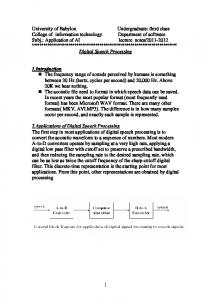


![[PDF] Online Digital Speech Processing Using Matlab ... - Google Sites](https://m.moam.info/img/260x300/pdf-online-digital-speech-processing-using-matlab-_647708e2097c474b228b8484.jpg)