|
Royal Swedish Academy of Sciences
Physica Scripta
Phys. Scr. 90 (2015) 085401 (8pp)
doi:10.1088/0031-8949/90/8/085401
Spherically symmetric states of Hookium in a cavity Vladimir I Pupyshev1 and H E Montgomery2,3 1
Laboratory of Molecular Structure and Quantum Mechanics, Department of Chemistry, Lomonosov Moscow State University Moscow, 119991, Russia 2 Chemistry Program, Centre College Danville, KY 40422, USA E-mail:
[email protected] and
[email protected] Received 12 March 2015, revised 7 May 2015 Accepted for publication 21 May 2015 Published 2 July 2015 Abstract
When a two-electron atom or ion is enclosed in an impenetrable spherical cavity, level crossings and avoided crossings are observed as the cavity radius changes. The locations of those crossings depend on the cavity radius and the nuclear charge of the system. The question arises as to whether this crossing behavior is unique to the one-electron Coulomb potential or whether it can be observed in other confined single-particle electron potentials. In this work we examined some low-lying singlet and triplet states of two-electron systems with isotropic harmonic singleparticle 3D potentials. The spherically symmetric S states are analyzed using variational energies calculated with Hylleraas-type function. The energy dependence of low-lying states is considered as a function of the cavity radius and the harmonic force constant. For positive force constants, there exist cavity radii where the 21S and 13S states are degenerate. Analogous points do not exist for the two-electron quantum dot where the one-electron potential corresponds to an infinite rectangular box. The structure of the energy spectrum for negative force constants is also studied. The similarities and differences of the two-electron S states for the Coulomb and harmonic potentials are considered. Keywords: harmonic oscillator, electronic structure, excited states, variational method, Hookium (Some figures may appear in colour only in the online journal) 1. Introduction
become a very important model in atomic quantum mechanics, see e.g. [4–9] and references therein. These systems are usually called Hookium or Harmonium. Here we prefer to use Hookium, as the alternative term ‘Harmonium’ is often used in the literature for another system, the so called Moshinsky atom (see e.g. [1], ch. V.24 or [10]) where both the electron–nuclear and electron–electron interactions are harmonic. Later, special names were proposed for two-electron systems with a one-particle potential of the form Kr n [11, 12]. For example, the two-electron system in an impenetrable spherical cavity was called ‘Ballium’ [11]. The other name of the system is ‘quantum dot’, but this term is excessively general. The external one-particle harmonic potential was natural in the theory of quantum dots and similar systems [13, 14] but correlation of the force constant with the quantum dot radius is not at all trivial. For the theory of quantum dots see [15–20] and references therein. Nowadays the external harmonic field
Nowadays it is practically impossible to describe all of the applications of harmonic oscillators in theoretical problems, though there have been attempts to realize that goal [1]. The idea to use harmonic oscillators to model electron correlation effects was proposed in [2] where the system of two particles in the field of the isotropic harmonic one-particle potential r2 K 2 with a Coulomb interparticle repulsion was described by a pair of independent one-particle equations. A general solution of the corresponding radial equations for the relative coordinate is only possible numerically. It was later found that for some cases the wave functions can be expressed in analytic form. Much later, it was explained that this is the consequence of a hidden symmetry of the system [3]. The twoelectron system with a harmonic one-particle potential has 3
Author to whom any correspondence should be addressed.
0031-8949/15/085401+08$33.00
1
© 2015 The Royal Swedish Academy of Sciences
Printed in the UK
Phys. Scr. 90 (2015) 085401
V I Pupyshev and H E Montgomery
is frequently used to model confined atoms or molecules [21– 24]. Harmonic confinement is also interesting for systems with a larger number of electrons [25]. We have previously shown [26] that when one considers the states of a He atom in an impenetrable spherical cavity, it is possible to find cavity radii where the singlet and triplet S states, 21S and 13S, are degenerate. Our studies of other atomic states confirm the general character of this situation for 2e systems, though for ballium we cannot find similar degeneracies for the 13S and 21S states [27]. In the present work we sought to determine the extent to which the singlet–triplet degeneracies are the result of the Coulomb nature of the electron–nuclear interaction and if they can be reproduced in other systems. As will be shown below, Hookium in an impenetrable spherical cavity is one of the difficult cases of the problem. Hence, the possibility of using the harmonic model for an external potential in 2equantum dots requires special analysis to distinguish the real physical effects of the cavity size from the influence of the harmonic cavity-potential.
in the literature for enumerating the states (e.g. for vibrational problems the numbers v = 0, 1,… are more traditional while for atomic systems the hydrogen-like tradition requires n > ℓ ). We used the numerical CI algorithm to interpret the results of much more exact Hylleraas basis set calculations. The traditional algorithms were used here for small size CI calculations with 15–20 configuration functions of fixed spin and momentum state (see [26, 27]). The step size ∼10−3a0 is sufficient for stable numerical evaluation of two-electron integrals. In energy accuracy of this crude method is less than the Hylleraas calculations and varies from very small values for small cavities to errors of the order 10–2 Eh for R ∼ 5 a0. Nevertheless the configuration weights are stable enough to illustrate the essential changes in the wave functions. According to angular momentum theory, for S states with zero total electronic angular momentum only two-electron configurations of the form nℓn′ℓ with identical momenta of both electrons shall be considered (see ch. XIV, section 106 in [30]). Due to the symmetry properties of the 3j-symbols, the angular parts of the two-electron S functions do not change under permutation of the electron variables. This is also evident from the explicit form of the angular parts of two-electron configurations for S states (see e.g. equation (32) in [31]). This explains why for S states there exist only singlet states with configurations nℓ 2 while for n ≠ n′ both triplet and singlet configurations may be considered.
2. The methods used For numerical estimates we used the wave functions constructed in the Hylleraas coordinates defined by the distance rj = |rj| from the jth electron to the center of the spherical cavity, where the coordinate system origin is placed and the interparticle distance r12 = |r1–r2|. The wave functions were expansions of the form
3. Qualitative description of the problem In order to consider the state ordering of confined Hookium with respect to confinement radius R we consider two limiting cases: the limit of small cavities R → 0 and the limit of large cavities R → ∞. The discussions of this kind can be realized in a number of independent constructions. One can use transformations of the Hamiltonians of the systems studied, that have the form (here and later only atomic units are used; for example, we use atomic Bohr radius a0 for distances and atomic Hartree units Eh for energy)
⎤ N ⎤⎡ ⎡ 1 1 ψ N = ⎢ R − (s − t ) ⎥ ⎢ R − (s + t ) ⎥ ∑ck s l k t m k un k , (1) ⎦ ⎦⎣ ⎣ 2 2 k=1
where s, t and u are the Hylleraas coordinates defined by s = r1 + r2;
t = −r1 + r2;
u = r12.
(2)
The ck s are variational parameters determined by minimizing the calculated energy. The factors ⎡ R − 1 (s ± t ) ⎤ are cutoff functions that insure that the ⎣ ⎦ 2 wave function goes to zero at R, the radius of the confining cavity. The wave functions included all terms with l k + m k + n k ⩽ 8 subject to the requirement that mk = even for the singlet state and mk = odd for the triplet. The resulting wave functions thus included 95 terms. Convergence studies using a 125-term wave function indicated that our results are stable, in at least the third decimal place. The methods used to evaluate the Hamiltonian’s matrix element are described in [28, 29]. See also [26, 27] for other details of the numerical procedures used here. The qualitative interpretation of the results is given here in terms of a configuration interaction (CI) wave function. The one-electron states corresponding to the one-particle potential are enumerated as nℓ, where n is the ‘main quantum number’ and ℓ defines the angular momentum. Here we use the independent numeration for states with any momentum: n = 1, 2,…, though there exist a number of different traditions
r 2 + r22 1 1 1 H = − Δr1 − Δr2 + K 1 + . 2 2 2 r12
(3)
It is easy to show that after a scale transformation, one can consider the Dirichlet problem in a sphere of radius 1 with 1 a Hamiltonian of the form 2 HR, where R
r 2 + r22 1 1 R HR = − Δr1 − Δr2 + R 4K 1 + . 2 2 2 r12
(4)
Discussion of similar problems is traditional in quantum mechanics (see e.g. [32–34] and applications to simple potentials in [27, 35, 36]). Here it is important that the energy values E(R) for the Dirichlet problem in the sphere of radius R define the energy levels for the Hamiltonian HR (4) as R2E(R). In particular, relation (4) makes clear the use in literature of values ∼K–1/4 (or ∼ω–1/2) as a measure of the cavity radius 2
Phys. Scr. 90 (2015) 085401
V I Pupyshev and H E Montgomery
R for models of the potential of an impenetrable spherical cavity by external isotropic harmonic potential with force constant K (or frequency ω = K1/2). This model is considered as traditional, at least from the time of the papers [13, 14].
Hence, the configurations of the low-lying unperturbed S states are ordered as 1s2 ,
3.1. Small cavities
( ) 1s3s ( 7 S, 3 S) … .
)
1s2 11S , 1p2 21S , 1s2s 31S, 13 S , 1d2 41S , 2
1
1
3
1
3
2
} {1p2p,
1s2s ,
}
2s2 , 1d2 , 1s3s … .
(8)
Due to the high density of the states, it is difficult to estimate the relative positions of the states with different configurations without tedious calculations. This is why we use the modified form of the problem, known for the free Hookium from the first works [2, 4, 5]. It is much simpler to use perturbation theory after unitary transformation of variables from r1,2 to s± = ( r1 ± r2) / 2 (the traditional Jacobi coordinates also may be used here). The problem with the Hamiltonian H is transformed for new variables to a pair of independent problems. The variables s+ describe the motion of the center-of-mass by a 3D isotropic oscillator with force constant K. The solution of this problem is known. The variables s– correspond to the spherically symmetric 3D problem of relative motion of particles in the 1 same harmonic potential perturbed by the operator . The
For cavities of small radius, it is clear from the form of HR that one can ignore the potential energy terms in comparison with the kinetic energy. This is a known feature of small cavities; see e.g. [36] or the detailed discussion in [37]. In the small R limit the problem reduces to a description of the independent motion of two free electrons in a spherical cavity. This is a problem from textbooks; see e.g. problem 62 in [38] or ch. V, section 33 in [30]. As a result, one can find the ordering of the low-lying S states of Hookium for small R as
( ) ( ) ( 2s ( 5 S) , 1p2p ( 6 S, 2 S),
{1p ,
(5)
2 s−
methods for solution for this problem and its analysis can be found in the above mentioned classic works on Hookium and in [41]. When one uses perturbation theory to estimate the energies of the harmonic oscillator perturbed by the field like |s–|–1, it is easy to find that the first-order energy corrections to the radial problems of the states 1s, 2s and 1p are related as 6:5:4. It follows from these relations that
It is natural that the configurations presented give the main contributions to the corresponding wave functions of Hookium states for small R values. In particular, for small R values, one can use Hund’s rule for the states of the same configuration, for example, using Slater’s arguments [39, 40]. One can insist that the state 13S with configuration 1s2s has a lower energy than the 31S singlet state with the same configuration and the state 23S (1p2p) is lower than 61S (1p2p).
1s s_ –1 1s :
3.2. Large cavities
= 6: 5: 4.
For the positive force constant K, increasing the cavity radius gives the energy levels converged to the levels of the free problem (for discussion of the problem and literature see [36]). It should be noted that formal manipulations with the relation of different terms in the potential of the Hamiltonian HR can be dangerous. Nevertheless, for large enough values of the force constant K and a fixed R value, one can consider the interparticle repulsion as a perturbation being relatively small in comparison with the harmonic potential. The unperturbed Hookium problem corresponds to the system of two independent oscillators. Remember that the spectrum of the isotropic harmonic oscillator problem is known (see problems 65, 66 in [38]). For the systems considered here, the state nℓ corresponds to the stationary energy level ⎛ 1⎞ (3DHO) εnℓ = ℏω ⎜ 2 n + ℓ − ⎟ ⎝ 2⎠
(n = 1, 2, …),
2s s_ –1 2s :
1p s_ –1 1p (9)
For the simple relations and tables needed to calculate the mean values for the 3D isotropic harmonic oscillator see, e.g. section 3 of [42] and section 1.2 in [1]. Hence, the four lowest two-electron S states of Hookium (including those degenerate in the unperturbed problem) may be ordered as 1s & 1s, 1p & 1p, 1s & 2s and 2s & 1s, where the first state symbol corresponds to the s+ variable and the second one describes s–. Note that while the rotational symmetry of the two-electron wave-function can be described by the usual theory of angular momentum, the symmetry of the spatial part with respect to permutation of the particles is defined by the parity of its s– part with respect to the inversion s– → −s– (the s+ variables do not change under electron permutation). Hence, the lowest states for free Hookium are ordered as 11S, 13S, 21S, 31S. One may question if perturbation theory can be used for the case of small force constant, K. To answer this question, let us consider the limiting case K → 0 that allows consideration of the lowest degrees of K in all relations. The corresponding calculations and asymptotic representations for all the terms considered below are described in detail in [5, 6], but our problem is much simpler and we only stress the main idea. The radial part of the potential in the relative coordinate
(6)
where ω = K is the classical oscillator frequency. The lowest one-particle states are ordered as 1s, 1p, {2s, 1d}, {2p, 1f}… (here and later the curly brackets denote systems of degenerate or almost degenerate states). For the unperturbed two-electron system, the S states with configurations nℓn′ℓ have the energies (3DHO) E nℓ, n ′ ℓ = εnℓ + εn(3DHO) = ℏω (2(n + n′ + ℓ ) − 1) . (7) ′ℓ
3
Phys. Scr. 90 (2015) 085401
V I Pupyshev and H E Montgomery
s = |s–| has the form V (s) =
g K + s2 s 2
confinement radius R*. In [26, 27] we have demonstrated the similar phenomenon for confined atomic systems with the Coulomb one-particle potential. It is important for us that the 13S/21S degeneracy exists for any positive K value, but its location R* increases monotonically as the force constant decreases. It is worth noting once more, that when one considers the electronic states 13S and 21S, for small spherical cavities for any electron–nuclei interaction, the lowest triplet state may be described by the configuration 1s2s, while the lowest excited singlet S state has the configuration 1p2. For small cavities, the one-electron 1p state always lies much lower in energy than 2s and the states are ordered in energy as 21S, 13S. For the case of large cavities one may use the estimates for the free systems state ordering. For example, for He-like systems with the Coulomb electron–nuclear interaction it was almost evident, that the one-electron states 1p and 2s have identical energies and the 21S state has configuration 1s2s, just as 13S. In accordance with Hund’s rule, the state ordering is modified for the free system to 13S, 21S. This requires the existence of the degeneracy point 13S/21S, as was demonstrated in [26, 27]. The case of the harmonic electron–nuclear interaction is a much more difficult situation, as the free 3D isotropic oscillator one-electron 1p state is much lower than the 2s state and lies exactly at the middle-point between the 1s and 2s states. We have to realize the additional study in the preceeding section of the two-particle state ordering to find that for the free Hookium atom, the state ordering is 13S, 21S both for small and large K limits. This means that the degeneracy point 13S/21S exists for confined Hookium systems, but this situation may be inverted for some higher r n potentials.
(10)
for some constant g. The minimum position corresponds to smin = 3 g /K . The smaller the value of K, the larger is smin. This means that one can ignore the angular momentum dependence of the potential near smin in the first approximation. The second derivative of the potential near the minimum is ∂ 2V 2g ( s min) = 3 + K = 3K . 2 ∂s s min
(11)
Hence one can describe the energy levels of low-lying S states for Hookium with small frequency as (3DHO) E nℓ and Mℓ = εnℓ + ℏω 3 (M + 1/2) + V ( s min)
(
= ℏω 2 n + ℓ +
)
3 M + c′
(12)
with some function of frequency c′ not dependent on the state in the orders lower than ω. The corresponding ordering of the states confirms the perturbation theory estimates. The lowest S states of Hookium are 11S, 13S, 21S, 31S. That is, the structure of the lowest part of the spectrum for Hookium is the same both in the case of large and small force constants. Note that similar, but much more tedious, detailed calculations allow estimation of the energies of many-electron systems in both the small and large K limits for analysis of the energy level structures of more complex systems (see, e.g. [25] and references therein). The similarity in the state ordering for the Hookium lowest states mentioned above for both small and large K values means that one can suppose that there are no degeneracy points for the lowest excited singlet and triplet states 13S and 21S of Hookium in the whole space for any force constants. On the other hand, according to our discussion (see the text below the equation (4)) for the problem in the whole space, the limits of large and small K values can be considered as the limits of small and large R values for the twoelectron system in a spherical box within harmonic approximation of the system. It is important to understand the region of applicability of the harmonic cavity model.
3.4. The case K = 0
One can also consider an interesting situation for ‘Ballium’, the two-electron system in a spherical box (the case K = 0). It was noted above that the R2E(R) values are the eigenvalues of the Hamiltonian HR for the sphere of radius 1. The approximate value of the derivative for R2E(R) with respect to R can be estimated using the Hellmann–Feynman theorem for HR (or within first-order perturbation theory) as the mean value of r12 –1. According to our numerical experiments, the wave functions of the system for small R are almost single-configurational and the nature of the state may be defined in the limit R → 0 described above in detail. As a result, the curves R2E(R) form a set of almost straight lines with respect to R and the slopes of all the curves are positive. In accordance with Hund’s rule one can expect for the triplet states less increase with increasing R than for the singlet states with the same configuration. This note is not too important, but with some exceptions: when one considers the singlet state that is slightly below the singlet–triplet pair, some intersections of potential curves can occur. This is the case for the states with configurations 2s2 1 (5 S) and 1p2p (61S, 23S) for which the values of R2E(R) differ only by ∼0.5Eh in the limit R → 0. As the triplet state growth is small in comparison with that for the singlet state, there exists a degeneracy of the states 51S/23S at R = 1.662 a0
3.3. Some important notes
Now we can compare the state ordering for Hookium in spherical cavities of small and large radii. As was demonstrated, the ordering is transformed from 11S (1s2), 21S (1p2), 13S (1s2s), 31S (1s2s) for small R values to the ordering 11S, 13S, 21S, 31S for large R. Considering energies as functions of R gives the analogs to the potential curves in diatomic molecules. According to the famous ‘non-crossing rule’ [43], the energy curves for the S states of the same multiplicity shall not ‘intersect’ with each other. Nevertheless, for the states of different multiplicity, this is natural in the situation described. There exists an intersection of the energy curves for confined Hookium for 13S and 21S states at some 4
Phys. Scr. 90 (2015) 085401
V I Pupyshev and H E Montgomery
(see [27]). The addition of the one-electron potential of the r2 form K 2 cannot change the picture essentially for small R, but the location of the 51S/23S intersection depends strongly on K as will be demonstrated later. One can consider the degeneracy proved in the previous section for the states 13S and 21S of Hookium for positive K values in a similar way. But such generalizations require care as in the limit R = 0 the corresponding difference of R2E(R) values is large (∼4.0 Eh). More than that, as was noted for the two-electron system in the absence of external fields [27], one can demonstrate the absence of the 13S/21S degeneracy, while this type of degeneracy exists for both Hookium and Coulomb systems with attractive potentials. It must be stressed that the harmonic model of the impenetrable cavity results in the inverted ordering of the 13S and 21S states when R values are estimated by the force constant or frequency for the unbounded problem in the whole space. We have not found other interesting degeneracy points for S states in the low-lying part of the two-electron problem in a spherical cavity for Ballium [27], though for other types of symmetry the degeneracy points exist. See e.g. the numerical estimates in [18]).
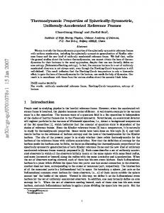
Figure 1. Potential curves for K = 0.005.
uninteresting. For larger K values, the asymptotic behavior of the energy curves can be limited to smaller R values. This is why on the figures presented here, we show R only up to 10 a0 for K = 0.005 and only up to 5 a0 for K = 1. We investigated R values up 20 a0 for K = 0.005 and to R = 8 for K = 1, but the energy changes at these large R values are not visible at the scale of the figures needed to depict the energy changes at smaller R. The nature of the main features of the confined Hookium states for K > 0, like the 13S/21S and 51S/23S degeneracies, were described in detail in previous sections. We describe here mainly the other interesting details. Because the shape of the E versus R curves is relatively insensitive to the value of K and because the separation of states is quite small at any drawing scale that shows the overall curve shape, we only show the curves for K = 0.005, 1 and −1.
3.5. Summary
To summarize the results of this qualitative discussion, we conclude the following: (i) the main configuration of the Hookium state for small R values can be estimated by analysis of the states of two independent particles in the limit R → 0; (ii) at relatively small R, the states 51S/23S can be degenerate; (iii) there exists a degeneracy for the 13S and 21S states, the position of which strongly depends on the positive K values.
4.1. K = 0.005
Figure 1 shows the curves of E versus R for the first six singlet and triplet states over a range of confinement R = 0–10 a0. For small K the system of the states is similar to that for the case K = 0, but the 13S (1s2s) and 21S (1p2) are degenerate at R = 9.38 a0. It is interesting that the weights of the main configurations 1p2 and 1s2s for the states 21S and 31S become close to each other only for R ∼ 18 a0. For the pair of states 41S and 51S, the exchange of the types of leading configurations 1d2 and 2s2 occurs near R ∼ 10 a0. It is difficult here to insist on an avoided crossing, but the picture is quite similar to that. As was previously explained, the states 23S and 51S are degenerate at the relatively small value R = 1.68 a0. For R outside the degeneracy point, the 51S state lies above the 23S state by less than 0.02 Eh and the two curves are indistinguishable in figure 1. For the triplet states 23S (1p2p) and 33S (1s3s), an exchange of the leading configurations occurs at R ∼ 17 а0, which is not clear from the potential curves for the states. For
4. Numerical results For Hookium problems, the potential energy curves E(R) or R2E(R) are shifted up with increasing K. The magnitude of the shift depends on the relation of K and R. In any case, the energy shift is much greater for large R. Note also that for large enough R the energy shift of E(R) with respect to the corresponding energy levels of the free system is defined by the rate of decrease of the wave functions of the free system; see e.g. [36, 44, 45]. Hence for R slightly greater than the boundary of the classically forbidden region, the energy values are practically constant. The energy levels correspond approximately to the system of almost equidistant groups of slightly split or quasi-degenerate levels. The distance between the nearest groups is defined by the frequency of the 3D osci llator and may be estimated as ~2 K . The fast decay of the Gaussian-type functions for the free oscillator means that with increasing R, the state-ordering has only minor variations. This renders the large R values rather 5
Phys. Scr. 90 (2015) 085401
V I Pupyshev and H E Montgomery
configurations 1d2d and 2s3s one can find a similar exchange for 43S and 53S states near R ≈ 11 a0. The configurations mentioned make significant contributions in both of the combined states after the ‘quasi-crossing’ points. It should also be noted that the value of the energy of the 51S state is approximately constant for R > 11 a0, while the decreasing of the 33S state energy is notable in this region. As a result, there is a crossing of the potential curves for 51S and 33S states for R = 13.56 a0. Formally, one can describe for large R the state system in the following way: between the two lowest triplet states are located all the singlet states 21S, 31S and 41S. 4.2. K = 0.01
Increasing K from 0.005 to 0.01 basically shifts the E versus R curves up and compresses them to the left in accordance with results of [27] for homogeneous potentials. The degeneracy of the states 13S (1s2s) and 21S (1p2) occurs at R = 8.05 a0, although the weights of the leading configurations 1p2 and 1s2s for the states 21S and 31S become close to each other only in the region R ∼ 10 a0. In accordance with the Hellmann–Feynman theorem, the energy derivative with respect to K is positive. Together with the tendency toward degeneracy of the states 23S and 51S, this gives potential curves that almost touch each other near the point R = 8.05 a0. There is no reason to analyze this behavior in detail as the results are too sensitive to the level of approximations used. This is the main difference in the structure of the states systems for K = 0.005, 0.01 and larger values. One can find the effect of avoided crossing for the states 41S (1d2) and 51S (2s2). This is connected with the degeneracy of 51S and 33S states for relatively large R. It is interesting that in the same region near 10 a0 the weights of configurations 1d2d and 2s3s become close for both states 43S and 53S where they are simultaneously the leading configurations.
Figure 2. Potential curves for K = 1.
Figure 3. R2E curves for K = –1.
4.5. Negative K
Let us consider the inverted oscillator, that is the system where K < 0. The spectrum of the free system is unbounded and purely continuous. On the contrary, for the confined system there exists only a discrete spectrum. It should be noted that the derivative with respect to R at R = 0 is positive for R2E(R) as it is defined by the 1/r12 mean value only, being independent of K (see equation (4)). This is why the values of R2E(R) increase with R at small R values. The decrease of R2E(R) for large R is evident and can be seen in figure 3 where we have plotted R2E(R) versus R for K = −1 in order to highlight the differences in the behavior of the states for small R. The main features of the inverted oscillator occur at relatively large R. We find that there is no 13S/21S degeneracy, but for K = –1 the states 23S (1p2p) and 51S(2s2) are degenerate at R = 1.24 a0, analogous to the case of the 2e quantum dot (K = 0, Ballium, see [27]). It is more interesting that there exists a second 23S/51S degeneracy at R = 2.88 a0. Approximately the same confinement radius, R ≈ 2.9 a0, corresponds to the avoided crossing of the states 31S (1s2s)
4.3. K = 0.25
As a whole, the picture of the states is similar to that for smaller K values. Degeneracy of the states 13S (1s2s) and 21S (1p2) occurs at R = 3.96 a0. For the states 23S(1s3s) and 51S (2s2) degeneracy occurs at R = 4.40 a0. Near this point at R = 5.34 a0 is the degeneracy point for 33S and 51S states. 4.4. K = 1.0
With increased K the grouping of the states into almost equidistant values at large R is much more obvious as shown in figure 2. The system of states is organized like the case of smaller K, but degeneracy of the states 13S (1s2s) and 21S (1p2) occurs at R = 2.91 a0. Energy differences for the states (2,3)3S and 51S are relatively small for small R and after the 23S/51S degeneracy point at 3.26 a0. At the next crossing point (R = 3.86 a0 ) the 51S state is degenerate with 33S. 6
Phys. Scr. 90 (2015) 085401
V I Pupyshev and H E Montgomery
and 41S (1d2). After this avoided crossing, the state 31S (1d2) decreases at a relatively high rate. For R > 3.0 a0 it lies below the first triplet S state, 13S. Note also, that in the region R ∼ 3.5 there exists for K = –1 an avoided crossing of the states 41S (1s2s) and 51S (at this point the leading configuration of the state is 1f2) resulting in near degeneracy of the states 51S and 13S with the same configuration 1s2s, while the singlet states from 11S to 41S are below all of the triplet states. The corresponding leading configurations of the lowest singlet states mentioned are 1s2, 1p2, 1d2, 1f2. Formally this picture may be described as systematically pushing up of all the triplet levels by the singlets with configurations 1ℓ 2. One can understand this as a general tendency. When the repulsive potential is strong enough for large R values, the lowest state one-electron wave functions are localized near the walls of the cavity. For large cavity radius, R, this means that the angular dependence of the energy levels is of the order ℓ (ℓ + 1) /R 2 . Hence, we find that the lowest one-particle states are 1s, 1p, 1d…. The corresponding two-electron configurations of S type are 1s2, 1p2, 1d2,… that correspond to the singlet states only, as was explained above. Note also that the singlet and triplet states with the same configuration, for example, 1s2s, differ in energy, in Slater’s description, by the exchange integral, that will be small for large R, as the one-electron functions are spread out near the surface of a sphere of large radius. That is, when K < 0 and R is large, the triplet states are almost degenerate with some of the singlet states, while the lowest S states correspond to singlet states of nℓ 2 type. This qualitative description is natural if one notes that for spherium, the 2e-system on the surface of a sphere, only singlet S states are realized due to the Pauli principle (see e.g. [31, 46]). A similar, though more smooth picture was noted for the Coulomb atomic systems with negative nuclear charges [27]; for the Hook’s potential the picture is more clear.
R* = 9.38, 8.05, 3.958, 2.907 a0 for K = 0.005, 0.01, 0.25 and 1.0. Correspondingly, that may be described as R* = 2.913/ K0.221 with the correlation factor R2 = 0.999. One should remember that for a particle in an isotropic harmonic potential, one can estimate the mean value of the distance from the center as ∼K–1/4. When K < 0, there are no degeneracy points of the type 13S/21S. The case K = 0 corresponds formally to the boundary case when R* is infinite. One must stress that the degeneracy points for simple systems are interesting from several points of view. Such points are important to analyze the intra-system energy evolution with changing confinement. But it is also important that the degeneracy points form a system of reference points to give a qualitative picture of the states when one considers variation of the external parameters. And last, these characteristic points of the system give a natural basis for comparison of the accuracy of approximate models and numerical methods used for confined system analysis. For example, our study shows clearly that when one uses the harmonic model of the spherical confinement, some essential effects like changes in 13S/21S state ordering may appear in comparison with ‘the infinite rectangular box’. Of course, the importance of similar effects and possibility of the use the corresponding models in real physical studies depends on the physical problem under consideration.
Acknowledgments HEM thanks the Centre College Faculty Development Fund for financial support. VIP thanks the Russian Foundation for Basic Research (Project No. 13-03-00640a) for support.
References 5. Discussion
[1] Moshinsky M 1969 The Harmonic Oscillator in Modern Physics: from Atom to Quarks (London: Gordon and Breach) [2] Kestner N R and Sinanoglu O 1962 Study of electron correlation in helium-like systems using an exactly soluble model Phys. Rev. 128 2687–92 [3] Turbiner A 1994 Two electrons in an external oscillator potential: the hidden algebraic structure Phys. Rev. A 50 5335–7 [4] Kais S, Herschbach D R and Levine R D 1989 Dimensional scaling as a symmetry operation J. Chem. Phys. 91 7791–6 [5] Taut M 1993 Two electrons in an external oscillator potential: particular analytic solutions of a Coulomb correlation problem Phys. Rev. A 48 3561–6 [6] Taut M 1994 Two electrons in a homogeneous magnetic field: particular analytical solutions J. Phys. A: Math. Gen. 27 1045–55 Taut M 1994 J. Phys. A: Math. Gen. 27 4723–4 (erratum) [7] Cioslowski J and Pernal K 2000 The ground state of Harmonium J. Chem. Phys. 113 8434–43 [8] Varga K, Navratil P, Usukura J and Suzuki Y 2001 Stochastic variational approach to few-electron artificial atoms Phys. Rev. B 63 205308
As a whole, the system of spherically symmetric S states for confined Hookium is much simpler than that for confined atomic systems [26, 27]. The main features of the low lying states are defined by the behavior of two almost free electrons in small cavities and the state grouping in the limit of large R. There are important points of degeneracy in the 23S and 1 5 S states that are usually realized for small cavities, but sometimes the energy curves are too close to be stable to small external perturbations or numerical errors. The degeneracy points of the states 13S (1s2s) and 21S (1p2) have a more general character for the case K > 0 (the similar intersection of potential curves for the case of K ⩽ 0 does not exist). As follows from the scaling properties of the potentials, the growth of the positive K values corresponds to the formal compression of the potential curves picture (see details in [27]). One can see this formally by analyzing the 13S/21S degeneracy point R* as a function of R. Really, we have 7
Phys. Scr. 90 (2015) 085401
V I Pupyshev and H E Montgomery
[27] Montgomery H E and Pupyshev V I 2015 Confined twoelectron systems: excited singlet and triplet S states Theor. Chem. Acc. 134 1598 [28] ten Seldam C A and de Groot S R 1946 On the energy levels of a model of the compressed hydrogen atom Physica 12 669–82 [29] Pan X-Y, Sahni V, Massa L and Sen K D 2001 New expression for the expectation value integral for a confined helium atom Theor. Comput. Chem. 965 202–5 [30] Landau L D and Lifshitz E M 1977 Quantum Mechanics: NonRelativistic Theory vol 3 (New York: Pergamon) [31] Loos P-F and Gill P M W 2009 Ground state of two electrons on a sphere Phys. Rev. A 79 062517 [32] Fock V 1930 Bemerkung zum virialsatz Z. Phys. 63 855–8 [33] Kais S and Serra P 2003 Finite-size scaling for atomic and molecular systems Advances in Chemical Physics vol 125 ed I Prigogine and S A Rice (Hoboken, NJ: Wiley) pp 1–99 [34] Patil S H and Varshni Y P 2006 Two electrons in a simple harmonic potential Can. J. Phys. 84 181–92 [35] Pupyshev V I and Stepanov N F 2014 Spectroscopic characteristics of simple systems in a spherical cavity Russ. J. Phys. Chem. 88 1882–8 (Engl. transl.) [36] Sen K D, Pupyshev V I and Montgomery H E 2009 Exact relations for confined one-electron systems The Theory of Confined Quantum Systems, Part I Advances in Quantum Chemistry vol 57 ed J R Sabin, E Brändas and S A Cruz (Amsterdam: Academic) pp 25–77 [37] Fernandez F M 2014 Perturbation theory for confined systems J. Math. Chem. 52 174–7 [38] Flügge S 1971 Practical Quantum Mechanics I (Berlin: Springer) [39] Slater J C 1929 The theory of complex spectra Phys. Rev. 34 1293–322 [40] Kutzelnigg W and Morgan J D 1996 Hund’s rules Z. Phys. D 36 197–214 [41] Hall R L, Saad N and Sen K D 2011 Spectral characteristics for a spherically confined −a/r + br2 potential J. Phys. A: Math. Theor. 44 185307 [42] Brody T A, Jacob G and Moshinsky M 1960 Matrix elements in nuclear shell theory Nucl. Phys. 17 16–29 [43] von Neumann J and Wigner E 1929 Über das verhalten von eigenwerten bei adiabatischen prozessen Physikalische Zeitschrift (Leipzig) 30 467–70 [44] Hull T E and Julius R S 1956 Enclosed quantum mechanical systems Can. J. Phys. 34 914–9 [45] Wilcox W 2000 Finite volume effects in self-coupled geometries Ann. Phys. 279 65–80 [46] Loos P-F and Gill P M W 2010 Excited states of spherium Mol. Phys. 108 2527–32
[9] Gill P M W and O’Neill D P 2005 Electron correlation in Hooke’s law atom in the high-density limit J. Chem. Phys. 122 094110 [10] Santos E 1968 Calculo aproximado de la energia de correlation entre dos electrons An. Fis. 64 177–93 [11] Loos P-F and Gill P M W 2009 Correlation energy of two electrons in the high-density limit J. Chem. Phys. 131 241101 [12] Loos P-F and Gill P M W 2010 A tale of two electrons: correlation at high density Chem. Phys. Lett. 500 1–8 [13] Maksym P A and Chakraborty T 1990 Quantum dots in a magnetic field: role of electron–electron interactions Phys. Rev. Lett. 65 108–11 [14] Merkt U, Huser J and Wagner M 1991 Energy spectra of two electrons in a harmonic quantum dot Phys. Rev. B 43 7320–3 [15] Bednarek S, Szafran B and Adamowski J 1999 Many-electron artificial atoms Phys. Rev. B 59 13036–42 [16] Johnson N F 1995 Quantum dots: few-body, low-dimensional systems J. Phys.: Condens. Matter 7 965–89 [17] Thompson D C and Alavi A 2002 Two interacting electrons in a spherical box: an exact diagonalization study Phys. Rev. B 66 235118 [18] Jung J and Alvarellos J E 2003 Two interacting electrons confined within a sphere: an accurate solution J. Chem. Phys. 118 10825–34 [19] Prudente F V, Costa L S and Vianna D M 2005 A study of two-electron quantum dot spectrum using discrete variable representation method J. Chem. Phys. 123 224701 [20] Ciftja O O 2013 Understanding electronic systems in semiconductor quantum dots Phys. Scr. 88 058302 [21] Sabin J R, Brändas E and Cruz S A (ed) 2009 The Theory of Confined Quantum Systems, Parts I and II Advances in Quantum Chemistry vol 57, 58 (Amsterdam: Academic) [22] Sen K D (ed) 2014 Electronic Structure of Quantum Confined Atoms and Molecules (Heidelberg: Springer) [23] Sako T and Diercksen G H F 2008 Understanding the spectra of a few electrons confined in a quasi-one-dimensional nanostructure J. Phys.: Condens. Matter. 20 155202 [24] Sako T, Paldus J and Diercksen G H F 2014 Angular correlation in He and He-like atomic ions: a manifestation of the genuine and conjugate fermi holes Phys. Rev. A 89 062501 [25] Cioslowski J, Strasburger K and Matito E 2014 Benchmark calculations on the lowest-energy singlet, triplet, and quintet states of the four-electron Harmonium atom J. Chem. Phys. 141 044128 [26] Montgomery H E and Pupyshev V I 2013 Confined helium: excited singlet and triplet states Phys. Lett. A 337 2880–3
8