αSPIN: A tool for abstract model checking - CiteSeerX

Int J Softw Tools Technol Transfer (2004) 5: 165–184 / Digital Object Identifier (DOI) 10.1007/s10009-003-0122-9

αSPIN: A tool for abstract model checking Mar´ıa del Mar Gallardo, Jes´ us Mart´ınez, Pedro Merino, Ernesto Pimentel∗ Dpto. de Lenguajes y Ciencias de la Computaci´ on, University of Malaga 29071 M´ alaga, Spain e-mail: {gallardo,jmcruz,pedro,ernesto}@lcc.uma.es Published online: 9 December 2003 –  Springer-Verlag 2003

Abstract. Abstraction methods have become one of the most interesting topics in the automatic verification of software systems because they can reduce the state space to be explored and allow model checking of more complex systems. Nevertheless, there is a lack of tools actually supporting this technique. One direction for abstracting a system is to transform its formal description (its model) into a simpler version specified in the same language, thus skipping the construction of a specific (model checking) tool for the abstract model. The abstraction of the model should be followed by the abstraction of the temporal formulas to be checked. This paper presents αspin, a tool for the integration of abstraction (for models and formulas) into the well-known model checker spin. We present the theoretical results supporting the implementation together with a case study. Keywords: Verification – Model checking – Abstraction – spin – Temporal logic

1 Introduction Automatic verification methods such as model checking [4] have become realistic techniques to be used in the development of critical systems. However, model checking is only effective when a useful model of a system is available. By useful we mean an abstract representation of the system, containing only the details that ensure that satisfaction (nonsatisfaction) of certain properties provides us with information about the actual behavior of the system. Models describing an excess of details may produce the state explosion problem, which could prevent the use of ∗ Work supported by projects TIC2002-04309-C02-02 and TIC20012705-C03-02

current tools to fully analyze them. This problem affects both the symbolic method and explicit model checking. In [32] it was recently acknowledged that model checking may profit from its combination with abstract interpretation [9] to reduce the size of models. However, this technique is not new; the first papers formalizing and studying the main problems of abstract model checking were presented by Clarke et al. [5], Loiseaux et al. [41], Graf et al. [28], and Cleaveland et al. [8], to mention a few. Applying abstract model checking involves different steps, as enumerated in [5]. First, the original model, also called the concrete model, must be reduced. To achieve this, we abstract the meaning of some “selected” data types in the concrete model. This abstraction may be done using “abstraction functions” [5, 10, 16], as in the typical applications of abstract interpretation, and also by means of so-called “predicate abstractions” [1, 28, 43]. Second, once the abstract model has been constructed, it is necessary to redefine the properties in order to adapt them to the new model representation. The abstract model constructed is, in general, an overapproximation of the concrete one; that is, the new model represents more behaviors due to the loss of information inherent in the abstraction. Therefore, an important point to be studied in abstract model checking is the preservation of the temporal properties from the abstract to the concrete model. Clearly, there exists a tradeoff between obtaining the least abstract model, producing the smallest set of states, and preserving as many of the most important temporal properties as possible. The effective application of the abstract model checking technique involves the construction of tools supporting the automatic abstraction of models and properties. This paper presents αspin [22], a tool integrating abstract model checking into the well-known model checker

166

M. del Mar Gallardo et al.: αspin: A tool for abstract model checking

spin [33, 34]. The main characteristics of the tool are summarized below. αspin realizes a source-to-source transformation of both the original model and the temporal properties. This allows us to reuse the same tool (spin) to verify the abstract model. To construct the abstract model, αspin follows the “abstraction function” method, substituting the type of certain model variables with a simpler abstraction. Users may select the abstraction function to be applied from an abstraction library, as also occurs in [14] or [28]. Correctness conditions, studied in [16], assure that the abstract model generated in this way correctly simulates (overapproximates) the original one. Syntactic transformation makes use of xml [45] as intermediate language [19]. xml-associated tools allow us to easily manipulate the xml descriptions. For instance, we may prove that the new abstract model constructed correctly follows the promela syntaxis using the dtd (document types definition) file. Regarding the abstraction of properties, the classic method [5, 10] underapproximates the formulas in the sense that their meaning is more restrictive. In other words, it is more difficult for an abstract trace to satisfy an underapproximated formula. Informally, we may say that the overapproximation of the model is compensated by the underapproximation of the formulas. Consequently, this method preserves properties from the abstract to the concrete model, that is, it is suitable for checking whether a temporal formula is true for all execution paths in the original model. However, users may also prefer to specify “bad” nondesirable properties by means of temporal formulas that no model trace is expected to verify. In fact, spin itself provides these two functionalities: the verification of desirable (universal) properties and the refutation of nondesirable (existential) properties. It is worth noting that spin implements on-the-fly automaton-based model checking following [24], which means that nondesirable properties are directly translated into the automaton, but universal properties have to be negated (transformed into nondesirable ones) before being translated. While in the concrete world the negation of a desirable property gives us the corresponding bad property to be refuted, and vice versa, this transformation is not so direct for abstract properties. The reason for this is that the abstraction process affects the evaluation of negated atoms. Therefore, we may say that, in general, the underapproximation of a (negated) formula cannot be used directly to refute a property. One clear possibility for dealing with the refutation of abstract properties is trying to prove the (universal) satisfiability of the negation of the formula to be refuted using the underapproximated approach. This method involves the negation of the existential formula and its transformation into the normal negation form to obtain the input for spin. Note that spin would translate once again the new constructed formula into its negation.

A different alternative that avoids the first transformation (not implemented in spin) consists in defining a new satisfaction relation specifically oriented to refuting abstract properties. In [18, 21], we proved that the dual approach to abstracting properties based on overapproximation, reusing the same technique followed for abstracting the model, can also be employed effectively in abstract model checking. This approach naturally preserves the refutation of existential temporal formulas from the abstract to the concrete model. Similar operators for dealing with negation in the abstract world have also been introduced in [38–40]. In addition, in [23] we proved that these methods are effectively dual in the sense that the above-mentioned equivalence between verification and refutation is achieved by using the under and over interpretations, respectively. Actually, these two approaches can be considered as the two sides of the same coin, but special care is necessary to “turn the coin over”. Apart from saving on development efforts, users may benefit from having two ways of interpreting abstract formulas. They can directly write the properties with the (abstract) interpretation best suited for the goal. Furthermore, these two points of view have also allowed us to obtain more benefits for refining the abstract model, as studied in [23]. The elimination of “spurious traces” (no realistic traces) from the abstract model is one of the major challenges in abstract model checking. These false traces may lead to obtaining false negatives, making the abstract analysis useless. Solutions of this problem are based on the analysis of counterexamples to find out whether they are real or fictitious [6, 42, 43]; on model refinement as in [10]; or on the application of general results about the incompleteness problem in abstract interpretation [25] to the case of abstract model checking [26]. Our proposal, however, uses the combination of the two methods to construct formulas that simultaneously represent the property to be checked (or refuted) and the part of the model that has to be analyzed to safely prove it. In other words, we make use of the model checking power to automatically refine the model. As a consequence, this method is particularly appropriate for on-the-fly model checking [7] as implemented in spin. Abstract model checking is also supported by other tools that are mainly oriented to programming languages and not to formal description techniques. The closest tool to αspin is Bandera [14, 30] which takes a Java program and produces a verification-oriented model written in the input language of tools like spin or JPF [44]. Bandera employs dependency analysis to find further variables to be abstracted and integrates powerful features like slicing or automatic support to construct sound abstraction functions (with the assistance of the theorem prover PVS). Bandera finds spurious counterexamples, making sure that the counterexample contains no nondeterministic assignments [42]. αspin shares with Bandera the data abstraction method based on the use of the abstraction library to produce an overapproximated

M. del Mar Gallardo et al.: αspin: A tool for abstract model checking

model. αspin offers some features that differ from Bandera’s, like several choices for constructing the abstract model for a given abstract function, the use of under- or overapproximation of formulas at the user level, or dealing with the problem of spurious counterexamples by refining the properties [23]. Other closely related projects where data abstraction is considered are FeaVer [37] and abC [12]. FeaVer produces a promela model from annotated ANSI C code. It employs a lookup table to map C instructions into promela. This mapping, for example, permits removing or reducing the range of selected variables, producing an effect similar to data abstraction. abC extends the compiler gcc with the ability to hide variables in such a way that the new C code must include nondeterministic expressions to overapproximate the initial program. A different approach to abstract model checking tools is to construct specific model checkers that support abstraction rather than reusing existing model checkers. This is the idea of Java Path Finder (JPF) [3, 44] and SLAM [2], which are based on the predicate abstraction technique introduced in [29]. This technique consists in replacing some user-selected predicates with Boolean variables in such a way that the abstract model is a safe overapproximation of the concrete one. JPF is an evolution of JPF1 [31]. JPF1 used a translation from Java to promela, including the abstraction in the translation phase. JPF is a model checker that works at the Java bytecode level. It supports predicate abstraction by automatically translating an annotated Java program to another Java program. The goal of SLAM is to check temporal safety properties of sequential C programs, transforming the C program into a Boolean program that preserves all controlflow constructs, but only Boolean variables. See [11] for a more extended survey of abstraction techniques and associated tools. The paper is organized as follows. Section 2 contains some preliminary background on spin and its input languages. Sections 3 and 4 present the theoretical basis for supporting correct abstraction by transformation of promela and temporal logic, respectively. In Sect. 5, we explain how to use αspin with a previously published lift controller system as the case study [13]. Section 6 is devoted to some implementation details of αspin. In the last section, we provide conclusions and outline some future work.

2

temporal logic (ltl). It is also used as the platform for trying new powerful algorithms to attack the state explosion problem. 2.1 Modelling with promela promela is a language designed for describing systems composed of concurrent asynchronous communicating processes. A promela model P = P roc1 || . . . ||P rocn consists of a finite set of processes, global and local channels, and global and local variables. Processes communicate via message passing through channels. Communication may be asynchronous using channels as bounded buffers and synchronous using channels with size zero. Global channels and variables determine the environment in which processes run, while local channels and variables establish the internal local state of processes. promela is a nondeterministic language that borrows some concepts and syntax elements from Dijkstra’s guarded command language, Hoare’s CSP language, and C programming language (Fig. 1). A promela process is defined as a sequence of possibly labelled sentences preceded by the declarative part (see example in Fig. 3). Basic sentences in promela are those that produce a definite effect over the model state, in other words, the assignments, the instructions for sending (receiving) messages to (from) channels, and the Boolean expressions, BExp, that include tests over variables and contents of channels. In addition, promela has other nonbasic sentences like the nondeterministic If and Do sentences. 2.2 Temporal logic spin verifies ltl formulas against promela models. Well-formed formulas of linear temporal logic (ltl) are inductively constructed from a set of atomic propositions (in promela, propositions are tests over data, channels, or labels), the standard Boolean operators, and the temporal operators: always “
”, eventually “”, next “O”,

PROMELA, LTL, and SPIN

In the last few years, spin has become one of the most employed model checkers in both academic and industrial areas [33, 34, 36]. It supports the verification of usual safety properties (like deadlock absence) in systems written in the modelling language promela as well as the analysis of complex requirements expressed with linear

167

Fig. 1. Part of promela syntax

168

M. del Mar Gallardo et al.: αspin: A tool for abstract model checking

2.3 spin

Fig. 2. LTL semantics

and until “U”. Formulas are interpreted with respect to model state sequences ti = si
si+1
. . . . Each sequence expresses a possible model execution from state si . The use of temporal operators permits construction of formulas that depend on the current and future states of a configuration sequence. The semantics of ltl is shown in Fig. 2, where p is a proposition and f and g are temporal formulas. For the sake of convenience, we assume that all formulas are in negation normal form, that is, negations only appear in propositions. Note that we have not included a rule defining the satisfaction of a negated formula. Instead, we treat the evaluation of negated propositions independently of their corresponding nonnegated ones. The reason for this will be explained in Sect. 4. The last two rules in Fig. 2 define the semantics of the universal and existential temporal formulas. Note that symbols ∀ and ∃ are not ltl connectives. We use them to simplify the notation. There, M represents the set of execution traces produced by the model.

By default, given an ltl formula, spin translates it into an automaton that represents an undesirable behavior (which is claimed to be impossible). Then, verification consists of an exhaustive exploration of the state space searching for executions that satisfy the acceptance conditions of the automaton. If such an execution exists, then the tool reports it as a counterexample for the property. If the model is explored and a counterexample is not found, then the model satisfies the ltl property as a universal property. The same verification scheme can be employed to check whether a formula can be satisfied by any path (refutation of existential properties). These two ways of using ltl are presented in a user-friendly interface called xspin, as shown in Fig. 3. The first case corresponds to marking “All Executions” and the second one to “No Executions”. Although there are many real examples where verification can be done with standard exhaustive verification, spin also implements optimization techniques to deal with complex systems. Partial order reduction replaces several interleaved sequences of events (sentences) with only one that represents the whole set. State compression reduces the use of memory by compressing the representation of the states without losing information. Bit-state hashing represents states as bits in a hash table, so in many cases the analysis is only partial. Our new tool preserves these optimization techniques. In the rest of the paper, when we use spin we refer to both the command-line-oriented tool and to xspin.

Fig. 3. Lift system model and ltl formula in xspin

M. del Mar Gallardo et al.: αspin: A tool for abstract model checking

3 Abstracting PROMELA The first step for realizing abstract model checking is to reduce the model to be analyzed. In [16], we described a method based on the source-to-source transformation to abstract promela models. The main idea in this work is that for abstracting models, it suffices to replace the original access definitions of some selected data object so that the range of its possible values is shrunk in such a way that the control part of the program (high-level operations like nondeterminism selection and loops, coroutines, and so on) remain unchanged. From a practical point of view, this observation is very important because it allows us to isolate the program points that must be changed when abstracting a model independently of the complexity of the language constructions. In addition, this modular vision facilitates the definition of abstractions, the analysis of the correctness of the abstraction, and even the implementation. In the rest of this section we summarize the theoretical background supporting the source-to-source transformation method. In the presentation, we use the following notation. Given a set S, S ω denotes the set of all infinite sequences that may be built with the elements of S, and ℘(S) is the powerset of S, that is, the set of all its subsets. Let prom denote the set of all promela systems built following the syntax given by Fig. 1. Assuming that State represents the set of all possible system states, we define functions effect : Basic × State → State test : BExp × State → {f alse, true},

(1)

which describe the effect of executing a basic sentence and a test in a given state, respectively. The semantic function G(·, effect , test) : prom → ℘(Stateω )

(2)

associates each promela model M with the subset of state sequences G(M, effect , test) ∈ ℘(Stateω ) representing all possible execution traces generated by M , in which functions effect and test are used when executing a basic sentence or a Boolean expression. Note that functions effect and test represent the standard implementation of the model data types. To simplify the analysis of properties over G(M, effect , test), we must choose an adequate set of reduced states (Stateα , ≤α ) and a state-to-state abstraction function

Structure ((℘(State), ⊆), (Stateα , ≤α ), α, γ) gives us the Galois connection defining the abstract interpretation of the model, where α : ℘(State) → Stateα and γ : Stateα → ℘(State) are defined as α(c) = ∨{s∈c} β(s) and γ(sα ) = {s ∈ State|β(s) ≤α sα }, respectively. Finally, to obtain the abstract behavior of the model we must also define abstract versions of effect and test, that is, functions1 α α effect α o : Basic × State → State α test α o : BExp × State → {f alse, true}

(3)

giving the proper meaning to the basic promela sentences when executed over abstract states. Given the previous discussion, α ω α G(M, effect α o , test o ) ∈ ℘((State ) )

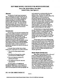
defines an abstract behavior, more easily analyzed, for the same model M . For instance, Fig. 3 shows an excerpt of a promela model that represents the behavior of a lift (extracted from [13]). To simplify the exposition, we assume that system states are given by the value of the variable Position[pid], an integer between the values 0..(nb_floor − 1). That is, in the example State = [0..(nb_ floor − 1)]. Variable Position[pid] always stores the current floor for the lift identified by pid. To reduce the model size, consider the lattice (FLOORS, ≤α ) illustrated in Fig. 4 and the abstraction function β : [0..(nb_floor − 1)] → FLOORS defined as β(0) = Lower β(nb_floor − 1) = Upper β(j) = Middle, ∀0 < j < nb_floor − 1. Note that FLOORS is the set of abstract states (Stateα ) due to the simplification of the model. The use of the partial order ≤α allows us to include the notion of approximation in the abstract domain FLOORS: the abstract value noUpper approximates any floor different from the Upper one; thus noUpper is an abstract value less precise than both Lower and Middle. Value Unknown is the 1 Subindex o denotes that abstract functions overapproximate the original ones. In the following sections, we will also use index u to denote underapproximation.

β : State → Stateα that transforms sets of concrete states into their abstractions. Each abstract datum is intended to represent a set of concrete states sharing some characteristic that is abstracted. (Stateα , ≤α ) is usually a complete lattice, and the partial order ≤α represents the degree of precision of each abstract state.

169

Fig. 4. Lattice FLOORS

170

M. del Mar Gallardo et al.: αspin: A tool for abstract model checking

The way of defining effect α o strongly influences the abstract model constructed, as discussed in the following section. 3.2 Correctness Fig. 5. Part of the abstract effect for FLOORS

least precise abstract datum since it represents any floor. Finally, value ⊥ is used to represent illegal values. The redefinition of states involves the redefinition of the effect of basic sentences. The table in Fig. 5 shows a definition of effect α o : Basic × FLOORS → FLOORS

(4)

for the instructions “increment by one” and “decrement by one”, denoted by inc1 and dec1, respectively.

α β(effect (p, s)) ≤α effect α o (p, s ), α test(b, s) ⇒ test α o (b, s ).

3.1 Power sets as abstract domains The loss of information that occurs when constructing the abstract model may be alternatively represented with sets of abstract values. In this case, the imprecision produced when executing function effect α o is solved by generating the set of the abstract data that can be the result of the function. For example, consider the set AFLOORS = {Lower , Middle, Upper } and let PFLOORS = ℘(AFLOORS). Function effect α o given in Fig. 5 may be redefined as in Fig. 6. Note that the new function effect α o

: Basic × AFLOORS → PFLOORS

(6) (7)

When using Power Sets, the condition set by (6) is replaced by the following one: α β(effect (p, s)) ∈ effect α o (p, s ).

(8)

Correctness conditions guarantee that the abstract model simulates the original one in the sense that for each nondeadlocked trace t = s0
s1
· · · ∈ G(M, effect , test) there exists a nondeadlocked abstract trace α α α tα = sα 0
s1
· · · ∈ G(M, effect o , test o )

(5)

is slightly different from the one given in (4). The difference lies in the way each effect α o function solves the imprecision problem. To explain this, we should note that ideally function effect α o should always return one of the elements of α(State) = {β(s) : s ∈ State}, since this set contains the most precise abstract states (the loss of information in these states is only due to the application of function β.) However, when the result of effect α o cannot be exactly represented with one of these precise abstract data, we may use a domain with imprecise abstract data, as FLOORS in Fig. 5 or, alternatively, construct the set of all possible precise abstract data that can be the result of the function, as in Fig. 6.

Fig. 6. Abstract effect for the lattice PFLOORS

Given an abstraction function β, it is clear that functions α effect α o and test o may be arbitrarily defined. However, the interest of the approach is in preserving some correction properties between the sets of execution traces α G(M, effect , test) and G(M, effect α o , test o ). In [16, 18], there is an exhaustive study of the corα rectness conditions that test α o and effect o must verify for α G(M, effect o , test α o ) to be a correct overapproximation of G(M, effect , test). In summary, these conditions may be written as follows. Given p ∈ Basic and b ∈ BExp and two states s ∈ State, sα ∈ Stateα such that β(s) ≤α sα , then

that overapproximates it. We denote this relation by β(t) ≤α tα , where β(t) = β(s0 )
β(s1 )
. . . , and define it as β(t) ≤α tα ⇔ ∀i ≥ 0 . β(si ) ≤α sα i . For instance, the concrete trace inc1

inc1

dec1

dec1

skip

t= 0
1
2
1
0
... could be approximated by the abstract trace inc1

inc1

tα =Lower
Middle
noLower dec1

dec1

skip


noUpper
noUpper
. . . .

(9)

We have labelled each transition with the basic instruction executed, and we have used the table in Fig. 5 to realize each abstract transition. Note that we explicitly exclude deadlocked traces because the abstraction process may modify this safety property of the system.

M. del Mar Gallardo et al.: αspin: A tool for abstract model checking

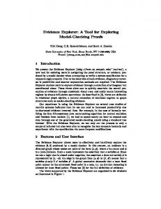
In the previous example (9), we implemented the loss of information when executing abstract operations using specific abstract constants. However, as discussed in Sect. 3.1, we could have used sets of abstract data instead. For example, when the value M iddle is incremented, we could use the set {Lower, M iddle} instead of noUpper . From the implementation point of view, the use of sets implies utilizing nondeterministic assignments when updating abstracted variables, which provokes the direct creation of several branches. Following the example, this means that the abstraction of t produces more than one abstract trace. In Fig. 7, we show the abstract traces in α G(M, effect α o , test o ) overapproximating t, assuming that we have used the definition of effect α o given by the expression (5) and Fig. 6. In contrast, the use of abstract domains defined ad hoc, like (9), eliminates the use of nondeterministic assignments and allows us to delay the creation of branches until a test of the updated variable is found. This means that, in many cases, this method produces smaller abstract models, i.e., it realizes a more effective reduction of the original model. For example, regarding Fig. 7, the abstract model with the specific abstract constants of (9) is smaller than with nondeterministic assignments. In contrast, since the abstract traces are more imprecise, possibly some information relevant for proving certain temporal properties may have been lost. However, in other cases, the use of more values in the abstract domain (seven for FLOORS) than in the power-set-based method (three for PFLOORS or four if the Illegal value is also considered) produces worse results for the first method. In general, the size of the state space for each method depends on how the model produces the values, and we cannot say that one is always better than the other. As both implementation approaches produce correct overapproximations of the model, we have included the two methods as options in αspin, allowing the user to experiment for both a given model and different optimization options. It is worth noting that preventing new nondeterministic sentences in the abstract model permits using the “statement merging” optimization described in [35]. This may be a very interesting point in favor of using the abstract constants method for some systems. When applied to function test, the notion of overapproximation, given by (7), means that function test α o always produces a safe result, that is, it must return true iff in some concrete execution the value true may be re-

171

turned. Thus, given p ∈ BExp, and sα ∈ Stateα , function test α o is defined as
α test α test(p, s)(Over). o (p, s ) = {s∈State.β(s)≤α sα }

In addition, in the following section, we will also make use of this test α o function to implement the overapproximation method for evaluating temporal formulas. 3.3 Syntactic transformation of promela The syntactic transformation of a promela model M to obtain a new model M α is based on replacing each basic instruction in M by a standard promela code that α implements test α o and effect o . Then the verification is carried out by only executing standard promela instructions. This approach corresponds to implementing a verifier for G(M α , effect , test). For instance, the next code shows FLR_INC, a possible implementation of abstract increment inc1 defined in Fig. 5. #define FLR_INCR(x) if :: :: :: :: :: :: fi

x==Lower -> x = Middle \ x==Middle ->x = noLower \ x==noUpper ->x = noLower \ x==noLower ->x = noLower \ x==Unknown ->x = noLower \ else -> x = ILLEGAL \

Following the ideas discussed in the previous sections, it is also possible to implement a different effect α o function, using the table in Fig. 6 as follows. #define FLR_INCR(x) if :: :: :: :: fi

x==Lower -> x = Middle \ x==Middle ->x = Middle \ x==Middle ->x = Upper \ else -> x = ILLEGAL \

In these two codes, the constant ILLEGAL is employed to represent ⊥. The code in Fig. 3 is now replaced by the next one, which illustrates the use of the abstract instruction (effect α o ) to increase the variable Position[]. proctype Lift(int pid){ int Order=null; do ... :: SysLift_Lift[pid]?Order; if :: (Order==Up) -> FLR_INCR(Position[pid]); ... }

Note that the abstract code constructed is independent of the implementation of FLR_INCR. The same method is employed to implement test α o . For example, the next definition contains the implementation of FLR_EQ (abstract test for (i==j)) #define FLR_EQunder(x,y) Fig. 7. Abstraction of t using Power Sets

((x==Lower && y==Lower) || (x==Upper && y==Upper) )

172

M. del Mar Gallardo et al.: αspin: A tool for abstract model checking

#define FLR_EQimp(x,y) ( ((x==Upper)&&(y==noLower)) || ((x==noLower)&&(y==Upper)) || ((x==Lower)&&(y==noUpper)) || ((x==noUpper)&&(y==Lower)) || ((x==Middle)&&(y==noUpper))|| ((x==noUpper)&&(y==Middle))|| ((x==Middle)&&(y==noLower))|| ((x==noLower)&&(y==Middle))|| ((x==Middle)&&(y==Middle)) || ((x==Unknown)) || ((y==Unknown))) #define FLR_EQ(x,y) (FLR_EQimp(x,y) || FLR_EQunder(x,y))

Function FLR_EQ verifies the correctness conditions (studied in [16]) necessary for the abstract model to correctly simulate the original one. Informally, FLR_EQ(x,y) is true when a == b holds for some concrete data a and b abstracted by x and y, respectively, as defined in (Over) equation. This explains why FLR_EQ(Upper,noLower) returns true. The reason for defining FLR_EQ using two macros (FLR_EQunder and FLR_EQimp) will be explained below. An important point is that the user only has to select some variables to be abstracted and the abstraction to be applied (β). Then αspin automatically abstracts these variables as well as any other variable related to the ones selected. The selection is done through a graphical user interface, where the user can easily see two key data: the variables in the model (presented in a hierarchic way) and the functions available in the abstraction library. An example will be shown in the case study section (Fig. 14).

4 Abstracting temporal logic Once the model has been reduced using the method described in the previous section, the following step is to define the satisfaction of a temporal formula over the abstract model (which is called the abstract satisfaction) and to relate it with the satisfaction of the formula over the original one. Atomic propositions in ltl formulas, when checking promela models, are Boolean expressions. Thus, considering the standard notion of satisfiability given in Fig. 2, and following the same idea used for abstracting the model, we may assert that, to define the abstract satisfaction of a temporal formula, it suffices to define the abstract satisfaction of the atomic propositions. One clear possibility is to use the function test α o , as defined in the previous section (Over ), to evaluate the atomic propositions. Using test α o leads us to construct the so-called overapproximation method for abstracting temporal formulas, which has been studied at length in [18]. An alternative possibility is to use the following function test α u to evaluate the atomic propositions. Given p ∈ BExp and sα ∈ Stateα , test α u is defined as  α test α test(p, s)(U nder). u (p, s ) = {s∈State.β(s)≤α sα }

Classic papers integrating model checking and abstraction [5, 10] use function test α u to evaluate temporal formulas. Function test α o incorporates the dual method that may be of interest in some occasions, as discussed in the next section. 4.1 Preservation results In what follows, we summarize the main theoretical results concerning the two methods of abstracting properties and also discuss the relation between the abstract satisfaction of temporal formulas over the abstract model (using both the classic and the overapproximated method) and the satisfaction over the concrete model. In the rest of this section, we write: 1. s |= p iff test(p, s) holds, α α 2. sα |=α o p iff test o (p, s ) holds, and α α α 3. s |=u p iff test u (p, sα ) holds. α We also extend |=, |=α o , and |=u to abstract traces defining the meaning of temporal operators as in Fig. 2. Note that, for instance, when we write M α |=α u ∀f , we α α α mean that ∀tα ∈ G(M, effect α o , test o ), t |=u f , and so on. Finally, it is worth recalling that we always assume that temporal formulas are in negation normal form, even when we use formulas like ¬f . In this context, the interpretation of test α o is that an abstract state sα satisfies an atomic proposition p, iff some of its concretizations satisfy p. That is, following the previous notation and assuming that β(s) ≤α sα , we may write this as s |= p ⇒ sα |=α o p.

(10)

In addition, extending this result to abstract traces and temporal formulas, we obtain the preservation of properties from concrete traces to abstract ones. Thus, given a temporal formula f and two traces t, tα such that β(t) ≤α tα , we have that t |= f ⇒ tα |=α o f.

(11)

α Dually, function test α u asserts that an abstract state s satisfies a given atomic proposition p iff all its concretizations satisfy p. Thus, assuming that β(s) ≤α sα and β(t) ≤α tα , we obtain the two following results regarding function test α u:

sα |=α u p ⇒ s |= p α α t |=u f ⇒ t |= f,

(12) (13)

which means that test α u allows us to preserve temporal properties from the abstract to the concrete traces. The following theorem presents two direct results of the previous discussion. In the theorem, we assume that α G(M, effect α o , test o ) is a correct overapproximation of model G(M, effect , test) in the sense described in the previous section and that the original model is deadlock free.

M. del Mar Gallardo et al.: αspin: A tool for abstract model checking

Theorem 1. Given a temporal formula f M α |=α u ∀f ⇒ M |= ∀f α M |=α o ∃f ⇒ M |= ∃f.

or, using the equivalent notation, (14) (15)

The first result ((14)), which is easily proved using (13), corresponds to the classic weak preservation of universal properties studied in [10]. Using the classic methodology, the satisfaction of universal properties is directly preserved from the abstract to the concrete model. The second result, which can be easily derived from (11), is the dual preservation result. Using the dual method, the refutation of existential properties is directly preserved from the abstract to the concrete model. Note that there may be cases where the abstract model fails to reveal any information about a given property because it fails to demonstrate either (14) or (15). 4.2 Dealing with negation Note that results (14) and (15) are not equivalent because both methods deal with negation using nonstandard and dual approaches. We briefly discuss this below. Consider a proposition p, an abstract state sα ∈ Stateα , and two states s1 , s2 ∈ State, verifying β(s1 ) ≤α sα , β(s2 ) ≤α sα , that is, two concretizations of sα . • Assume that s1 |= p and s2 |= ¬p. Then, by definition (Under ), (or equivalently using (12)), we have that α α sα |=α u p, s |=u ¬p

(16)

which means that using the classic method, it is possible that an abstract state does not satisfy a proposition or its negation. • Assume now that s1 |= p and s2 |= ¬p. Then, by definition (Over ), (or equivalently using (10)), we have that α α sα |=α o p, s |=o ¬p.

(17)

Therefore, with the overapproximation method, it is possible that an abstract state does satisfy a proposition and its negation. Extending (16) and (17) to traces and models we may assert that M α |=α

M α |=α u ∃f ⇒ u ∀¬f α α M |=o ∀f ⇒

M α |=α o ∃¬f

(18) (19)

which means that, in general, we cannot use the classic method for refuting properties and, at the same time, we cannot use the overapproximation method to verify universal properties. However, it can be proved [23] that, given an abstract state sα ∈ Stateα and an atomic proposition p ∈ BExp, the following equivalence holds: α test α u (p, s )

α ⇔!test α o (¬p, s )

173

(20)

α α sα |=α u p ⇔ s |=o ¬p.

(21)

In (20), we use the symbol “!” to indicate the standard negation. Finally, extending this result to models, we obtain the following theorem: Theorem 2. Given a temporal formula f α α M α |=α u ∀f ⇔ M |=o ∃¬f.

The theorem asserts that the classic method may prove the satisfaction of a property over the abstract model iff the overapproximation method may refute its negation. In other words, the result says both methods are equivalently affected by the abstract model. In addition, as commented in the introduction, this equivalence also means that we may implement either method using the other one. Considering that we implemented test α o for abstracting the model, it seems to be more reasonable to define the classic method as a function of the overapproximated one. In any case, from the user’s point of view it is very interesting to employ the abstract model checker αspin following the spin philosophy: satisfaction and refutation. The two following sections are devoted to explaining how αspin implements the abstraction of formulas. Section 4.5 shows the main application of the integration of the classic and overapproximation methods: the automatic refinement of abstract models. 4.3 Syntactic transformation of LTL The syntactic transformation of temporal formulas (for both approaches) is straightforward on the basis of the previous discussion. The first step consists of writing the formula in negative normal form (if necessary). Then the propositions are automatically replaced by the abstract implementation of the test, depending on the method to be employed. For the implementation of the overapproximation method, propositions are defined using the same definition of test α o employed to transform the model. Similarly, we implement test α u , which is more restrictive than test α o , to ensure the criterion defined above (U nder). α Thus, if p is an atomic proposition and pα u and po α α denote the evaluation of p defined by test o and test u , respectively, we have that α α sα |=α o p ⇔ s |= po α α α s |=u p ⇔ s |= pα u.

(22) (23)

By inductively extending (22) and (23), and using foα and fuα to denote the implementation of the abstract satisfaction of f using the overapproximation method and the classic one as before, we obtain the following equivalences regarding temporal formulas: α α tα |=α o f ⇔ t |= fo α α tα |=α u f ⇔ t |= fu ,

(24) (25)

174

M. del Mar Gallardo et al.: αspin: A tool for abstract model checking

which means that we may use the usual satisfiability relation |= (the one implemented by spin) to evaluate temporal formulas using both the overapproximation method and the classic one. Therefore, once we have implemented the two different methods of abstracting temporal formulas, all results previously discussed may be applied using spin. In particular, the assertions proved by Theorems 1 and 2 may be rewritten as follows: M α |= ∀fuα ⇒ M |= ∀f M α |= ∃foα ⇒ M |= ∃f M α |= ∀fuα ⇔ M α |= ∃(¬f )α o.

(26) (27) (28)

For instance, a definition like #define FLR_EQunder(x,y)((x==Lower&&y==Lower)|| (x==Upper&&y==Upper))

implements the (classic) abstract test for (i==j). Informally, FLR_EQunder(x,y) is true when a == b holds for all concrete data a and b abstracted by x and y, respectively, as defined in (U nder). Note that FLR_EQ (defined in Sect. 3.3) uses the two macros FLR_EQunder and FLR_EQimp to consider the cases where only some concrete states satisfy (i==j). In Sect. 5, we present several examples of formula transformation.

Continuing with the previous discussion, this means that checking the emptiness of AM α and A!fuα is like checking the emptiness of AM α and A(¬f )αo . That is, the tool constructs equivalent automata to prove M α |=α u ∀f and M α |=α o ∃¬f . In other words, αspin always works with overapproximated versions of both the model and the property. For instance, assume that a user wants to prove the satisfiability of a universal property f on an abstract model M α . He/she may directly construct the property fuα and gives it to spin. Then spin constructs the automaton corresponding to !fuα that is equal to (¬f )α o , which means that spin has automatically constructed the overapproximated version of ¬f . In this context, it is interesting to note that implementing refutation with overapproximation is cheaper than using underapproximation, although from a theoretical point of view they are equivalent (see (28)). This fact is shown in the next example.

∃
(pos == 0)

OO OOO Oover OO

oo

neg+nnf +under ooo

ooo w

'

∀(¬(pos ==

∃
(pos == 0)α o

0))α u

neg+nnf (xspin)


∃
!(¬(pos == 0))α u

4.4 On-the-fly model checking and abstraction As commented in the introduction, spin implements onthe-fly model checking [7]. This means that given a model M and a temporal formula f , to prove M |= ∀f the tool proceeds as follows: the model M is converted into a corresponding B¨ uchi automaton AM , the negation of f , !f , is also translated into another automaton A!f , and then the emptiness of the intersection of AM and A!f is checked. When the formula f represents a property to be refuted, that is, we want to check M |= ∃f instead, the approach is similar, except that f is not negated before being translated into the automaton. When applied to abstract model checking, the on-thefly method works in a similar fashion. That is, to check M α |= ∀fuα , the tool constructs an automaton AM α representing the abstract model, another automaton A!fuα representing the negation of the formula to be proved, and tries to check the emptiness of the intersection of AM α and A!fuα . However, it is interesting to note that the extension of (20) to abstract traces may also be written using the notation introduced in the previous section as tα |= fuα ⇔ tα |= (¬f )α o

(29)

or equivalently as tα |=!fuα ⇔ tα |= (¬f )α o,

(30)

which means that the abstract formula !fuα is equivalent to (¬f )α o.

OO OO OO trans(xspin) OOO O

trans(xspin) 

'

Automaton Using only the underapproximation approach, to refute the formula
(pos == 0), we have to proceed as shown in the left branch. The first step is to negate the formula, obtain its negation normal form (nnf), and underapproximate the negated propositions. This new formula is then given to spin/xspin to be checked as a universal formula, that is, xspin negates it again before translating it into the automaton. In contrast, using the overapproximation approach, the only work to be done outside standard xspin is the formula overapproximation (shown in the right branch). Both cases produce equivalent automata. 4.5 Refinement of LTL The main problem in abstract model checking occurs when the analysis of a given temporal property is nonconclusive due to the incompleteness/imprecision of the abstract model. Theorem 1 proved that M α |=α u ∀f ⇒ M |= ∀f . However, in general, if the analysis of M α |=α u ∀f fails, that is, if M α |=α ∀f , we cannot conclude that M |= ∀f . This is u because the abstract model M α may include a so-called “spurious trace”, that is, an abstract trace that abstracts no concrete one and does not satisfy f . At the same time, the fact M α |=α o ∃f does not mean that M |= ∃f , for the same reasons.

M. del Mar Gallardo et al.: αspin: A tool for abstract model checking

As commented in the introduction, the elimination of “spurious traces” from abstract models has been traditionally solved by means of the process of model refinement, as in [6], [26], or [42]. In [23], we proposed an alternative approach for improving the precision of abstract models, especially suitable for on-the-fly abstract model checking. The idea is to construct a temporal formula expressing both the property to be checked (or refuted) and also the part of the model that must be inspected in such a way that while the tool is checking the formula, the model is being automatically refined. To construct these “refiner formulas”, we have to integrate the two methods explained above for abstracting temporal formulas as follows. Given two temporal formulas f and g, M |= ∀g and M α |= ∀(goα → fuα ) ⇒ M |= ∀f M |= ∃g and M α |= ∀(foα → guα ) ⇒ M |= ∃f.

(31) (32)

The resulting (31) may be used to prove desirable properties, while (32) is the dual result for refuting nondesirable properties. In both expressions, g is the part of the formula that refines, and f is the property to be proved (refuted). For instance, (31) may be read as follows: if it is known that model M satisfies the universal property g, in order to check the universal formula f , the tool should only inspect that part of the abstract model that satisfies goα . All abstract traces that do not satisfy goα are “spurious”. (32) may be read similarly. Note that the technique presented here is useless for finding errors in the original model. Its utility is only to eliminate abstract spurious traces to improve the verification or refutation of temporal properties. It is clear that we have to ensure that the refiner formula holds beforehand, verifying it, for example, on the abstract or on the concrete model (if possible). One application of these results is the elimination of the abstract spurious traces containing nonprogress cycles in abstract models. Abstraction methods normally introduce these traces. For instance, it is usual that the abstraction process transforms terminating loops into nondeterministic loops, including nonprogress cycles. Many liveness properties may be violated by abstract traces containing these cycles. The analysis of M α |= ∀(goα → fuα ) may be realized using only the overapproximated versions of the temporal formulas, with the equivalent expression M α |= ∃(goα ∧ (¬f )α o) as implemented in αspin.

175

in [13]. We show how to employ the dual approaches for the refutation and verification of temporal properties. The first experiment is to discard errors by refutation (with the overapproximation method). The second one consists in checking a desired universal property with the classic method. Then we show how to use a refiner formula. 5.1 The model The original specification in [13] considers a controller system to manage n lifts, and our aim is to verify that the same control structure also works for only one lift. Following the rules about how to construct suitable models for verification (see [34]), we have made a set of changes to work with one lift (see scheme in Fig. 9). The lift is represented with the Lift() process that receives orders to move Up and Down and to Stop, thus updating its Position. The control part receives the inputs and sends the orders to the Lift() process. This part is divided into several processes – (SysLift(), SysStop(), and SysPanel()) – that communicate via rendezvous channels and global variables. The scheduling of the whole system is managed by the process Sampler() using rendezvous communication. The main variable to control the flow in every process is the global variable Position, which always stores the current floor for the lift. The inputs to the system are user requests from inside the lift (internal requests). The pending requests to move to specific floors are stored by the global array internal_request[nb_floor], nb_floor being the actual number of floors in the system. The code in Fig. 3 shows the updating of this variable in the Lift() process depending on the order from the control part (Up, Down, Stop). The environment to verify this system, that is, the variable part, should be defined in such a way that all possible (legal) inputs can be produced. In our model, this environment consists of two pieces of code, one in process Sampler() and the other one in process init(), as shown in Fig. 8. The code in Sampler() simulates the internal requests, whereas the code in init() is used to decide the initial position of the lift (in a nondeterministic way). Figures 11 to 13 show a typical behavior of the whole system (a simulation). Note that spin carries out a stepby-step execution, allowing the inspection of code and variables in every step. The size of the state space produced by this model is shown in Table 1 (row safety in concrete model). Note that the state space increases exponentially with the number of floors in the lift.

5 Using αspin: a case study 5.2 Discarding errors In this section, we describe the main functionality that αspin adds to spin/xspin. Our case study is a variant of the promela code for an elevator controller presented

One critical property for checking whether the control system works properly is the absence of movement in the

176

M. del Mar Gallardo et al.: αspin: A tool for abstract model checking

Fig. 10. Typical scenario in the concrete model

NoMove: Fig. 8. Part of the concrete model

absence of requests. The property NoMove says that “the lift never goes from one extreme to the other without any request”. This property can be encoded as the temporal formula

(configured && ( (posL && [] no_request && posU) || (posU && [] no_request && posL)))

and then we can use αspin to verify that there are no executions satisfying the formula. Propositions posL and posU indicate whether the lift is currently at the lower or upper floor, respectively. Proposition no_request represents that there are no requests for the lift. These propo-

Fig. 9. Lift system scheme

M. del Mar Gallardo et al.: αspin: A tool for abstract model checking

177

Fig. 11. Simulation steps

Fig. 13. Variables in the concrete model Fig. 12. The concrete model

sitions are defined according to their interpretation standard or abstract as defined in Sect. 4. The next definitions correspond to the standard interpretation (considering four floors): #define #define #define #define

configured posU posL no_request

(config==true) (Position[0] == (nb_floor -1)) (Position[0] == 0) ((internal_request[0] != true) && (internal_request[1] != true) && (internal_request[2] != true) && (internal_request[3] != true))

The proposition configured is included to ensure that the property is checked only when the whole system has been initialized. The main problem in verifying the concrete model (with standard meaning for propositions) is that the

verification time is highly dependent on the number of floors, and it is not scalable when this parameter is increased to high values. Fortunately, propositions in the formula NoMove give us a guide on how to abstract. As the evaluation of these propositions mainly relies on the value of the variable Position[0], and this variable is used as a counter, we could employ the FLOORS abstraction to reduce the state space to be visited. However, the use of FLOORS implies that the global array internal_request[nb_floor] has to be abstracted by an array with only three components. This work is done by the abstraction tool by analyzing the structure of the model, using the user selection. The GUI in Fig. 14 provides information about the variables contained within the model (name, type, and context: global or local), about the templates available in the abstraction library suitable for the variables in the

Table 1. Verification results

Floors

3

4

5

6

7

8

9

10

982 694 1.12038e+06 1.9656e+06

2.4392e+06 2.76741e+06 4.87864e+06

3455 3478 7050

3522 3546 7184

Concrete Model

Safety Move NoMove

2772 7942 21 582 57 467 150 692 388 440 3184 9164 24 974 66 436 173 566 445 179 5620 15 983 43 286 115 079 301 552 777 071

Abstract Model

Safety Move NoMove

3053 3070 6246

3120 3138 6380

3187 3206 6514

3254 3274 6648

3321 3342 6782

3388 3410 6916

178

M. del Mar Gallardo et al.: αspin: A tool for abstract model checking

temporal formula, the current binding of variables to abstraction functions, and a suggestion to abstract some variables (Position[]). This suggestion is initially made for the variables involved in the temporal formula, and it is further extended to other model variables directly related to the first set. For example, the local variable f in the process SysPanel() should also be abstracted. When the abstraction functions have been selected, αspin automatically performs both the syntactic transformation of the property and the model, depending on the user’s choice. 5.2.1 Transforming the property When the choice is error behavior (Property holds for No Executions), as shown in Fig. 15, the formula is transformed using the overapproximation method, that is, the propositions are redefined as follows: #define configured (config == true) #define posU FLR_EQ(Position[0], FLR_Map(FLR_LOW,FLR_HIGH,(nb_floor-1))) #define posL FLR_EQ(Position[0], FLR_Map(FLR_LOW,FLR_HIGH,0)) #define no_request (ARRAY_ISNOTSET(internal_request, FLR_Map(FLR_LOW,FLR_HIGH,0), true)

&& ARRAY_ISNOTSET(internal_request, FLR_Map(FLR_LOW,FLR_HIGH,(nb_floor/2)), true) && ARRAY_ISNOTSET(internal_request, FLR_Map(FLR_LOW,FLR_HIGH,(nb_floor-1)), true)).

Note that FLR_EQ, which was already used as an example in Sect. 3.3, is defined with two parts, the precise part (FLR_EQunder) and the one that adds imprecision (FLR_EQimp). ARRAY_ISNOTSET checks that an array element given by index does not contain value. Both macros FLR_EQ, and ARRAY_ISNOTSET implement the overapproximated testα function. Their definitions are generated automatically by αspin. The macro FLR_Map implements the function α as #define FLR_Map(min,max,item) ((item >= max) -> Upper : ((item Lower : Middle)),

and it is used when it is necessary to obtain the abstract value for a given item. 5.2.2 Transforming the model The (simultaneous) transformation of the model employs the implementation of the (overapproximated) abstract test and effect for FLOORS. In addition, by default, αspin produces the more abstract model, which uses

Fig. 14. One view in αspin

M. del Mar Gallardo et al.: αspin: A tool for abstract model checking

179

Normalization is particularly important when dealing with else. For instance, consider the following code updating the variable v the range of which is [0 .. 10]. if :: v == 2 -> v++ :: else -> v-fi

If we abstract this code with FLR (FLOORS) as if :: FLR_EQ(v, Middle) -> FLR_INC(v) :: else -> FLR_DEC(v) fi

then the abstract model does not correctly approximate the concrete one. For instance, when v==3, the concrete model only executes the second branch, while the abstract code above only executes the first one (probably leading to a spurious trace). The next normalized code correctly overapproximates the meaning of else (v!=2).

Fig. 15. Refutation of erroneous behaviors

the abstract values Unknown, noLower , and noUpper in the model. The code in Sect. 3.3 shows part of the final code for process Lift(). As an additional example, Fig. 16 and Fig. 17 show, respectively, the concrete and the abstract versions of the process SysStop(). Note that the abstract version has been automatically normalized, replacing the guard else with its abstract meaning.

if :: FLR_EQ(v, Middle) -> FLR_INC(v) :: FLR_NE(v, Middle) -> FLR_DEC(v) fi

Now the two branches will be executed when v==3. Note that we omitted the use of FLR_Map for readability reasons. αspin considers other normalization rules when applying abstraction. For example, it replaces expressions like i = i+1 and i = i-1 with, respectively, i++ and i--. In this case, the abstract effect of increment and decrement is more precise than the direct abstract versions of the initial sentences.

Fig. 16. Concrete version of SysStop

180

M. del Mar Gallardo et al.: αspin: A tool for abstract model checking

Fig. 17. Abstract version of SysStop

Links to the whole abstract model, including the definition of the abstract tests and effects, are given in the appendix. 5.2.3 Checking the property As shown in Fig. 15, with this transformation the error NoMove is not present in either the abstract model or, using Theorem 1, the concrete model. The benefits of using the abstract formula to discard this error are summarized in Table 1 and Fig. 19. The expected number of visited states is greatly reduced compared to the concrete model. Furthermore, the variation of the number of states is linear with respect to the number of floors.

the propositions in the formula are defined using macros like FLR_EQunder or FLR_LTunder that implement the (classic) underapproximated test α u . It is worth recalling that, as discussed in Sect. 4.4, spin automatically negates the propositions of the formula and transforms their evaluation into the overapproximated version to internally refute the negated formula against the abstract model. However, all this process is transparent for the user. Now the verification result for the abstract formula is “valid”, which ensures (using Theorem 1) that the concrete model satisfies the property. Again, the benefits of verifying with this method are shown in Table 1 and Fig. 19. 5.4 Using refinement

5.3 Verification of a desired behavior After discarding the key critical error behaviors, we proceed by verifying that the lift system works to provide the intended service. For example, the property Move says that “in case of request from the lower floor, the lift always starts the movement to lower”. The version of the property as a desirable behavior could be as follows: Move:

[]( (reqL && posU) -> posBelowU ),

where reqL represents requests from Lower. Propositions posU and posBelowU indicate whether the lift is currently at or below the upper floor. Again, the new propositions are defined by the user with the standard interpretation: #define posBelowU

(Position[0] < (nb_floor -1)).

If we want to employ abstraction when selecting desired behavior (Property holds for All Executions), the model is transformed as in the refutation case. However, the formula is now underapproximated. Note that

As explained in Sect. 4.5, the abstraction usually introduces spurious traces that can prevent the verification of properties. In that section, the manner in which these traces can sometimes be removed in a safe way was also explained. Now we deal with one of the most typical cases: the addition of nonprogress cycles in the abstract model. A nonprogress cycle does not contain instructions labelled as “progress instructions”. It usually corresponds to nonrealistic executions due to a nonfair scheduling mechanism. The labels in the code are used to indicate whether the system is working to produce real evolution. For example, the label progress_request in Fig. 8 is used to express that our model works properly if we always have requests. Checking the absence of these cycles can be done directly using spin. However, it can also be done checking that the temporal formula !(np_) is satisfied by all execution paths, where the Boolean variable np_

M. del Mar Gallardo et al.: αspin: A tool for abstract model checking

181

is an internal variable that is true in a state if that state belongs to a nonprogress cycle. Using either of these two methods, it is easy to check that the concrete model employed in the previous experiments never produces nonprogress cycles. But we cannot say the same about its abstract version (partially shown in Fig. 18). The problem in Fig. 18 arises in the evaluation of FLR_LT(f,FLR_Map(FLR_LOW,FLR_HIGH,(nb_floor-1)) to decide whether to increase the variable f. The equivalent test never produces a cycle in the concrete model. But the overapproximation of FLR_LT makes the test true when, for example, f takes the value NoLower. As FLR_INC(NoLower) returns NoLower, the cycle is produced. The nonprogress cycle in the abstract model produces the violation of a simple universal property like posAboveL. Following Sect. 4.5, we can employ a refiner formula to discard nonprogress abstract traces in order to check the desired formula. The complete formula to be checked is the following:

progress ->

posAboveL

#define posAboveL FLR_GTunder(Position[0],FLR_Map(FLR_LOW,FLR_HIGH,0)) #define progress !(np_).

This kind of refiner (progress) has proved to be very useful for realistic abstractions.

6 Implementation notes The lack of tools supporting automatic abstraction could be due to the great effort needed to develop them. Taking this fact into account, a main design criterion in the implementation of our abstraction tool is to obtain as much reusable code for other modelling languages and model checkers as possible. In this way, we can apply the same transformation approach to other modelling languages

Fig. 19. Verification results

with less effort. For this reason we consider xml as the unique internal representation to perform the abstraction by transformation as shown in Fig. 20 for αspin. The

proctype Sampler () { mtype f = FLR_Map(FLR_LOW,FLR_HIGH,0); do :: f = Position[0] -> .... do /* Choose the floor to request */ :: (FLR_LT(f,FLR_Map(FLR_LOW,FLR_HIGH,( nb_floor-1 ))) && FLR_NE(f,Position[0])) -> FLR_INCR(f) :: break od; progress_request: ARRAY_SET(internal_request,f,1); ..... od } Fig. 18. Part of abstract version of Sampler()

182

M. del Mar Gallardo et al.: αspin: A tool for abstract model checking

actual modelling language (promela) can be translated into this representation by a front-end module (steps 1 and 2 in Fig. 20), and the final abstracted model for the model checker can be produced by a specific back-end module (steps 6 and 7). Figure 20 contains xspin because we have extended this GUI to start the abstraction module as a new optimization option for verification. The modified xspin also supports the automatic syntactic transformation of temporal formulas. As regards abstraction functions, xml is a powerful means of representing the mapping between concrete and abstract data and abstract operations, including details such as the type of operands, associativity rules, etc. Furthermore, the whole abstraction library can be defined as an xml repository. Thus, if we use the same internal notation for both models and abstraction functions, we can concentrate efforts on developing reusable techniques and uniform tools for transformation-based abstraction [19]. It is worth noting that the internal xml format may be different for every modelling language, but the code written to manipulate this internal representation could be reused, saving time compared with the use of more ad hoc approaches. This idea has been successfully followed by Gondow and Kawashima for a very similar task like slicing [27]. Currently, αspin is the first result with this approach. However, there is work in progress to deal with

the abstraction problem for SDL [17] and UML StateCharts [20]. The current implementation is written in Java, and it is composed of the modules shown in Fig. 20. We are still working on the abstraction prover that will assist in generating new correct abstraction functions to be included in the library.

7 Conclusions The main contribution of this paper is the presentation of a tool to perform abstraction by syntactic transformation in the context of explicit model checking. αspin integrates the classic method for abstracting temporal logic and the dual overapproximation method. As far as we know, αspin is the only working tool to implement abstraction for promela. Although there are other proposals to abstract this language, they are not implemented or not automatic. Perhaps [15] is the most representative work in this context. The theoretical approach that supports the transformation gives us a safe framework in which to relate the results in the abstract and the concrete models (and formulas). We are now applying this theoretical framework to extend other model checkers with abstraction-bytransformation capabilities [17, 20]. Other interesting contributions are the use of abstraction libraries and the use of xml to support the abstraction process. The library should be employed to store new functions that are revealed as useful in the verification experiences. It is even possible to assign a taxonomy to these functions to make their use easier (Graf 2002, personal communication). Again, xml is a good candidate to store this information. One future project is to add strategies to automatically analyze the correctness of abstraction functions using PVS. Another line of work is to integrate methods for counterexample analysis [6]. Documentation and current and future versions of αspin can be found at [46]. Acknowledgements. Thanks are due to the anonymous referees for their suggestions and careful reading of this paper.

References

Fig. 20. Architecture of xmlbased abstraction and modules of αspin

1. Ball T, Podelski A, Rajamani S (2001) Boolean and Cartesian abstractions for model checking C programs. In: Proceedings of TACAS01, Genova, Italy, 2–6 April 2001. Lecture notes in computer science, vol 2031. Springer, Berlin Heidelberg New York, pp 268–283 2. Ball T, Rajamani SK (2002) The SLAM project: debugging system software via static analysis. In: Proceedings of POPL 2002, Portland, OR, 16–18 January 2002, pp 1–3 3. Brat G, Havelund K, Park S, Visser W (2000) Java PathFinder – a second generation of a Java model checker. In: Proceedings of the Post-CAV’00 workshop on advances in verification, Chicago, 20 July 2000

M. del Mar Gallardo et al.: αspin: A tool for abstract model checking 4. Clarke EM, Emerson EA, Sistla AP (1986) Automatic verification of finite-state concurrent systems using temporal logic specifications. ACM TOPLAS 8(2):244–263 5. Clarke EM, Grumberg O, Long DE (1994) Model checking and abstraction. ACM TOPLAS 16(5):1512–1542 6. Clarke EM, Grumberg O, Jha S, Lu Y, Veith H (2000) Counterexample-guided abstraction refinement. In: Proceedings of the 12th International Conference CAV’00, Chicago, 15–19 July 2000. Lecture notes in computer science, vol 1855. Springer, Berlin Heidelberg New York, pp 154–169 7. Clarke E, Grumberg O, Peled D (2000) Model checking. MIT Press, Cambridge, MA 8. Cleaveland R, Iyer SP, Yankelevich D (1995) Optimality and abstraction in model checking. In: Mycroft A (ed) Proceedings of the symposium on static analysis, Glasgow, 25–27 September 1995. Lecture notes in computer science, vol 983. Springer, Berlin Heidelberg New York, pp 51–63 9. Cousot P, Cousot R (1977) Abstract interpretation: a unified lattice model for static analysis of programs by construction or approximation of fixpoints. In: Conference record of the 4th ACM symposium on POPL, Los Angeles, January 1977, pp 238–252 10. Dams D, Gerth R, Grumberg O (1977) Abstract interpretation of reactive systems. ACM TOPLAS 19(2):253–291 11. Dams D (2002) Abstraction in software model checking: principles and practice. In: Proceedings of the 9th international SPIN workshop: model checking software, Grenoble, France, 11–13 April 2002. Lecture notes in computer science, vol 2318. Springer, Berlin Heidelberg New York, pp 14–21 12. Dams D, Hesse W, Holzmann GJ (2002) Abstracting C with abC. In: Proceedings of the 14th international conference CAV’02, Copenhagen, 27–31 July 2002. Lecture notes in computer science, vol 2404. Springer, Berlin Heidelberg New York, pp 515–520 13. Duval G, Cattel T (1997) From architecture down to implementation of safe process control applications: design, verification and simulation. In: Proceedings of the 13th annual Hawaii international conference on system sciences (HICSS 30), Honolulu, 3–6 January 1997 14. Dwyer M, Hatcliff J, Joehanes R, Laubach S, Pasareanu C, Visser W, Zheng H (2001) Tool-supported program abstraction for finite-state verification. In: Proceedings of ICSE 2001, Toronto, 12–19 May 2001, pp 177–187 15. Fersman E, Jonsson B (2000) Abstraction of communication channels in Promela: a case study. In: Proceedings of the 3rd international SPIN workshop, Stanford, CA, 31 August–1 September 2000, pp 187–204 16. Gallardo MM, Merino P (1999) A framework for automatic construction of abstract promela models. In: Theoretical and practical aspects of spin model checking. Lecture notes in computer science, vol 1680. Springer, Berlin Heidelberg New York, pp 184–199 17. Gallardo MM, Merino P (2000) A practical method to integrate abstractions into SDL and MSC based tools. In: Proceedings of the 5th international ERCIM workshop on formal methods for industrial critical systems, Berlin, 3–4 April 2000. GMD Report 91, pp 84–89 18. Gallardo MM, Merino P, Pimentel E (2002) Verifying abstract LTL properties on concurrent systems. In: Proceedings of the 6th world conference on integrated design & process technology, Pasadena, CA, 23–28 June 2002 19. Gallardo MM, Martinez J, Merino P, Rosales E (2002) Using XML to implement abstraction for model checking. In: Proceedings of the ACM symposium on applied computing, Madrid, 10–12 March 2002, pp 1021–1025 20. Gallardo MM, Merino P, Pimentel E (2002) Debugging UML designs with model checking. J Object Technol 1(2):101–117 21. Gallardo MM, Merino P, Pimentel E (2002) Comparing under and over-approximations of LTL properties for model checking. In: Proceedings of the 11h international workshop on functional and (constraint) logic programming, Grado, Italy, 20–22 June 2002. Electronic notes in theoretical computer science, vol 76. Elsevier, Amsterdam. Available at: http://www.elsevier.nl/gej-ng/31/29/23/show/ Products/notes/index.htt

183

22. Gallardo MM, Mart´inez J, Merino P, Pimentel E (2002) A tool for abstraction in model checking. In: Proceedings of the 7th international workshop on formal methods for industrial critical systems, M´ alaga, 12-13 July 2002. Electronic notes in theoretical computer science, 66(2). Elsevier, Amsterdam. Available at: http://www.elsevier.nl/gej-ng/31/29/23/show/ Products/notes/index.htt 23. Gallardo MM, Merino P, Pimentel E (2002) Refinement of LTL formulas for abstract model checking. In: Proceedings of the 9th international static analysis symposium (SAS ’02), Madrid, 17– 20 September 2002. Lecture notes in computer science, vol 2477. Springer, Berlin Heidelberg New York, pp 395–410 24. Gerth R, Peled D, Vardi M, Wolper P (1995) Simple on-the-fly automatic verification of linear temporal logic. In: Proceedings of the 15th workshop on protocol specification, testing, and verification (PSTV95), Warsaw, Poland, 13–16 June 1995, pp 3–18 25. Giacobazzi R, Ranzato F, Scozzari F (2000) Making abstract interpretation complete. J ACM 47(2):361–416 26. Giacobazzi R, Quintarelli E (2001) Incompleteness, counterexamples and refinement in abstract model-checking. In: Proceedings of the 8th international static analysis symposium (SAS’01), Paris, 16–18 July 2001. Lecture notes in computer science, vol 2126. Springer, Berlin Heidelberg New York, pp 356–373 27. Gondow K, Kawashima H (2002) Towards ANSI C program slicing using XML. In: Proceedings of the 2nd workshop on language descriptions, tools and applications (LDTA 2002), Grenoble, France, 13 April 2002. Electronic notes in theoretical computer science, vol 65, no 3. Elsevier, Amsterdam. Available at: http://www.informatik.uni-trier.de/ ∼ley/ db/journals/entcs/entcs65.html 28. Graf S (1994) Verification of a distributed cache memory by using abstractions. In: Proceedings of the 6th international conference CAV’94, Stanford, CA, 21–23 June 1994. Lecture notes in computer science, vol 818. Springer, Berlin Heidelberg New York, pp 207–219 29. Graf S, Sa¨idi H (1997) Construction of abstract state graphs with PVS. In: Proceedings of the 9th international conference CAV’97, Haifa, Israel, 22–25 June 1997. Lecture notes in computer science, vol 1254. Springer, Berlin Heidelberg New York, pp 72–83 30. Hatcliff J, Dwyer M, Pasareanu C, Robby (2003) Foundations of the Bandera abstraction tools. The essence of compution. Lecture notes in computer science, vol 2566. Springer, Berlin Heidelberg New York, pp 172–203 31. Havelund K, Pressburger T (2000) Model checking Java programs using Java Path Finder. Int J Softw Tools Technol Transfer 2(4):366–381 32. Havelund K, Visser W (2002) Program model checking as a new trend. Int J Softw Tools Technol Transfer 4:8–20 33. Holzmann GJ (1991) Design and validation of computer protocols. Prentice-Hall, Upper Saddle River, NJ 34. Holzmann GJ (1997) The model checker SPIN. IEEE Trans Softw Eng 23(5):279–295 35. Holzmann GJ (1999) The engineering of a model checker: the Gnu i-Protocol case study revisited. In: Theoretical and practical aspects of spin model checking, Lecture notes in computer science, vol 1680. Springer, Berlin Heidelberg New York, pp 156–168 36. Holzmann GJ, Najm E, Serhrouchni A (2000) SPIN model checking: an introduction. Int J Softw Tools Technol Transfer 2:321–327 37. Holzmann GJ, Smith MH (1999) A practical method for the verification of event driven systems. In: Proceedings of 21st International Conference on Software Engineering ICSE99, Los Angeles, 12–22 May 1999, pp 597–608 38. Kelb P (1994) Model checking and abstraction: a framework preserving both truth and failure information. Tecnical Report OFFIS, University of Oldenburg, Germany 39. Kesten Y, Pnueli A (2000) Verification by augmented finitary abstraction. Inf Comput (Special Issue on Compositionality 163:203–243 40. Kesten Y, Pnueli A (2000) Control and data abstraction: the cornerstones of practical formal verification. Int J Softw Tools Technol Transfer 2:328–342

184

M. del Mar Gallardo et al.: αspin: A tool for abstract model checking

41. Loiseaux C, Graf S, Sifakis J, Bouajjani A, Bensalem S (1995) Property preserving abstractions for the verification of concurrent systems. Formal Meth Sys Des 6:1–35 42. Pasareanu CS, Dwyer MB, Visser W (2001) Finding feasible counter-examples when model checking abstracted Java programs. In: Proceedings of the 7th international conference on tools and algorithms for the construction and analysis of systems, (TACAS 2001) Genova, 2–6 April 2001. Lecture notes in computer science, vol 2031, Springer, Berlin Heidelberg New York, pp 284–298 43. Sa¨ıdi H (2000) Model checking guided abstraction and analysis. In: Proceedings of the 7th international static analysis symposium (SAS2000), Santa Barbara, 29 June–1 July 2000. Lecture notes in computer science, vol 1824. Springer, Berlin Heidelberg New York, pp 377–396 44. Visser W, Havelund K, Brat G, Park S (2000) Model checking programs. In: Proceedings of the 15th IEEE conference on automated software engineering, Grenoble, France, 11–15 September 2000, pp 3–12

45. W3Consortium. Extensible Markup Language (XML) 1.0, 2nd edn. Available at: http://www.w3.org/XML/ 46. αspin project. University of M´ alaga. http://www.lcc.uma.es/gisum/fmse/tools

Appendix : Electronic appendix The following files related to this paper are available electronically: Current installable version of αspin: http://www.lcc.uma.es/gisum/fmse/tools/stuff/aspin09.exe

Concrete and abstract versions of the lift controller: http://www.lcc.uma.es/gisum/fmse/tools/stuff/lift.zip