SPliT: Optimizing Space, Power, and Throughput for TCAM-Based Classification Chad R. Meiners∗ Alex X. Liu Eric Torng Jignesh Patel Department of Computer Science and Engineering Michigan State University East Lansing, MI 48823, U.S.A. {meinersc, alexliu, torng, patelji1}@cse.msu.edu ABSTRACT Using Ternary Content Addressable Memories (TCAMs) to perform high-speed packet classification has become the de facto standard in industry because TCAMs facilitate constant time classification by comparing packet fields against ternary encoded rules in parallel. Despite their high speed, TCAMs have limitations of small capacity, large power consumption, and relatively slow access times. One reason TCAM-based packet classifiers are so large is the multiplicative effect inherent in representing d-dimensional classifiers in TCAMs. To address the multiplicative effect, we propose the TCAM SPliT architecture, where a d-dimensional classifier is split into k ≥ 2 low dimensional classifiers, each of which is stored on its own small TCAM. A d-dimensional lookup is split into k low dimensional, pipelined lookups with one lookup on each chip. Our experimental results with real-life classifiers show that TCAM SPliT reduces classifier size by 84% using only two small TCAM chips; this increases to 93% if we use five small TCAM chips.
Categories and Subject Descriptors C.2.5 [Computer Communication Networks]: Local and Wide-Area Networks—Internet; C.2.6 [Computer Communication Networks]: Internetworking—Routers
General Terms Algorithms, Design, Performance, Security
Keywords Packet Classification, TCAM
1. INTRODUCTION Packet classification is the core mechanism underlying a wide variety of network services such as packet filtering, quality of service, differentiated services (Diffserv), traffic monitoring, virtual private networks (VPNs), network address translation (NAT), load balancing, and traffic accounting and monitoring. Given a packet p and a packet classifier expressed as a list of rules L, the packet classification problem is to find the first (i.e., highest priority) rule in L that matches the packet. Table 1 shows an example two rule ∗ This work was conducted at Michigan State University. Chad Meiners is now at MIT Lincoln Laboratory, 244 Wood Street, Lexington, MA 02421-6426 and may also be reached by email at
[email protected]
packet classifier. The format of these rules is based upon the format used in Access Control Lists (ACLs) on Cisco routers. We use the terms packet classifiers, ACLs, rule lists, and lookup tables interchangeably in this paper. Given a packet, quickly finding the first matching rule in a rule list is difficult if the rule list is stored in traditional random access memory (RAM). However, it is much easier if the rule list is stored in Ternary Content Addressable Memory (TCAM). A TCAM chip takes as input a search key and then uses hardware circuits to compare the input search key with all of its occupied entries in parallel. It then uses a priority encoder to identify the index (or contents if desired) of the first matching entry. This all takes place in constant time (i.e., a few clock cycles). Ideally, each rule is stored in one TCAM entry. The CAM is ternary because each entry consists of an array of 0’s, 1’s, or *’s (don’t-care values). A packet header (i.e., a search key) matches a TCAM entry if their corresponding 0’s and 1’s match. Because of their high speed, hardware-based classification using TCAM has emerged as the de facto industry standard [9]. No softwarebased techniques that use RAM can match the wire speed performance of TCAM-based techniques [23].
1.1
Motivation for TCAM Optimization
There is great motivation to reduce the size of TCAMbased packet classifiers so that smaller, faster, cheaper, and more power efficient TCAM chips can be used. First, TCAM chips have limited capacity. The largest available TCAM chip has a capacity of 72 megabits (Mb), while 2Mb and 1Mb chips are the most popular. Second, TCAM chips consume a large amount of power due to their parallel searching. The power consumed by a TCAM chip is about 1.85 Watts per megabit (Mb) [1], which is roughly 30 times larger than a comparably sized SRAM chip [10]. Third, the speed and power efficiency of each memory access decreases significantly as TCAM chip capacity increases [1] because the amount and depth of circuitry needed to perform both the parallel search and the priority encoding increases significantly as TCAM chip capacity increases. For example, based on the detailed TCAM power model in [1], a single search on a 72 megabit (Mb) TCAM chip, the largest available, takes 1047.9 nanojoules (nJ) and 17 nanoseconds (ns), whereas the same search on a 1 Mb TCAM chip takes 34.5 nJ and 1.8 ns. Finally, optimizing TCAM-based packet classifiers also has economic incentives. Large TCAM chips are very expensive, often costing more than network processors [10,11]. Although the limited market size may contribute to TCAM’s high price, the main reason is that TCAM chips have a large
Rule r1 r2
Source IP Dest. IP Source Port Dest. Protocol 52.63.1.0/24 192.168.0.1 [1,65534] [1,65534] TCP * * * * *
Action discard accept
Table 1: An example packet classifier
die area. A TCAM chip occupies 6 times (or more) board space than an equivalent capacity SRAM chip [10]. However, reducing the size of TCAM-based packet classifiers is a difficult problem. The first difficulty is that encoding packet classification rules into TCAM rules often results in an explosion in the number of rules, which is referred to as the range expansion problem. In a typical classification rule, the fields of source and destination IP addresses and protocol type are specified as prefixes, so they can be directly stored in a TCAM; however, the fields of source and destination port numbers are specified in ranges, which need to be converted to one or more prefixes before being stored in a TCAM. This can lead to a significant increase in the number of TCAM entries needed to encode a rule. For example, since 30 prefixes are needed to represent the single range [1, 65534], 30×30 = 900 TCAM entries are required to encode the rule r1 in Table 1. The second difficulty is that packet classifiers are growing rapidly in length and width due to several causes. First, the deployment of new Internet services and the rise of new security threats lead to larger and more complex packet classification rule sets. Second, with the increasing adoption of IPv6, the number of bits required to represent source and destination IP addresses will grow from 64 to 256. The growth of packet classifier length and width puts more demand on TCAM capacity, power consumption, and heat dissipation.
1.2 Limitations of Prior Art Previous research on reducing the size of TCAM-based packet classifiers falls into two categories: equivalent transformation [6, 13, 14] and range encoding [4, 5, 9, 15, 19, 25]. Equivalent transformation works by finding an equivalent classifier that is smaller than the original one. Range encoding works by mapping interval ranges to new ranges that can be more efficiently stored in TCAM. In both cases, the goal is to produce smaller classifiers that can be stored in smaller TCAM chips. The fundamental limitation of previous TCAM optimization schemes is that they still produce d-dimensional classifiers, where d is the total number of packet fields that a classification rule examines. This makes them all vulnerable to the multiplicative effect that is inherent in representing d-dimensional classifiers in TCAMs. Given a rule set with n rules, the actual number of distinct values in field i, denoted qi , is typically much smaller than n as distinct rules in a classifier often share a number of field values [3, 22, 23]. The multiplicative effect is that when some fields combine poorly, the number of rules needed in a single d-dimensional classifier is on the order of the product of the relevant qi values. For example, in the simple example of rule r1 in Table 1, the multiplicative effect results in the direct expansion. In this specific example, equivalent transformation and range encoding may effectively deal with range expansion and thus the resulting multiplicative effect. However, this is not always the case. For example, consider the 2-dimensional prefix classifier in Figure 1(a). This is the smallest possible
Single-lookup 001,001 accept 001,010 accept w. log 001,*** discard 010,001 accept 010,010 accept w. log 010,*** discard 100,001 accept 100,010 accept w. log 100,*** discard ***,*** discard w. log
Multi-lookup t1 001 t2 010 t2 100 t2 *** t3 t2 001 accept 010 accept w. log *** discard t3 *** discard w. log
(a)
(b)
Figure 1: Multiplicative effect vs. additive effect 2-dimensional classifier, so equivalent transformation cannot make it smaller. Likewise, most prior range encoding schemes cannot reduce the number of TCAM bits it requires because it is already specified in prefixes. In many cases, the multiplicative effect results in the replication of decisions and values. That is, in Figure 1(a), the rules 1-3, 4-6 and 7-9 share the same decisions and the same second field values.
1.3
Our TCAM SPliT Approach
To overcome the fundamental limitations imposed by the the multiplicative effect, we propose splitting a single ddimensional classifier stored on a single large and slow TCAM chip into k ≤ d smaller classifiers stored on a pipeline of k small and fast TCAM chips. In our experimental results with real-world classifiers, we obtain the best results using k = d, but we observe that k = 2 is sufficient to achieve impressive results. Since many currently deployed TCAMbased packet classification systems already use two TCAM chips [11], they can receive the benefits of TCAM SPliT with a two-stage pipeline with only a minor architectural adjustment. Specifically, we split the d-dimensional classifier into a j-dimensional and a (d − j)-dimensional classifiers. TCAM SPliT reduces the total required TCAM space because it is uniquely designed to mitigate the multiplicative effect by splitting apart dimensions that combine inefficiently. TCAM SPliT also reduces TCAM entry widths. For example, we represent the 2-dimensional classifier in Figure 1(a) using the three one-dimensional tables in Figure 1(b) requiring a total of 8 rules, each of which is only 3 bits wide. Thus, TCAM SPliT more than halves the required number of TCAM bits. Furthermore, a greater reduction in the number of entries would be obtained if the number of distinct entries qi in each dimension were larger. These reductions enable the use of small, and fast TCAM chips which leads to faster packet classification with lower power consumption. We address several technical challenges in implementing TCAM SPliT. The first challenge is determining how to split a d-dimensional packet classifier into k classifiers of smaller dimension. We must decide how to partition the d fields into k classifiers and how to order the d fields. We deal
with this challenge by converting a given classifier into a decision tree representation where each nonterminal node represents a one-dimensional classifier. The result of each of the first d − 1 lookups is a pointer to the next node that needs to be searched. We find the best partition of the d fields and the best order of fields by considering all possible options. Given that d is typically 5 and k ≤ d, considering all options is feasible. Based on our experience, we have several candidate partitions and orderings that can be used if trying all possible options is infeasible. A second challenge is the construction of the k lookup tables where each of the last k − 1 lookup tables is composed of many separate tables. The challenge we face is determining how to minimize the space occupied by these separate tables. To address this challenge, we leverage existing techniques for compressing finite state automata [18] where we save TCAM space by having one TCAM entry represent entries from multiple tables.
1.4 Key Contributions We make significant contributions in terms of both what TCAM SPliT can achieve and how TCAM SPliT works. TCAM SPliT is the first scheme that significantly improves TCAM-based packet classification in the three aspects of space, power, and throughput. TCAM SPliT achieves the above result by being the first scheme that fundamentally addresses the multiplicative effect in TCAM-based packet classification by decomposing a high dimensional classifier into multiple low dimensional classifiers. We also show how DFA compression techniques can be applied to further reduce TCAM space requirements of packet classifiers. We implemented our algorithms and conducted experiments on both real-world and synthetic packet classifiers. Our experimental results show that TCAM SPliT significantly reduces space. Because small TCAMs generally run faster and consume less power than large TCAMs, TCAM SPliT also significantly reduces power consumption and improves classification throughput. On real-world classifiers, TCAM SPliT achieves an average space compression ratio of 6.4% with k = d = 5 and 15.6% with k = 2; for our larger classifiers with at least 5000 direct expansion rules, TCAM SPliT achieves an average space compression ratio of 3.7% with k = d = 5 and 28.3% with k = 2. We then used Agrawal and Sherwood’s TCAM model to model TCAM SPliT’s impact on power, throughput, and latency. Our modeling results suggest TCAM SPliT can simultaneously reduce energy consumption per packet classified by 35.5% to 89.6% and increase packet classification throughput by 34% to 489%. Although TCAM SPliT does increase the latency of processing a single packet, this is a negligible price because throughput rather than latency is the key performance metric. The rest of this paper proceeds as follows. We review related work including key building blocks for TCAM SPliT in Section 2. We present the technical details of our approach in Sections 3, 4, and 5. We present experimental results in Section 6, we present performance modeling results in Section 7, and we draw conclusions in Section 8.
2. PREVIOUS AND RELATED WORK We first describe Firewall Decision Diagrams (FDDs), an important data structure from previous work that we use in TCAM SPliT. We describe again the multiplicative ef-
fect using FDDs. We then compare related work to TCAM SPliT in the context of FDDs and their ability to address the multiplicative effect. Finally, we briefly address related work in compressing finite state automata that we leverage to further shrink the resulting classifier.
2.1
Firewall Decision Diagrams
We represent classifiers using a decision tree representation called a Firewall Decision Diagram [12]. “A Firewall Decision Diagram (FDD) with a decision set DS and over fields F1 , · · · , Fd is an acyclic and directed graph that has the following five properties: (1) There is exactly one node that has no incoming edges. This node is called the root. The nodes that have no outgoing edges are called terminal nodes. (2) Each node v has a label, denoted F (v), such that F (v) ∈ {F1 , · · · , Fd } if v is a nonterminal node and F (v) ∈ DS if v is a terminal node. (3) Each edge e:u → v is labeled with a nonempty set of integers, denoted I(e), where I(e) is a subset of the domain of u’s label (i.e., I(e) ⊆ D(F (u))). (4) A directed path from the root to a terminal node is called a decision path. No two nodes on a decision path have the same label. (5) The set of all outgoing edges of a node v, denoted E(v), satisfies the following two conditions: (i) Consistency: I(e) ∩ I(e′ ) = ∅ for any∪two distinct edges e and e′ in E(v). (ii) Completeness: e∈E(v) I(e) = D(F (v)).” A full-length ordered FDD is an FDD where in each decision path all fields appear exactly once and in the same order [17]. We overload the term “FDD” to mean “full-length ordered FDD” if not otherwise specified. An FDD construction algorithm, which converts a packet classifier to an equivalent FDD, is presented in [12]. Figure 2(b) shows the FDD constructed from the classifier in Figure 2(a), where a stands for accept, d stands for discard, and dl stands for discard with log. We typically work with a reduced FDD where all isomorphic subgraphs in the FDD are merged [17]. Reducing an FDD minimizes the number of nodes while retaining all decision path information. Figure 2(c) shows the resultant FDD reduced from the one in Figure 2(b).
2.2 FDDs and the Multiplicative Effect Reduced FDDs illustrate both the multiplicative effect and different opportunities for saving TCAM space. Intuitively, each rule in a classifier partially satisfies some decision path in a reduced FDD where the choice of decision paths is a function of the order of fields in the FDD. It often takes multiple prefix rules to fully cover any decision path, either because the labels on a given edge in the decision path correspond to non-adjacent intervals or because of range expansion. The decision path with the two edges, from the root to v4 and from v4 to decision d, in the reduced FDD in Figure 2(c) illustrates both cases: the first edge is labeled with 3 prefixes because the values are not adjacent and because of range expansion of the range [1, 3]; the second edge is labeled with 2 prefixes due to range expansion of the range [2, 4]. For any edge e in a reduced FDD, let pc(e) denote the minimum number of prefixes needed to express I(e). The minimum number of non-overlapping rules needed ∏ to cover a given decision path P is then e∈P pc(e). For example, we need 3 × 2 = 6 non-overlapping rules to cover the decision path mentioned earlier in the reduced FDD in Figure 2(c). This multiplicative effect is magnified as we increase the number of fields.
F1 *** 000 000 0** 0** 100 101 101 11* 11* ***
F2 101 100 *** 00* 11* 00* 00* 110 00* 11* ***
Decision discard w. log discard accept accept accept accept accept accept accept accept discard
(a) ⇓ FDD Construction F1 000
F2 0** 11*
u1
F2
101
00* 00 11*
100
a
d
dl
110
001 010 011
100
u2
F2
101
00* 00
d
dl
u3
F2
101 01* 100 11*
01* 100
a
111
101
a
d
dl
00* 00 110
a
u4
F2
101 01* 100 111
d
00* 00 11*
dl
a
u5 101
01* 100
d
dl
(b) ⇓ FDD Reduction F1 000 100
F2
v1 101
0 0** 100 11*
00*
F2
00101* 11*
101
v2
v3
F 101 110 00* 2 101 01* 01* 100 100
v4
F2 11* 00* 01* 100 101
11* 111
a
d
dl
(c) Figure 2: Example of FDD construction and reduction
Of course, we can use the first-match nature of TCAMs to generate overlapping rules that more efficiently cover decision paths. For example, the decision path mentioned earlier is actually handled by the single default rule at the end.
2.3 Comparison to Previous Work Previous TCAM optimization schemes for packet classifiers have searched for ways to minimize the multiplicative effect and cover decision paths with as few rules as possible. This work has used one of two types of techniques: equivalent transformation [2, 6, 13, 14, 16, 21] and reencoding [4, 5, 9, 15, 17, 19, 25]. In equivalent transformation, the goal is to convert a given d-dimensional classifier into a semantically equivalent d-dimensional classifier with fewer TCAM entries. The basic idea behind most equivalent transformation approaches is to reduce the number of prefixes needed to cover some edges e in the reduced FDD by specifying other edges first as we illustrated in the previous subsection. However, we can only save on some edges by specifying other edges first, so there are clear limits to how much any equivalent transformation technique can reduce the multiplicative effect in multi-dimensional classifiers. That said, equivalent transformation is an important approach for TCAM opti-
mization, and we use the current state-of-the-art technique, TCAM Razor [13], to compress the low dimensional classifiers TCAM SPliT creates when k < d. In reencoding, each dimension of a classifier is reencoded. The result is a smaller, semantically equivalent, reencoded ddimensional classifier. Early papers simply encoded difficult ranges in a compact form in order to minimize the effects of range expansion [15]. More recent reencoding work reduces the number of bits required to encode each dimension and thus the resulting width of TCAM entries [17, 19, 25]. For example, consider the topological transformation technique [17]. The domain compression topological transformation technique identifies all values within a given field domain that are equivalent to each other and reencodes them with a single value. For the reduced FDD in Figure 2(c), domain compression identifies four equivalence classes for field F1 : {000}, {100}, {101} and {001, 010, 011, 110, 111} and six equivalence classes for field F2 : {000,001}, {010, 011}, {100}, {101}, {110}, and {111}. As such, domain compression leads to only a single label on each of the outgoing edges of the root node in the reencoded reduced FDD. Thus, the multiplicative effect of d-dimensional classifiers is greatly reduced. However, even topological transformation cannot completely eliminate the multiplicative effect, particularly in more complex classifiers with more dimensions. That is, while pc(e′ ) for reencoded edge e′ might be much smaller than the pc(e) for the original edge e, pc(e′ ) will still likely be greater than 1 for many edges and thus the multiplicative effect cannot be avoided. Another issue with range encoding is that when a packet arrives, it must first be preprocessed according to the reencoding scheme. The reencoded packet is used as the search key on the reencoded classifier. This reencoding requires either extra hardware (e.g. d TCAM chips to implement the reencoding) or extra per packet processing time. Unlike TCAM SPliT, it is not clear that this reencoding can be effectively done with fewer than d − 1 TCAM chips (the protocol field can be reencoded using SRAM). In contrast to equivalent transformation and reencoding, TCAM SPliT employs a divide-and-conquer strategy that mitigates or completely eliminates the multiplicative effect depending on how many stages are used. In single-field TCAM SPliT where we construct a d-stage pipeline, TCAM SPliT completely eliminates the multiplicative effect by creating a TCAM table at each node in the reduced FDD. That is, each rule is a one-dimensional rule where the decision is the corresponding TCAM table that needs to be searched in the next lookup. Because there are no multidimensional rules, we never have to multiply pc(e1 ) with pc(e2 ) for any two edges e1 and e2 . In the extreme, if we used non-overlapping rules for each one dimensional classifier, the total number of prefix∑rules we would need for all the classifiers would be just e pc(e). We employ optimal one-dimensional equivalent transformation algorithms to further reduce the total number of prefix entries. If we employ a 2-stage pipeline, we break the d-dimensional classifier into a j-dimensional classifier and a (d−j)-dimensional classifier. This mitigates but does not completely eliminate the multiplicative effect. TCAM SPliT supports more implementation modes than topological transformation. Specifically, TCAM SPliT can use as few as two chips whereas Topological Transformation needs six chips (or five chips if we use SRAM to encode
the protocol field). This critical difference means that we can consider deploying TCAM SPliT immediately as many current TCAM-based packet classification systems use two TCAM chips [11], whereas Topological Transformation cannot be deployed until new packet classification hardware with 5 or more TCAM chips are in place. The basic divide-and-conquer strategy has been used in prior software-based packet classification algorithms [3, 7, 20]. However, this paper represents the first application of the basic divide-and-conquer strategy to TCAM-based packet classification where we reduce the number of dimensions in each resulting classifier. Finally, when we use single-field TCAM SPliT, we create a separate table for each node in the reduced FDD, and all the node tables for a given field are grouped together into a single TCAM table. We use techniques from finite state automata compression [18] to reduce the size of each field’s single TCAM table by having one TCAM entry represent entries from multiple node tables. We do make some adjustments to the techniques to maximize their efficiency for our application.
100
d
101
dl
***
a
F1 000 100
F2
3.1 Packet Processing We load each of the d TCAM tables, one per field, into its own TCAM chip which are chained together into a d-stage pipeline, which is called a single-field pipeline. Correspond-
101
0** 100 11*
00*
a
101
dl
***
d
F2
v2:01
v3:10
F 101 110 00* 2 101 00* 01* 01* 100 100
a
d a
110
a
101
dl
000
00
100
01
101
10
***
11
v4:11
F2 11* 00* 01* 100 101 dl
00*
***
00*
a
11*
a
101
dl
***
d
d
(a)
F1
F2:Table(00)
F2:Table(01)
3. TCAM SPliT APPROACH We construct a d-stage TCAM pipeline from an input classifier as follows. We use existing reduced FDD construction algorithms to convert the classifier into a reduced FDD. We then implement the following two steps which are illustrated in Figure 3 using the reduced FDD from Figure 2(c) as input: (1) Node Table Generation: treat each nonterminal node in the reduced FDD as a 1-dimensional classifier and generate a TCAM table for this classifier. (2) Field Table Generation: for each field Fi , merge all the Fi node tables into one TCAM table, which will serve as one stage of the TCAM pipeline. Node table generation works as follows. We view each nonterminal node v in the reduced FDD as a one-dimensional packet classifier where v’s decisions are the nodes at the next level in the reduced FDD. We construct an equivalent TCAM table T able(v) for v as follows. Let mi be the number of nodes with label Fi for 1 ≤ i ≤ d. First, for each field Fi node u, we assign a unique ID of ⌈log (mi − 1)⌉ bits to u. In the case where there is a single Fi nonterminal node, no ID is assigned. For example, the IDs for the four F2 nonterminal nodes in Figure 3(a) are 00, 01, 10 and 11, and no ID is assigned to the single F1 nonterminal node. Second, we generate an initial classifier for v by generating one rule for each prefix on each outgoing edge of v. Third, we minimize the number of TCAM entries in T able(v) by using an optimal, polynomial-time algorithm for minimizing one-dimensional classifiers [21]. Figure 3(a) shows the five minimal TCAM tables that correspond to the five nonterminal nodes. Next, we generate unique table ID for every nonterminal node v, and we prepend v’s ID to the predicate of each rule in T able(v). Because the IDs for any two field Fi nodes v1 and v2 are distinct, all tables of field Fi can be concatenated into a single field table. The field table for Fi is denoted by T able(Fi ). Figure 3(b) illustrates this simple field table generation process.
v1:00
00101* 11* 101
F2:Table(10)
F2:Table(11)
000
00
100
01
101
10
***
11
000
00
100
01
101
10
***
11
Table(F1)
100
d
101
dl
00 100
d
***
a
00 101
dl
00 ***
a
00* 00
a
101
dl
***
d
00*
a
10 00*
a
110
a
10 110
a
101
dl
10 101
dl
***
d
10 ***
d
00*
a
11 00*
a
11* 11
a
11 11*
a
101
dl
11 101
dl
***
d
11 ***
d
01 00*
a
01 101
dl
01 ***
d
Table(F2)
(b) Figure 3: Example of Node table generation (a) and Field table generation (b) ingly, a d-dimensional packet lookup is SPliT into d lookups. The lookup result of the i-th chip is part of the search key for the (i + 1)-st chip, and the result of the last chip is the decision for the packet. Figure 4 illustrates the packet lookup process for the two tables T able(F1 ) and T able(F2 ) in Figure 3(b). Suppose two packets (010, 001) and (111, 010) arrive one after the other. When (010, 001) arrives, the first search key, 010, is formed and sent to T able(F1 ) while the rest of the the packet (001) is forwarded to T able(F2 ). When the next packet (111, 010) arrives, table T able(F1 ) has sent the search result 11 to table T able(F2 ). When the first search key for the second packet 111 is formed, the second search key for the first packet 11001 is formed in parallel, and both are sent to tables T able(F1 ) and T able(F2 ), respectively. This cycle will yield a result of accept for the first packet and a result of 11 for the second packet.
4.
OPTIMIZED FIELD TABLE GENERATION
In the simple field table generation approach, we concatenate the individual node tables together using table IDs to distinguish the node tables contained within the field table. We now describe how we use techniques from finite state automata compression [18] to further compress field tables by exploiting redundancy among the node tables of field Fi . The basic idea is as follows. During FDD reduction, FDD nodes that are equivalent to each other are merged together. For example, in Figure 2(b), nodes u2 and u5 in
Table(F2) 010 (010,001)
Table(F1)
000
00
100
01
101
10
***
11
Table(F2)
d
00 101
dl
00 ***
a
01 00 00*
a
01 101
dl
01 ***
d
10 00 00*
a
10 110
a
10 101
dl
10 ***
11 11 001 001
00 100
d
11 00*
a
11 11*
a
11 101
dl
11 ***
d
accept
Figure 4: Example of a pipelined-lookup
field F2 are equivalent and are merged into node v4 in the reduced FDD in Figure 2(c). However, if two nodes and their resulting TCAM tables are very similar but are not identical, FDD reduction cannot merge these nodes and simple field table generation will not exploit the similarity of the resulting TCAM tables to reduce the number of TCAM entries. For example, the node tables for v2 and v3 in field F2 in Figure 3(a) are identical except for input 110, and no compression is observed in the resulting F2 field table in Figure 3(b). However, using the shadow encoding technique proposed in [18], we can exploit the similarity of the node tables to compress the resulting F2 field table as shown in Figure 5.
4.1 Shadow Encoding for TCAM SPliT Consider any field Fi . We exploit two key properties when optimizing field table generation. First, we have complete freedom in assigning the table IDs for field Fi node tables. Second, we can use ternary strings in the table ID column of the resulting field table to match multiple table IDs. We illustrate our techniques using the reduced FDD from Figure 3(a) with four F2 nodes (v1 , v2 , v3 and v4 ). In simple field table generation, we used node IDs 00, 01, 10, and 11 for v1 , v2 , v3 and v4 , respectively. We now use node IDs 01, 10, 11, and 00 instead for v1 , v2 , v3 and v4 so that the node IDs for the similar nodes v2 and v3 differ in only the final bit. We now choose to have one node defer to a second node; in this case, we choose to have v3 defer to v2 . The idea is that v3 ’s node table T able(v3 ) will not specify entries that it shares in common with v2 ’s node table T able(v2 ). Instead, it defers these common entries to T able(v2 ). We achieve this deferment by prepending the ternary code 1∗ instead of v2 ’s ID 10 to each rule in T able(v2 ). This works because 1∗ matches both 10 and 11 which means searches with either v2 or v3 ’s node ID will match the rules in T able(v2 ). We then remove all the common entries from T able(v3 ) leaving only the entry with input 110, and we place T able(v3 ) before T able(v2 ) in T able(F2 ). We continue to apply the technique to remove the redundant entries in T able(v2 ) and T able(v1 ) by having v2 and v1 defer to v4 . Figure 5 shows the final T able(F2 ). In the context of finite state automata minimization, Meiners et al. refer to this process as shadow encoding [18]. They refer to the binary ID assigned to each node as its state ID,
Table(v1)
Table(v2)
Table(v3)
Table(v4)
00 100
d
00 101
dl
00 ***
a
01 01*
a
Table(v1)
01 00*
a
11 110
a
Table(v3)
01 101
dl
1* 11*
d
Table(v2)
01 ***
d
** 00*
a
10 00*
a
** 11*
a
10 110
a
** 101
dl
10 101
dl
** ***
d
10 ***
d
11 00*
a
11 11*
a
11 101
dl
11 ***
d
Table(F2)
Table(v4)
After shadow encoding
Before shadow encoding
Figure 5: Complete Shadow Encoding example
and the ternary code that is prepended to each node’s table entry as its shadow code. We do not apply shadow encoding to the first field since that field has only one node. To apply shadow encoding to optimize field Fi field table generation for i ≥ 2, we perform the following two steps. First, we construct a deferment forest where each Fi node defers to at most one other Fi node and the resulting directed graph is acyclic. Within T able(Fi ), T able(vi ) appears before T able(vj ) if vi defers to vj . Second, we compute binary state IDs and ternary shadow codes for each node given the deferment forest such that the resulting T able(Fi ) has as few entries as possible and is equivalent to the original T able(Fi ) produced by the simple field table generation method. We now describe how we adapt the techniques from [18] to accomplish these two tasks.
4.2 Deferment Forest Construction We use the techniques in [18] to construct the deferment forest which used ideas from previous finite state automata compression work, e.g. [8]. We begin by constructing a space reduction graph (SRG) where each vertex is an Fi node in the reduced FDD and edge (u, v) has weight equal to the number TCAM entries that will be eliminated if we have one node defer to the other node. We then find a maximum spanning tree in the SRG. Finally, we pick a root state and direct all edges towards it to get the final deferment tree. There are some differences in our application of shadow encoding and the original application of shadow encoding in [18]. First, in the original setting of finite state automata compression, it was helpful to eliminate edges with relatively low weight from the SRG. This led to having a maximal spanning forest with several trees of similar structure. In our application, eliminating small weight edges is not helpful, so we include all non-zero weight edges while constructing the maximum spanning forest; thus, we almost always get a single tree instead of a forest. Second, we may not be able to use the maximum spanning tree because of TCAM entry width bounds. Specifically, if using the maximum spanning tree creates shadow code lengths that exceed 40 minus the width of field Fi , then the resulting width of T able(Fi ) will exceed 40 bits which means 80 bit TCAM entries will be required. Instead of using 80 bit
v4
ID: φ SC: φ w: 0
2 0
ID: 0 v2 SC: * w: 1
v1 ID: φ SC: φ w: 0
v3 ID: 1 SC: 1 w: 0 (a)
1
ID: 00 SC: ** w: 2
1
v1 1= max (0, 0) +1
0
1
Nodes:
v4
v1
v2
Weight:
0
0
1
01
1
HCode: 00
v4
2= max (1, 1) +1
(b)
v2
ID: 01 SC: 01 w: 0
ID: 10 SC: 1* w: 1
v3 ID: 11 SC: 11 w: 0 (c)
Figure 7: Example of multi-field TCAM SPliT
Figure 6: Shadow Encoding Algorithm example
5. TCAM entries, we adjust the deferment forest construction to get a shorter shadow code length by setting a limit on the diameter of each tree in the deferment forest. Because the shadow code length depends on the depth of the deferment tree, this produces a smaller shadow code length. The cost is that we get more TCAM rules as some high weight edges in the SRG will be dropped because of the limit on the diameter. This increase in the number of rules is beneficial as long as it does not double the number of rules.
4.3 Computing Shadow Codes and Table IDs Given a deferment tree DT , we use the shadow encoding algorithm from [18] to compute binary state IDs and shadow codes for each node in the tree. We briefly describe the algorithm here and illustrate its execution with an example. For a given node v, SC(v) is its shadow code and ID(v) is its state ID. We require the following two properties from a shadow encoding: (1) The state ID and shadow code of all the nodes must be unique and have the same length. (2) The SC(vi ) matches ID(vj ) if and only if node vj is in the subtree of DT rooted at vi (including vi ). We use a recursive algorithm to compute the encoding for DT . The ternary shadow codes created by the algorithm are always prefix codes. The idea behind the algorithm is as follows. Let v be the root node of DT , C be the set of child nodes of v and vi ∈ C be one of v’s children. Let DT (vi ) denote the subtree of DT rooted at vi . Let SC(vi ) = Bi ·Ci , where Bi = {0, 1}x is the binary prefix part of SC(vi ) and Ci = {∗}l−x . Shadow encoding is built on two key observations: (1) The first |Bi | bits of the state ID and shadow code of all the nodes in DT (vi ) are exactly Bi which “distinguishes” subtree DT (vi ) from the rest of DT . (2) The last l − x bits of the state ID and shadow code of all nodes in DT (vi ) forms a valid shadow encoding of DT (vi ). So, to compute the shadow encoding for DT , we first recursively compute a valid shadow encoding for DT (vi ) for all vi ∈ C. Then we just assign a unique bit sequence to each child subtree vi and v itself. The only requirement on these identifying bit sequences Bi is that Bi should not be a prefix of Bj for any i ̸= j. A simple binary assignment using log(|C|+1) bits will work. However, in order to minimize the length of the shadow codes and state IDs, we use a variant of Huffman encoding. Figure 6 shows the recursive step of the algorithm on the root state of the deferment tree for the example in Figure 5.
TCAM SPliT DEPLOYMENT
We now discuss how we can deploy TCAM SPliT if we have fewer than d TCAM chips, how to proceed if some fields are not needed, and how we process classifier updates.
5.1 Multi-Field TCAM SPliT In multi-field TCAM SPliT, we perform a multi-field lookup on some TCAM chips. This allows us to reduce the number of TCAM chips and lookup stages to any number less than d. We implement multi-field TCAM SPliT by horizontally cutting an FDD into k pieces; that is, we divide the d fields into k partitions and generate a multi-field TCAM table for each partition. The top partition is a single, smaller dimensional FDD or sub-FDD. The remaining partitions each contain multiple sub-FDDs. For example, in Figure 7, we partition a 5-field FDD into two partitions. The top partition consists of one 3-dimensional sub-FDD over fields F1 , F2 , and F3 , and the bottom partition consists of eight 2-dimensional sub-FDDs over fields F4 and F5 . Our procedure for generating k multi-field TCAM tables is similar to our procedure for generating d single-field TCAM tables in single-field TCAM SPliT with two main differences. First, we generate a multi-field TCAM table from each subFDD rather than a single-field TCAM table from each nonterminal node. Second, we optimize each multi-field TCAM table using a multi-field classifier minimization algorithm; in this case, we use the TCAM Razor algorithm, but we could use other multi-field minimization algorithms. In single-field TCAM SPliT, we optimize each single-field TCAM table using an optimal single-field classifier minimization algorithm. Packet processing in multi-field TCAM SPliT is similar to that in single-field TCAM SPliT except that we perform a multi-field lookup at each stage.
5.2
Field Elimination and Short Circuiting
So far, we have assumed the use of full-length FDDs where every classifier field is used. Also, we assume that every packet will visit every stage of the pipeline. In some cases, both of these assumptions are unnecessary, and we can improve performance with field elimination and lookup short circuiting. We first describe field elimination. In some packet classifiers, a given field such as source IP may be irrelevant. This is the case if every node of that field has only one outgoing edge in the reduced FDD. In this case, we eliminate the field from consideration and partition the remaining fields among the k chips in multi-field TCAM SPliT. After we perform partitioning, it may still be the case
that some nodes in the FDD will still have only one outgoing edge. For example, in a 2-stage pipeline, the decision for some packets may be completely determined by the first lookup. In such a case, we can use an extra bit to denote that the next lookup can be eliminated or short circuited and immediately return the decision. Note that unless it is a trivial classifier, there will be at least one lookup.
Average
RL SY N
P 6.2 1.0
Intervals SIP SP DIP 143.2 3.7 123.4 238.7 95.3 3.3
DP 44.1 2.4
P 14.3 1.0
Prefix Intervals SIP SP DIP 396.7 19.6 407.9 643.8 290.3 31.7
DP 154.7 12.4
Table 2: Average number of atomic intervals and atomic prefix intervals for Protocol, Source IP, Source Port, Dest. IP, and Dest. Port
5.3 Classifier Update Packet classification rules periodically need to be updated. The common practice for updating rules is to run two TCAMs in tandem where one TCAM is used while the other is updated [11]. In addition to the above practice, we can update using a total of k small TCAM chips as long as the pipeline can be configured to be bi-directional. The k chip update solution would be to write the new classification rules into the unused portion of each TCAM chip. When TCAM space requirements for a classifier are not evenly distributed among the k TCAM chips, we suggest reversing the order of the chips in the pipeline for the next update. That is, we write in the updated rules for the ith chip into the free space in the current k − ith chip for 1 ≤ i ≤ k. Once the newly updated rules are ready, we allow the pipeline to clear, change the active portion of each TCAM, and then reverse the pipeline with the new updated classifiers. This type of update is supported because TCAM chips allow regions of the TCAM to be deactivated.
6. EXPERIMENTAL RESULTS In this section, we evaluate the effectiveness and efficiency of our TCAM SPliT approach on both real-world and synthetic classifiers. We refer to TCAM SPliT with a k-stage pipeline as SPliT-k. We evaluate only SPliT-2 (this solution can be deployed on current packet processing hardware with only minor modification) and SPliT-5 (this solution maximizes compression). We include in our results two unfair “apples to oranges” comparisons. We compare SPliT-2 to TCAM Razor [13], the current state-of-the-art for equivalent transformation, to assess how much benefit we gain by going from one TCAM lookup to two TCAM lookups. We compare SPliT-5 to 6-chip topological transformation [17], the current state-of-the-art reencoding scheme, to compare these two different proposals for redesigning packet classification systems.
6.1 Methodology We first performed experiments on a set of 40 real-world packet classifiers, which is denoted by RL. The classifiers in RL were chosen from a complete set of real-world classifiers, which is denoted by cRL, obtained from various network service providers, where the classifiers range in size from a handful of rules to thousands of rules. We partition the classifiers in cRL into 40 groups where the classifiers in each group share similar structure. For example, the ACLs configured for the different interfaces of a router often share a similar structure. We created RL by randomly choosing one classifier from each of the 40 groups so that our results would not be skewed by the relative size of each group. To ensure this construction was fair, we ran experiments on all classifiers in cRL. As expected, our results for all classifiers within each of the 40 structurally similar groups were essentially identical, varying by at most two TCAM entries. Finally, we divide the classifiers in RL into two subsets, RLa
and RLb, based on the number of direct expansion rules in the classifier. RLa contains classifiers with less than 5000 rules in the direct expansion, and RLb contains classifiers with greater then 5000 rules. RLa contains 34 classifiers with an average of 1133 direct expansion rules, and RLb contains 6 classifiers with an average of 8877 direct expansion rules. Because we could not acquire a larger number of realworld packet classifiers due to their confidential nature, we generated a set of synthetic classifiers SY N with the number of rules ranging from 250 to 8000. The predicate of each rule has five fields: source IP, destination IP, source port, destination port, and protocol type. We based our generation method upon Singh et al.’s [20] model of synthetic rules. We chose this model over Taylor&Turner’s Classbench [24] because Classbench does not generate decisions, and there are not guidelines for assigning decisions to each rule. To stress test the sensitivity of TCAM SPliT to the number of decisions in a classifier, we created a set of classifiers RLU by replacing the decision of every rule in each classifier by a unique decision. Similarly, we created the set SY NU . Thus, each classifier in RLU (or SYN U ) has the maximum possible number of distinct decisions. Such classifiers might arise in the context of rule logging. To give a sense of the complexity of the classifier sets RL and SY N , we compute the minimum number of “atomic intervals” in each field of each classifier where an atomic interval is one that does not cross any rule range boundary. We also perform direct expansion on each of these atomic intervals to compute how many “atomic prefix intervals” are contained in each field of each classifier. Table 2 shows the average number of unique atomic intervals and atomic prefix intervals for each field for RL (and thus RLU ) and SY N (and thus SY NU ). We evaluate SPliT-2 where each chip has a 40 bit or 80 bit entry width. The variable order that we use to convert a classifier to an equivalent FDD affects the number of tables generated by SPLIT-2 and thus its TCAM space efficiency. There are 5! = 120 different permutations of the five packet fields (source IP address, destination IP address, source port number, destination port number, and protocol type). For RL, we tried each of the 5! = 120 permutations. For each field order, we then try all five partitions of the fields. For each partition, we use a TCAM entry width that is large enough to store all the fields plus the required ID bits. In most cases, we need an 80 bit entry width, but in some cases, we can use a 40 bit entry width for one of the two tables. For each classifier, we report compression results for the best field order and partition combination. We evaluate SPliT-5 where each chip has a 40 bit or 80 bit entry width. We again try each of the 5! = 120 permutations and report results for the best permutation for each classifier. We typically use a 40 bit entry width, but sometimes an IP field needs more bits if the number of tables in
that IP field is too large. Specifically, given IP addresses of 32 bits, we have only 8 bits to use for state IDs and shadow codes. In such cases, we use an 80 bit entry width. For this reason, the best results often occur when the two IP fields are the first fields in the permutation order as this reduces the number of IP field tables. We verify the correctness of our resulting TCAM SPliT classifiers using the following procedure. Let C be an original classifier where all the rules in C are range rules and C S be the classifier produced by running TCAM SPliT on C. We verify that both C and C S produce the same decision for a set of test packets. When running C S , we simulate the pipelined lookup process. We emulate the first match semantics of TCAM tables by sequentially searching the list of rules for each field’s table. We construct our set of test packets as follows. For any rule rj of C and any field Fi , let [bij , eij ] be the range for rj in Fi . For field Fi , we create a set of test values Zi as follows. Initially, Zi is empty. For each rule rj ∈ C, we add bij − 1, bij , eij , and eij + 1 to Zi . Finally, we take the Cartesian product of all the Zi sets to create our set of test packets. We use an average compression metric for measuring the space effectiveness of any optimization algorithm A on a set of classifiers S. Let C denote a classifier in S, and |S| the number of classifiers in S. We use A(C) and Direct(C) to denote the number of TCAM bits used for classifier C by algorithm A and direct expansion, respectively. We define the |A(C)| . compression ratio of algorithm A on classifier C as |Direct(C)| For a set of classifiers S, we define the average compression |A(C)|
ratio of algorithm A over S to be
ΣC∈S |Direct(C)| |S|
.
6.2 Average Compression Results Table 3 shows the average compression ratios for SPliT2, SPliT-5 without shadow encoding (denoted as Dcomp-5), SPliT-5 with shadow encoding (denoted as SPliT-5), TCAM Razor, and topological transformation for all of our classifier sets. We emphasize that some of the following comparisons are unfair “apples to oranges” comparisons. That said, they do provide useful insights into the relative effectiveness of the compared techniques. We begin by focusing on the performance of SPliT-5 which maximizes average compression. We first observe that SPliT5 significantly outperforms topological transformation on our real-life packet classifiers with an average compression ratio of 6.4% on RL which is less than 1/2 of the average compression ratio for topological transformation on RL. Second, we see that the decomposition alone (Dcomp-5) which eliminates the multiplicative effect is extremely effective with an average compression ratio of 10.3% on RL. Third, we see that the shadow encoding optimization is important as the average compression ratio with shadow encoding drops to 6.4% which is over 37% smaller than 10.3%. Fourth, we see that SPliT-5 is most effective on RLb which are the large classifiers which need the most compression. Specifically, for the large classifiers in RLb with at least 5000 direct expansion rules, SPliT-5 achieves an average compression ratio of 9.2% without shadow encoding and 3.7% with shadow encoding. This 3.7% average compression ratio on RLb is less than 3/7 of topological transformation’s average compression ratio of 8.9% on RLb. We hypothesize that the improved performance of shadow encoding on large classifiers is due to more nodes in the
RL RLa RLb RLU SY N SY NU
SPliT-2 15.6 % 13.3 % 28.3 % 36.5 % 3.8 % 24.0 %
Razor 31.3 % 29.7 % 40.5 % 47.4 % 10.4 % 42.7 %
Dcomp-5 10.3 % 10.5 % 9.2 % 35.1 % 1.7 % 13.6 %
SPliT-5 6.4 % 6.8 % 3.7 % 24.3 % 1.4 % 12.3 %
Topo. 13.8 % 14.7 % 8.9 % 20.8 % 2.5 % 12.4 %
Table 3: Average compression ratios for SPliT-2, Razor, Dcomp-5 (SPliT-5 without shadow encoding), SPliT-5, and Topological Transformation on all our data sets reduced FDD which creates more opportunities for sharing transitions. Finally, we see that topological transformation slightly outperforms SPliT-5 on the RLU and SY NU data sets where each rule has a unique decision. We now focus on SPliT-2 which achieves less compression than SPliT-5 but which can be more easily deployed than SPliT-5 since SPliT-2 requires only two TCAM chips. We compare SPliT-2 to TCAM Razor to learn how much we gain by going from one TCAM lookup to two TCAM lookups. TCAM Razor’s average compression ratio on RL is twice the average compression ratio of SPliT-2 on RL (31.3% versus 15.6%); thus, going from one TCAM chip to two TCAM chips may result in a 50% reduction in total TCAM space required. Furthermore, when we study the results for individual classifiers, we see that TCAM Razor is unable to achieve any compression for 4 out of 40 classifiers whereas SPliT-2 achieves some compression for all classifiers in RL. This illustrates how even SPliT-2 is able to eliminate some of the multiplicative effect that is unavoidable in single-lookup schemes. Finally, in comparing SPliT-2 to SPliT-5, we see the greatest divergence in performance on the RLb data set where each classifier has a direct expansion size of at least 5000 rules. The much better performance of SPliT-5 (3.7% average compression ratio) than SPliT-2 (28.3% average compression ratio) suggests that full decomposition may be critical for the very large classifiers that need the most compression. Of course, it is important to note that RLb has only 6 classifiers, so further testing is required before we can make any final conclusions.
7.
PERFORMANCE MODELING
We now assess how TCAM SPliT affects the power consumption, latency, and throughput of the resulting packet classifiers. We asses both SPliT-2 and SPliT-5. We use direct range expansion as our baseline. For data, we use our real-world and synthetic classifier sets. However, these packet classifiers are all very small, fitting on TCAM chips that are much smaller than 1 Mbit. To extrapolate to larger classifiers, we analyze hypothetical classifiers whose direct range expansion fits precisely within commercial TCAM chips: specifically 1, 2, 4.5, 9, 18, 36, and 72 Mbits. We further assume that when SPliT-2 and SPliT-5 are applied to these hypothetical classifiers, we achieve the RL average compression ratios of 15.6% and 6.4%, respectively. Note that we do not know how the bits will be divided between the two stages. Thus, we pessimistically assume that the size of the TCAM table in each stage is 15.6% and 6.4% of the size of the direct range expansion classifier resulting in a compression ratio of only 31.2% and 32% for SPliT-2 and SPliT-5, respectively.
Direct
16
SPliT2
14
SPliT5
12 10 8 6 4 2
131072 262144 393216 524288 Direct Expansion Rules
0 0
131072 262144 393216 524288
billions of searches per second
18
Direct SPliT2 SPliT5
nanoseconds
microjoules
1.2 1.0 0.8 0.6 0.4 0.2 0.00
1.6
SPliT2 1.2
SPliT5
1.0 0.8 0.6 0.4 0.2 0.0 0
Direct Expansion Rules
Power per packet (a)
Direct
1.4
131072 262144 393216 524288 Direct Expansion Rules
Latency per packet (b)
Throughput (c)
Figure 8: Power, latency, and throughput for SPliT-2 and SPliT-2 by size for 0.18 µm technology with 16 banks and 4 row dividers We use these hypothetical classifiers rather than construct large synthetic classifiers because it is difficult to construct realistic large synthetic classifiers. We assume that each compressed classifier fits exactly within a given TCAM chip; that is, there are no unused bits. Finally, we use Agrawal and Sherwood’s power, latency, and throughput models for TCAM chips [1] to estimate the power consumption, latency, and throughput of the resulting packet classifiers. Their models are, to our best knowledge, the only publicly available models. In summary, our performance modeling results imply that TCAM SPliT significantly improves power consumption and throughput with only a modest latency penalty.
RL RLU SY N SY NU 1M b 2M b 4.5M b 9M b 18M b 36M b 72M b
Power SPliT2 SPliT5 60.1% 55.3% 64.5% 57.1% 55.1% 51.7% 59.9% 53.9% 43.1% 39.3% 34.9% 30.0% 27.9% 22.1% 23.0% 16.5% 20.0% 13.1% 18.3% 11.4% 17.5% 10.4%
Latency SPliT2 SPliT5 121.8% 205.3% 131.3% 219.5% 113.4% 195.6% 123.7% 210.7% 120.0% 200.0% 133.3% 250.0% 142.9% 285.7% 148.8% 310.0% 118.5% 253.9% 76.1% 166.4% 38.2% 84.9%
Throughput SPliT2 SPliT5 161.2% 240.1% 148.4% 211.7% 176.6% 258.1% 151.3% 196.3% 166.7% 250.0% 150.0% 200.0% 140.0% 175.0% 134.4% 161.3% 168.8% 196.9% 262.9% 300.5% 523.8% 589.2%
Table 4: Average power, latency, and throughput ratios for SPliT-2 and SPliT-5
7.1 Power Let P(A(C)) represent the nanojoules consumed to classify one packet on a TCAM with size equal to the number of rules in A(C). For SPliT-2 and SPliT-5, this includes the power consumed by all stages of the pipeline. For one classifier C, we define the power ratio of algorithm A as P(A(C)) . For a set of classifiers S, we define the average P(Direct(C)) ΣC∈S
P(A(C))
P(Direct(C)) power ratio of algorithm A over S to be . |S| Figure 8 (a) shows the energy consumed per packet classified as a function of the direct encoding packet classifier size. Table 4 shows the average power ratios for SPliT-2 and SPliT-5 on RL, RLU , SY N , SY NU , and our hypothetical classifiers. Although SPliT-2 and SPliT-5 use two and five TCAM chips, respectively, and each chip runs at a higher frequency than the single TCAM chip in singlelookup schemes, SPliT-2 and SPliT-5 still achieve significant power savings because of their huge space savings. SPliT-2 and SPliT-5 reduce energy consumption per lookup by at least 36.5% and 42.9%, respectively, on all data sets. On our extrapolated data, the energy savings of SPliT-2 and SPliT-5 continue to grow as classifier size increases. For the largest classifier size we consider, SPliT-2 and SPliT5 achieve power ratios of 17.5% and 10.4%, respectively. There are two reasons why SPliT-2 and SPliT-5 work so well. TCAM chip energy consumption is reduced if we reduce the number of rows in a TCAM chip and if we reduce the width of a TCAM chip. SPliT-2 reduces the width of a TCAM chip by a factor of 2 (from 160 to 80),and it also reduces the number of rows by a significant amount. SPliT-5 reduces the width of a TCAM chip by a factor of 4 (from 160 to 40) in most cases, and it reduces the number of rows by even more than SPliT-2. Even more energy could be saved
if we ran the smaller TCAM chips at the same frequency we ran a larger single-lookup TCAM chip.
7.2
Latency
For single lookup schemes, let L(A(C)) represent the number of nanoseconds required to perform one search on a TCAM with size equal to the number of rules in A(C). For SPliT-2 and SPliT-5, let L(A(C)) represent the number of nanoseconds required to perform all searches in the lookup pipeline. For one classifier C, we define the latency ratio L(A(C)) of algorithm A as L(Direct(C)) . For a set of classifiers S, we define the average latency ratio for algorithm A over S to ΣC∈S
L(A(C))
L(Direct(C)) be . |S| Figure 8 (b) shows the latency per packet classified as a function of the direct encoding packet classifier size. Table 4 shows the average latency ratios for SPliT-2 and SPliT-5 on RL, RLU , SY N , SY NU , and our hypothetical classifiers. Although SPliT-2 and SPliT-5 need to perform two and five TCAM lookups, respectively, for each packet, SPliT-2 and SPliT-5 increase latency per packet by at most 48.8% and 210%, respectively. The reason the increase in latency is not 100% and 400%, respectively, in all cases is that the lookup time of a TCAM chip increases as its size increases. Since SPliT-2 and SPliT-5 can use smaller TCAM chips, their latency is significantly less than double or quintuple that of single lookup direct expansion. For the largest modeled classifier, the improvement in lookup time hits a point on the curve where SPliT-2 and SPliT-5 actually have smaller latencies than that of single lookup direct expansion. Furthermore, given that packet classification systems typically measure speed in terms of throughput rather than
latency, the small latency penalty of SPliT-2 and SPliT-5 may be relatively unimportant.
7.3 Throughput For single lookup schemes, let T(A(C)) represent the number of lookups per second for a TCAM of size A(C). For SPliT-2 and SPliT-5, let T(A(C)) be the minimum throughput of any stage in the lookup pipeline. For one classifier C, T(A(C)) we define the throughput ratio of algorithm A as T(Direct(C)) . For a set of classifiers S, we define the average throughput ΣC∈S
T(A(C))
T(Direct(C)) ratio for algorithm A over S to be . |S| Figure 8 (c) shows the throughput as a function of the direct encoding packet classifier size. Table 4 shows the average throughput ratios for SPliT-2 on RL, RLU , SY N , SY NU , and our hypothetical classifiers. SPliT-2 and SPliT-5 significantly increase throughput for classifiers of all sizes. The typical improvement for SPliT-2 is in the 35% to 70% range. For SPliT-5, this improvement range increases to 61% to 150%. For an extremely large classifier whose direct expansion requires a 72Mbit TCAM, SPliT-2 and SPliT-5 improve throughput by 423.8% and 489.2%, respectively.
8. CONCLUSIONS In this paper, we propose a new approach to designing TCAM-based packet processing engines. Instead of using a single large TCAM chip, TCAM SPliT uses 2 ≤ k ≤ d small TCAM chips to classify packets in a pipeline fashion. TCAM SPliT achieves significant TCAM space reduction because it effectively mitigates the multiplicative effect among multiple dimensions in a classifier. As smaller TCAM chips consume less power and support faster lookups, TCAM SPliT also achieves significant power savings and higher throughput. With full SPliT where k = 5, we achieve significantly better results than any previously proposed TCAM-based packet classification scheme. With minimal SPliT where k = 2, we still achieve impressive compression.
9. REFERENCES [1] B. Agrawal and T. Sherwood. Modeling tcam power for next generation network devices. In Proc. IEEE ISPASS, 2006. [2] D. A. Applegate, G. Calinescu, D. S. Johnson, H. Karloff, K. Ligett, and J. Wang. Compressing rectilinear pictures and minimizing access control lists. In Proc. ACM-SIAM SODA, January 2007. [3] F. Baboescu, S. Singh, and G. Varghese. Packet classification for core routers: Is there an alternative to CAMs? In Proc. IEEE INFOCOM, 2003. [4] A. Bremler-Barr and D. Hendler. Space-efficient TCAM-based classification using gray coding. In Proc. INFOCOM, May 2007. [5] H. Che, Z. Wang, K. Zheng, and B. Liu. DRES: Dynamic range encoding scheme for tcam coprocessors. IEEE TC, 57(7):902–915, 2008. [6] Q. Dong, S. Banerjee, J. Wang, D. Agrawal, and A. Shukla. Packet classifiers in ternary CAMs can be smaller. In Proc. ACM Sigmetrics, 2006. [7] P. Gupta and N. McKeown. Packet classification on multiple fields. In Proc. ACM SIGCOMM, 1999.
[8] S. Kumar, S. Dharmapurikar, F. Yu, P. Crowley, and J. Turner. Algorithms to accelerate multiple regular expressions matching for deep packet inspection. In Proc. SIGCOMM, 2006. [9] K. Lakshminarayanan, A. Rangarajan, and S. Venkatachary. Algorithms for advanced packet classification with ternary CAMs. In Proc. ACM SIGCOMM, August 2005. [10] C. Lambiri. Senior staff architect IDT, private communication. 2008. [11] P. C. Lekkas. Network Processors - Architectures, Protocols, and Platforms. McGraw-Hill, 2003. [12] A. X. Liu and M. G. Gouda. Diverse firewall design. IEEE TPDS, 19(8), 2008. [13] A. X. Liu, C. R. Meiners, and E. Torng. TCAM Razor: A systematic approach towards minimizing packet classifiers in TCAMs. IEEE/ACM ToN, 18:490–500, 2010. [14] A. X. Liu, C. R. Meiners, and Y. Zhou. All-match based complete redundancy removal for packet classifiers in TCAMs. In In Proc. IEEE Infocom, April 2008. [15] H. Liu. Efficient mapping of range classifier into Ternary-CAM. In Proc. Hot Interconnects, pages 95– 100, 2002. [16] C. R. Meiners, A. X. Liu, and E. Torng. Bit weaving: A non-prefix approach to compressing packet classifiers in TCAMs. In In Proc. IEEE ICNP, October 2009. [17] C. R. Meiners, A. X. Liu, and E. Torng. Topological transformation approaches to optimizing tcam-based packet processing systems. In Proc. ACM SIGMETRICS, June 2009. [18] C. R. Meiners, J. Patel, E. Norige, E. Torng, and A. X. Liu. Fast regular expression matching using small TCAMs for network intrusion detection and prevention systems. In USENIX Security, 2010. [19] D. Pao, P. Zhou, B. Liu, and X. Zhang. Enhanced prefix inclusion coding filter-encoding algorithm for packet classification with ternary content addressable memory. Computers & Digital Techniques, IET, 1:572–580, April 2007. [20] S. Singh, F. Baboescu, G. Varghese, and J. Wang. Packet classification using multidimensional cutting. In Proc. ACM SIGCOMM, 2003. [21] S. Suri, T. Sandholm, and P. Warkhede. Compressing two-dimensional routing tables. Algorithmica, 35:287–300, 2003. [22] D. Taylor and J. Turner. Scalable packet classification using distributed crossproducting of field labels. In Proc. IEEE INFOCOM, 2005. [23] D. E. Taylor. Survey & taxonomy of packet classification techniques. ACM Computing Surveys, 37(3):238–275, 2005. [24] D. E. Taylor and J. S. Turner. Classbench: A packet classification benchmark. In Proc. IEEE Infocom, 2005. [25] J. van Lunteren and T. Engbersen. Fast and scalable packet classification. IEEE Journals on Selected Areas in Communications, 21(4):560– 571, 2003.