Engineering, 2013, 5, 277-2833 P Onlinee October 2013 (http://www.scirp.org/journal/eeng) http://dx.doi.orgg/10.4236/eng.22013.510B058 Published
Splittting of G Gaussia an Mod dels via Adapteed BML L Methood Pertaiining to o Cry-B Based Diagnost D tic Systtem Hesam H Farsaiie Alaie, Chaakib Tadj Departmeent of Electricall Engineering, É Écolede Technology Supérieure,, Montréal, Canaada Email: E
[email protected] Receiived June 2013
ABSTRAC CT In this paper, we make use of the boosting g method to inntroduce a new w learning algo orithm for Gauussian Mixturee Models (GMMs) calleed adapted Booosted Mixture Learning (B BML). The meethod possessees the ability to rectify the existing problems in other conventioonal techniquess for estimatinng the GMM parameters, duee in part to a new n mixing-up strategy to increase thhe number of G Gaussian com mponents. The discriminativee splitting ideaa is employed for Gaussian mixture densities folloowed by learninng via the intrroduced methood. Then, the GMM G classifierr was applied to distinguish between healthy infantts and those thhat present a seelected set of m medical condittions. Each gro oup includes both b full-term and premature infantss. Cry-pattern for each patho ological condittion is created by using the adapted a BML method m and 133-dimensional Mel-Frrequency Cepsstral Coefficien nts (MFCCs) feature vectorr. The test resu ults demonstraate that the inttroduced method for traaining GMMs has a better performance thhan the traditioonal method baased upon randdom splitting aand EMbased re-estim mation as a refeerence system in multi-pathoological classiffication task. Keywords: Adapted A Boosteed Mixture Leaarning; Gaussiian Mixture Model; M Splitting g of Gaussians;; Exxpected-Maxim mization Algo orithm; Cry Siggnals
1. Introducction Gaussian Mixxture Model ((GMM) has th he capability tto form smooth approximationns to arbitrarily y shaped denssities and it haas proved to be an effectiv ve probabilisttic model for bioometric system ms, most notaably in speaker recognition syystems and sppeaker identifiication [1]. Thhe GMMs are esttimated from aavailable training data usingg a special case of o the Expectaation-Maximizzation (EM) aalgorithm basedd on the maxiimum-likelihoo od (ML) [2]. A finite amount of sample datta produce dettrimental effeccts that commit statistical s erroors in training of the GMM Ms. Nevertheless, this iterative aalgorithm com mes with a guaarantee that therre will be no ddecreasing in likelihood l function after eachh iteration and therefore conv verges to locally optimal param meters [3]. Perrformance deg gradation due tto parameter estiimation errorss is a function n of the number of free param meters in the cllassifier [3], so there are stiill some problem ms when increeasing model complexity. c Foor example, in Automatic A Speeech Recognittion (ASR) syystems using HT TK with the m method based on o random spliitting and EM--based re-estim mation [4]: Fiirst, there is nno guarantee thaat the newly aadded mixturee from random m splitting alwayys increases thhe likelihood function f prior tto re-estimation. Second, convvergence to thee optimum poinnt in EM-based re-estimation is not guaran nteed due to thhe sensitivity to initial param meters of the randomly spllit Copyright © 20013 SciRes.
Gaussiaans. More reccently, the traaditional boostting method haas been used to t solve somee problems off mixture modelss [5,6]. Anotheer new methodd called Boostted Mixture Leearning (BML)) to learn Gauussian mixturee Hidden Markovv Model (HM MM) is introduuced to overcome the aforementioned probllems in other available a convventional M parameters [44]. In [7] techniqques for estimaating the GMM the disccriminative sp plitting idea has h been used for loglinear mixture m densitiies in a speechh recognition ttask. For this puurpose, the paarameters of Gaussian G moddel have been trransformed in nto their equuivalents in loog-linear model as presented in [8,9], and thhen trained in a MaxiM Informaation (MMI) frramework. mum Mutual GMM Ms represent a statistical pattern recogniition approach that enables optimal o processing of data both for trainingg (EM algoritthm) the classifier and perrforming on-line classification n. Cry-based diagnostic d sysstem for n be valuable in medical pproblems newborrn infants can which are currently undetectable until u it is too late for treatmeent. Recently several classifiers such as General Regresssion Neural Network N (GRN NN), Multi-Laayer Perceptronn (MLP), Tim me Delay Neurral Network ((TDNN), Probabilistic Neural Network N (PNN N), Radial Bassis FuncRBF) and hybriid systems undder several appproaches tion (R such ass bagging and d boosting [100] were exam mined for discrim minating betweeen normal andd sick infant’s cry sigENG
H. F. ALAIE, C. TADJ
278
nals [11-17]. In our previous work [18], we made use of cry signals to distinguish between healthy and sick infants both full-term and premature. Most of the previous studies [11-17,19] concentrate on health status of infants via a binary classification task, but this paper focuses on identifying several different pathological conditions. In this article a method for splitting of Gaussian mixture densities is presented based on the boosting algorithm to maximize the frame-level ML objective function. The performed experiments on the diagnosis of infants’ diseases show that it has fairly superior performance to the conventional method based on random splitting and EM-based re-estimation. This paper is organized as follows: In Section 2 we give a brief review of GMM. Section 3 explains the different parts of introduced learning algorithm. In Section 4, preprocessing steps and experiments are reported, and in section 5 a follow-up analysis of the results and a conclusion are presented at the end to finalize this paper.
2. Gaussian Mixture Model A complete GMM for a D dimensional continuous value data vector called X can be represented by the weighted sum of M Gaussian component densities ck , k , k k 1, , M as follows: M
M
k 1
k 1
FM X ck k X ; k , k , ck 1
(1)
where each mixture component k is a D-dimensional multivariate Gaussian distribution and ck , k , k are the mixture weights, mean vector and covariance matrix respectively. Since GMMs are used usually in unsupervised learning and clustering problems with unknown number of mixtures and their parameters, the choice of model configuration is almost determined by the amount of data available for estimating the GMM parameters in a particular application. GMM, as a parametric probability density function with the following adapted learning method could be a successful candidate for cry-based physical or psychological status identification system.
3. Adapted Boosted Mixture Model Generally, boosting method combines weak learners or base classifiers in a weighted majority voting scheme to improve the overall classification accuracy for almost any type of learning algorithm [20,21]. The main idea of boosting is that instead of always treating all data points as equal, component classifiers should specialize on certain examples. Moreover, some recent work has shown that the boosting method can effectively increase the margin of all training samples, which can be explained by a theoretical view related to functional gradient techCopyright © 2013 SciRes.
niques [4,22]. We should note that the boosting algorithm does not always improve the accuracy of a learning algorithm nor does it always increase the margin. In the presented method a new component k and its weight wk can be trained based discriminatively based on a predefined objective function, denoted as , in an optimal way. Then, they will be added to the previous mixture model Fk -1 which has k − 1 mixture components to grow into a new mixture model Fk . Fk X 1 ck Fk 1 ck k X
(2)
Objective function is defined as the log likelihood function of the mixture model Fk , based on all training data X 1 , X 2 , X T . T
Fk log Fk X t
(3)
t 1
where w k is a weight to combine the new mixture component with the current model. When a new mixture component k is added, it will increase the ML objective function with respect to F until the criterion which will be explained later is met.
C 1 ε Fk -1 + εN k > C Fk 1
(4)
where is a small deviation constant. Thus, the new mixture component k should be estimated in order to increase the ML objective function the most. By employing Teylor’s series and predefined inner product of mixture models p and Q over training samples, P, Q
1 T P X t Q X t T t 1
(5)
the optimal new component can be obtained by:
k* argmax Fk 1 , k Fk 1 k
T
argmax k
t 1
k Xt
Fk 1 X t
(6)
The new mixture component is generated along the direction of functional gradient where the objective function grows the most. There is no closed-form of the optimization problem for GMMs, but it can be solved by optimizing a lower bound on the boosting learning formula with the EM algorithm [4]. After estimating k * , the mixture weight ck * can be obtained by using the following line search:
c k * argmax 1 c k Fk 1 c k k * c k 0,1
(7)
3.1. Process of Adding a New Component In this method, a single Gaussian model initialized by ML training is estimated to fit the data at first, and then ENG
H. F. ALAIE, C. TADJ
279
in each step it is split into two Gaussians followed by learning via introduced method. In the splitting or adding process the part of training vectors in which k X has a higher value than the reminder of the mixture model, denoted by Fk k is selected. Then this subset of data indicated by X sub should be modeled by a small GMM consisting in two Gaussian components called k * and k 1 . The initial component came from the EM-based re-estimation, and then the second component and its weight were estimated based upon adapted BML method. We considered the estimated component—the second one—as an initial component and run the algorithm again. This process continues repeatedly, until it reached the optimal maximum log-likelihood estimate of parameters over X sub . This procedure for finding the best two new components k 1 and k * continued for k 1,, K . Amongst all the created K mixture models, denoted by FK 1 , the one that gave the highest value of the objective function was selected and added to the mixture by adjusting its weight. This iterative density splitting process in ML frame work is repeated as long as the added component causes an increase in the predefined objective function.
X t at the n th iteration, similar to sample weights used in the traditional boosting algorithms and k k , k 1 . Moreover, in order to speed up converging process and finding the minimum number of Gaussian component in the final mixture, the current mixture model Fk should be updated globally over training data samples before adding the next component. For example in the GMM with k components, denoted by Fk , the k th component can be re-estimated for k 1,, K when the reminder of the mixture mode is assumed to be fixed. It means that after obtaining a mixture model FK , we could update each component k and its weight over all training feature vectors by using the same updating equations. The parameters updating phase, subsequent to splitting the selected density in half, brings about an increase in the objective function through the localized training of each component separately.
3.2. Partial and Global Updating
The dynamic range of Fk 1 is large in a way that it could be dominated by only a few number of outliers or samples with low probabilities. We use the so-called “Weight decay” method [23] to overcompensate for the low probability by smoothing sample weights based on power scaling.
During previous step, instead of finding the new mixture weight from the line search, there is an alternative method called partial updating in which each new component and its weight are estimated at the same time, which is preferable since it may result in more robust and reliable estimation.
* k
,c
argmax 1 c F
* k
k 1
k
ck , , k
ck k
(8)
The iterative re-estimation formula for model parameth n 1 ters Φk k n 1 , k n 1 at the n 1 iteration can be evaluated as follows: [4]:
w
n
Xt
k X t k
ck n k X t k
t kn c k n 1
n
n
1 c F n
k
k 1
Xt
k 1
t 1
T
1 T
c
T
w
n
X t
w n X t
T
t 1
where w
n
X t
n
. X
k n 1 ?X t k n 1
Tr
t
(11)
where p is a decay parameter or an exponential scaling factor. In the second method the idea of sampling boosting in [24] is applied to form a subset of training feature vectors according to the mean and variance values of the decayed weights. Afterwards, vectors contained in the previously created subset are utilized with equal weights to estimate the new component parameters. Assume M and 2 denote the mean and variance of weights calculated in equation (9) as defined below.
X sub X t log w 0 X t M (9)
denotes the weight assigned to sample
Copyright © 2013 SciRes.
w0 X t (1 / Fk 1 X t k 1 ) p , 0 p 1
(12)
Then, the aforementioned subset with large weights is selected as described below:
k n 1 t kn .X t k n 1 t k
(10)
2 variancelog w0 X t
t 1
t 1
w 0 X t 1/ Fk 1 X t k 1
M mean log w0 X t
n? k
A problem may arise when the initial values of the weights are chosen by boosting theory as follow:
w n X t T
3.3. Initialization of Sample Weights
(13)
where is a linear scaling factor to control the size of subset X sub . In the experiments, we set p 0.05 and 0.5 to overcome over fitting and these same parameter values which utilized for BML algorithm in [4]. ENG
H. F. ALAIE, C. TADJ
280
3.4. Criterion for Model Selection The process of adding new mixture component to the previous mixture model is continued incrementally and recursively until the optimal number of mixtures is met. The set of Gaussian components selected should represent the space covered by the feature vectors. For this purpose, the selected strategy to stop the adding process is a criterion-based called Bayesian Inference Criterion (BIC). It can be represented as the following [25]: BIC k Fk M k log T
(14)
where Fk is the log-likelihood function of the mixture model over all training data, M k is the number of parameters used in model Fk , and T denotes total number of training data. Figure 1 shows a brief review of all mentioned processes to train a GMM for each available pathological condition in order. A simple procedure to evaluate the presented learning method is to monitor the progress of the method during learning phase with a created training dataset, whose samples have been drawn from a known mixture of multivariate Gaussian distributions. Given training data with 600 two-dimensional samples, we wish to estimate the parameters of the GMM, ck , k , k , which in some sense best matches the distribution of the training feature vectors. Figure 2 shows the final trained GMM and the whole discriminative splitting process after each substitution step. We compare the log-likelihood score between our method and the mentioned traditional method at the end of the discriminative training of this model. The negative log-likelihood score of the estimated GMM bears a close resemblance to that of the trained model with the traditional method consisting of the correct number of Gaussian components on the same data, whose values are 2.7682 103 and 2.7684 103 respectively.
4. Experiments 4.1. Preprocessing and Features Extraction It would be worthwhile to find a clear correlation between infants’ medical statuses and extracted cry characteristics. This concept could prove useful in the early infant diagnosis system. Several different cry characteristics and features were described in [19,26] and have
been shown to work well in practice for distinguishing between a healthy infant’s cry and that of infants with asphyxia, brain damage, hyperbilirubinemia, Down’s syndrome, and mothers who abused drug during their pregnancies. Therefore, selecting the most informative features to distinguish between healthy baby class and pathological infant classes with different pathology conditions has a significant role in pathological classification tasks. Table 1 shows the list of available different pathological conditions and the number of samples in each class; totaling 63 cry signals for each healthy and sick infants classes including both full-term and premature per class. In a similar way to typical speech recognition systems, the pre-processing and the feature extraction phases are modeled in such a way that irrelevant information to phonetic content of the cries should be eliminated as far as possible i.e. nurses talking and environmental noises. On the other hand, the Mel-Frequency Cepstral Coefficients (MFCCs) are selected to be extracted from the cries which contain the vocal tract information [27]. This type of excitation source characteristics is one of the popular schemes in speaker recognition and identification systems [27-30]. It is common practice to pre-emphasis the signal prior to computing the speech parameters by applying the filter P z 1 0.97 z 1 [31,32]. In all related practical applications, the short terms or frames should be utilized, which implies that the signal characteristics are uniform in the region. Prior to any frequency analysis, the Hamming windowing is necessary to reduce any discontinuities at the edges of the selected region. A common choice for the value of the window length is 10 - 30 ms [32-34]. A total number of 12 MFCCs C n , n 1,,12 are computed directly from the data [31,35]. For better performance, the 0th cepstral coefficient C 0 is appended to the vector which is simply a version of energy (i.e., weighting with a zero-frequency cosine). Therefore, each frame is represented by a 13-dimensional MFCCs feature vector [33].
4.2. Multi-Pathology Classification In training phase of algorithm, in order to estimate the parameters of GMMs for pathology classes, almost 63% of total cry signals were employed and the reminder for system evaluation. The GMM classifier is employed to identify infants’ pathological conditions. The Maximum Likelihood (ML) decision criterion is applied to assist in choosing between hypotheses.
Pathology Class # argmax j X
(15)
j
Figure 1. Block diagram of adapted BML technique. Copyright © 2013 SciRes.
where j X shows the likelihood of a feature vector th X given a Gaussian model i for i pathology class. ENG
H. F. ALAIE, C. TADJ
281
18
14
S e c o n d F e a tu r e
S e c o n d fe a tu r e
12 10 8 6 4 2
14
14
12
12
10
10
S e c o n d F e a tu r e
16
8
6
8
6
4
4
2
2
0 8
10
12
14
16
18
20
22
24
8
10
12
14
16
18
20
22
8
10
Fi rs t Fea ture
Fi rs t fe a tu re
(a)
12
14
16
18
20
22
Fi rs t Fe atu re
(b)
(c)
Figure 2. Estimated contour (a) of first Gaussian component, (b) after splitting GMM into 2 components, (c) of final GMM. Table 1. Cry database. Infants
Full term
State
Pathologies
Healthy
N/A
38
Bovine protein allergy
13
State
EM-Based
ABML
EM-Based
ABML
Tetralogy of Fallot
5
1
100
100
100
100
Thrombosis in the vena cava
13
2
100
100
80
80
N/A
25
3
100
100
100
100
Tetralogy of Fallot
9
4
75
100
75
75
Cardio complex
14
5
100
88.9
100
100
9
6
100
100
100
100
Sick Healthy
Premature
Sick
X chromosomal abnormalities
Number
Table 2.Obtained accuracy rate (%) for multi-pathology task.
This multi-pathology classification was done by using predefined feature vectors extracted from different frame durations (10, 20, 25, 30 msec) with the same overlap percentage (30%) between two consecutive windows to assess what improvements it may have. Nevertheless, our results show that, on the average, it had a better accuracy rate compared with the traditional method based on random splitting and EM-based reestimation for GMMs as our reference system. It is worth mentioning that the GMMs created by the traditional method for each class were trained by setting the number of components equal to that of mixture model learned by adapted BML method. The coefficient of variation (CV) is used to represent the reliability of performance tests. It gives the standard deviation as a percentage of the mean values which is computed from frequency distribution over all pathology classes as follows [36]: CV
StandardDeviation 100% Mean
(16)
Due to space limitation, Table 2 shows only the results for two frame length (10 ms and 20 ms) as the most reliable results. Note that the states correspond to the order given in Table 1. It can be seen that both methods delivered great performances for most pathology classes, but based on the frequency distribution of the cry samples. The presented method for 20 ms frame size had Copyright © 2013 SciRes.
20 msec
10 msec
7
80
60
80
80
8
100
100
100
100
Mean
94.16
94.58
92.08
92.08
CV
10.9
12
11.8
11.8
better final accuracy rate. Moreover, the larger the CV, the more the performance varies.
5. Conclusion An adapted mixture learning method for GMMs based on boosting algorithm is introduced in this paper. Advanced techniques of signal processing, and machine learning were employed in different parts of the learning process such as adding a new component per step, weighting function for samples, model selection, and global reestimation of parameters. The focus of this paper has been on the application of discriminative training via introduced GMM-ABML as it pertains to the pathology detection through infants’ cry signals. For each pathology class in our cry database, the adapted BML method trained a mixture model with a separate Gaussian pool as a cry-pattern. The results show that, on the average, it delivers a higher classification accuracy rate (94.58%) than the traditional method based on random splitting and EM-based re-estimation. It might be early to reach strong conclusions since there are not enough cases of the pathological classes, but the results have the potential ENG
H. F. ALAIE, C. TADJ
282
to serve as a mixture learning method for further research. We are currently trying to use alternative discriminative criteria like MMI rather than ML and collecting more sample cries for further tests.
6. Acknowledgements We would like to thank Dr. Barrington and members of neonatology group of Mother and Child University Hospital Center in Montreal (QC) for their dedication of the collection of the Infant’s cry data base. This research work has been funded by a grant from the Bill & Melinda Gates Foundation through the Grand Challenges Explorations Initiative.
REFERENCES [1]
[2]
D. A. Reynolds and R. C. Rose, “Robust Text-Independent Speaker Identification Using Gaussian Mixture Speaker Models,” IEEE Transactions on Speech and Audio Processing, Vol. 3, 1995, pp. 72-83. http://dx.doi.org/10.1109/89.365379 A. P. Dempster, et al., “Maximum Likelihood from Incomplete Data via the EM Algorithm,” Journal of the Royal Statistical Society. Series B (Methodological), Vol. 39, 1977, pp. 1-38.
[3]
L. P. Heck and K. C. Chou, “Gaussian Mixture Model Classifiers for Machine Monitoring,” IEEE International Conference on Acoustics, Speech, and Signal Processing, Vol. 6, 1994, pp. VI/133-VI/136.
[4]
D. Jun, et al., “Boosted Mixture Learning of Gaussian Mixture Hidden Markov Models Based on Maximum Likelihood for Speech Recognition,” IEEE Transactions on Audio, Speech, and Language Processing, Vol. 19, 2011, pp. 2091-2100. http://dx.doi.org/10.1109/TASL.2011.2112352
[5]
M. Kim and V. Pavlovic, “A Recursive Method for Discriminative Mixture Learning,” Proceedings of the 24th International Conference on Machine Learning, 2007, pp. 409-416.
[6]
V. Pavlovic, “Model-Based Motion Clustering Using Boosted Mixture Modeling,” Proceedings of the 2004 IEEE Computer Society Conferences on Computer Vision and Pattern Recognition, Vol. 1, 2004, pp. I-811-I-818.
[7]
W. Boyu, et al., “Gaussian Mixture Model Based on Genetic Algorithm for Brain-Computer Interface,” 3rd International Congress on Image and Signal Processing (CISP), 2010, pp. 4079-4083.
[8]
[9]
G. Heigold, et al., “Equivalence of Generative and LogLinear Models,” IEEE Transactions on Audio, Speech, and Language Processing, Vol. 19, 2011, pp. 1138-1148. http://dx.doi.org/10.1109/TASL.2010.2082532 G. Heigold, et al., “On the Equivalence of Gaussian and log-Linear HMMs,” INTERSPEECH, 2008, pp. 273-276.
[10] E. Bauer and R. Kohavi, “An Empirical Comparison of Voting Classification Algorithms: Bagging, Boosting, and Variants,” Machine Learning, Vol. 36, 1999, pp. 105-139. Copyright © 2013 SciRes.
http://dx.doi.org/10.1023/A:1007515423169 [11] M. Hariharan, et al., “Normal and Hypoacoustic Infant Cry Signal Classification Using Time-Frequency Analysis and General Regression Neural Network,” Computer Methods and Programs in Biomedicine, Vol. 108, 2012, pp. 559-569. http://dx.doi.org/10.1016/j.cmpb.2011.07.010 [12] M. Hariharan, et al., “Pathological Infant Cry Analysis Using Wavelet Packet Transform and Probabilistic Neural Network,” Expert Systems with Applications, Vol. 38, 2011, pp. 15377-15382. http://dx.doi.org/10.1016/j.eswa.2011.06.025 [13] E. Amaro-Camargo and C. Reyes-García, “Applying Statistical Vectors of Acoustic Characteristics for the Automatic Classification of Infant Cry,” In: D.-S. Huang, et al., Eds., Advanced Intelligent Computing Theories and Applications. With Aspects of Theoretical and Methodological Issues, Vol. 4681, Springer Berlin/Heidelberg, 2007, pp. 1078-1085. [14] S. Cano, et al., “A Combined Classifier of Cry Units with New Acoustic Attributes,” In: J. Martínez-Trinidad, et al., Eds., Progress in Pattern Recognition, Image Analysis and Applications, Vol. 4225, Springer Berlin/Heidelberg, 2006, pp. 416-425. [15] O. Galaviz and C. García, “Infant Cry Classification to Identify Hypo Acoustics and Asphyxia Comparing an Evolutionary-Neural System with a Neural Network System,” In: A. Gelbukh, et al., Eds., MICAI 2005: Advances in Artificial Intelligence, Vol. 3789, Springer, Berlin/ Heidelberg, 2005, pp. 949-958. [16] S. C. Ortiz, et al., “A Radial Basis Function Network Oriented for Infant Cry Classification,” In: A. Sanfeliu, et al., Eds., Progress in Pattern Recognition, Image Analysis and Applications, Vol. 3287, Springer, Berlin/Heidelberg, 2004, pp. 15-36. [17] J. Orozco and C. A. R. Garcia, “Detecting Pathologies from Infant Cry Applying Scaled Conjugate Gradient Neural Networks,” European Symposium on Artificial Neural Networks, Bruges, 2003. [18] H. FarsaieAlaie and C. Tadj, “Cry-Based Classification of Healthy and Sick Infants Using Adapted Boosting Mixture Learning Method for Gaussian Mixture Models,” Modelling and Simulation in Engineering, Vol. 2012, p. 10. [19] O. Wasz-Hockert, et al., “Twenty-Five Years of Scandinavian cry Research,” New York, 1985. [20] C. Bishop, “Pattern Recognition and Machine Learning,” Springer, Berlin, 2006. [21] R. O. Duda, et al., “Pattern Classification,” John Wiley & Sons, 2001. [22] L. Mason, et al., “Functional Gradient Techniques for Combining Hypotheses,” In: A. J. Smola, et al., Eds., Advances in Large Margin Classifiers, MIT Press, Cambridge, 2000, pp. 221-246. [23] S. Rosset, “Robust Boosting and Its Relation to Bagging,” Proceedings of the 11th ACM SIGKDD International Conferences on Knowledge Discovery in Data Mining, Chicago, Illinois, 2005. ENG
H. F. ALAIE, C. TADJ [24] Y. Freund and R. E. Schapire, “A Decision-Theoretic Generalization of On-Line Learning and an Application to Boosting,” Journal of Computer and System Sciences, Vol. 55, 1997, pp. 119-139. http://dx.doi.org/10.1006/jcss.1997.1504 [25] G. Schwarz, “Estimating the Dimension of a Model,” The Annals of Statistics, Vol. 6, 1978, pp. 461-464. http://dx.doi.org/10.1214/aos/1176344136 [26] M. J. Corwin, et al., “The Infant Cry: What Can It Tell Us?” Current Problem Pediatrics, Vol. 26, 1996, pp. 325334. http://dx.doi.org/10.1016/S0045-9380(96)80012-0 [27] M. D. Plumpe, et al., “Modeling of the Glottal Flow Derivative Waveform with Application to Speaker Identification,” IEEE Transactions on Speech and Audio Processing, Vol. 7, 1999, pp. 569-586. [28] W. Longbiao, et al., “Speaker Identification by Combining MFCC and Phase Information in Noisy Environments,” IEEE International Conference on Acoustics Speech and Signal Processing (ICASSP), 2010, pp. 45024505. [29] K. S. R. Murty and B. Yegnanarayana, “Combining Evidence from Residual Phase and MFCC Features for Speaker Recognition,” IEEE Signal Processing Letters, Vol. 13, 2006, pp. 52-55.
Copyright © 2013 SciRes.
283
[30] Z. Nengheng, et al., “Integration of Complementary Acoustic Features for Speaker Recognition,” IEEE Signal Processing Letters, Vol. 14, 2007, pp. 181-184. http://dx.doi.org/10.1109/LSP.2006.884031 [31] S. Young, et al., “The HTK Book (for HTK Version 3.4),” Cambridge University Engineering Department, 2006. [32] L. R. Rabiner and R. W. Schafer, “Digital Processing of Speech Signals,” Prentice-Hall, Upper Saddle River, 1978. [33] X. Huang, et al., “Spoken Language Processing: A Guide to Theory, Algorithm, and System Development,” Prentice Hall, Upper Saddle River, 2001. [34] M. Benzeghiba, et al., “Automatic Speech Recognition and Speech Variability: A Review,” Speech Communication, Vol. 49, 2007, pp. 763-786. http://dx.doi.org/10.1016/j.specom.2007.02.006 [35] J. John R. Deller, et al., “Discrete Time Processing of Speech Signals,” Prentice Hall, Upper Saddle River, 1993. [36] D. Zill, et al., “Advanced Engineering Mathematics,” Fourth Edition, 2011.
ENG