Springer Handbook of Robotics: Chapter 11

245

Kinematically 11. Kinematically Redundant Manipulators

This chapter focuses on redundancy resolution schemes, i. e., the techniques for exploiting the redundant degrees of freedom in the solution of the inverse kinematics problem. This is obviously an issue of major relevance for motion planning and control purposes. In particular, task-oriented kinematics and the basic methods for its inversion at the velocity (first-order differential) level are first recalled, with a discussion of the main techniques for handling kinematic singularities. Next, different first-order methods to solve kinematic redundancy are arranged in two main categories, namely those based on the optimization of suitable performance criteria and those relying on the augmentation of the task space. Redundancy resolution methods at the acceleration (second-order differential) level are then considered in order to take into account dynamics issues, e.g., torque minimization. Conditions under which a cyclic task motion results in a cyclic joint motion are also discussed; this is a major issue, e.g., for industrial applications in which a redundant manipulator is used to execute a repetitive task. The special class of hyperredundant manipulators is analyzed in detail. Suggestions for further reading are given in a final section.

A kinematically redundant manipulator possesses more joints than those strictly required to execute its task. This provides the robot with an increased level of dexterity that may be used to avoid singularities, joint limits, and

11.1

Overview.............................................. 245

11.2 Task-Oriented Kinematics ..................... 247 11.2.1 Task-Space Formulation................ 247 11.2.2 Singularities ................................ 248 11.3 Inverse Differential Kinematics .............. 11.3.1 The General Solution .................... 11.3.2 Singularity Robustness .................. 11.3.3 Joint Trajectory Reconstruction ......

250 250 251 254

11.4 Redundancy Resolution via Optimization 11.4.1 Performance Criteria ..................... 11.4.2 Local Optimization ....................... 11.4.3 Global Optimization .....................

255 255 256 256

11.5 Redundancy Resolution via Task Augmentation ......................... 11.5.1 Extended Jacobian ....................... 11.5.2 Augmented Jacobian .................... 11.5.3 Algorithmic Singularities ............... 11.5.4 Task Priority.................................

256 256 257 258 258

11.6 Second-Order Redundancy Resolution .... 259 11.7 Cyclicity ............................................... 260 11.8 Hyperredundant Manipulators ............... 11.8.1 Rigid-Link Hyperredundant Designs 11.8.2 Continuum Robot Designs ............. 11.8.3 Hyperredundant Manipulator Modeling ....................................

261 261 263 263

11.9 Conclusion and Further Reading ............ 265 References .................................................. 265

workspace obstacles, but also to minimize joint torque, energy or, in general, to optimize suitable performance indexes.

11.1 Overview Kinematic redundancy occurs when a robotic manipulator has more degrees of freedom than those strictly

required to execute a given task. This means that, in principle, no manipulator is inherently redundant; rather, Springer Handbook of Robotics Siciliano, Khatib (Eds.) · ©Springer 2008

1

Part B 11

Stefano Chiaverini, Giuseppe Oriolo, Ian D. Walker

246

Part B

Robot Structures

Part B 11.1

there are certain tasks with respect to which it may become redundant. Since it is widely recognized that a general task consists of following an end-effector motion trajectory requiring six degrees of freedom, a robot arm with seven or more joints is considered as the typical example of inherently redundant manipulator. However, even robot arms with fewer degrees of freedom, like conventional six-joint industrial manipulators, may become kinematically redundant for specific tasks, such as simple end-effector positioning without constraints on the orientation. The motivation for introducing kinematic redundancy in the mechanical structure of a manipulator goes beyond that for using redundancy in traditional engineering design, namely, increasing robustness to faults so as to improve reliability (e.g., redundant processors or sensors). In fact, endowing robotic manipulators with kinematic redundancy is mainly aimed at increasing dexterity. The minimal-complexity approach which characterized early manipulator design had the objective of minimizing cost and maintenance, for example, this led to the development of selective compliance assembly robot arm (SCARA) robots for pick-and-place operations. However, giving a manipulator the minimum number of joints required to execute its task results in a serious limitation in real-world applications where, in addition to the singularity problem, joint limits or workspace obstacles are present. All of these give rise to forbidden regions in the joint space that must be avoided during operation, thus requiring a carefully structured (and static) workspace in which the motion of the manipulator can be planned in advance; this is the case of workcells in traditional industrial applications. On the other hand, the presence of additional degrees of freedom besides those strictly required to execute the

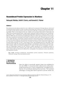
Fig. 11.2 The 7-DOF Mitsubishi PA-10 manipulator

Fig. 11.3 The 8-DOF DEXTER by Scienzia Machinale

Fig. 11.1 The 7-DOF DLR Lightweight Robot

1

Springer Handbook of Robotics Siciliano, Khatib (Eds.) · ©Springer 2008

task allows motions of the manipulator which do not displace the end effector (the so-called self-motions or internal motions); this implies that the same task at the

Kinematically Redundant Manipulators

robots often termed as human-arm-like manipulators. This family of 7-DOF manipulators includes the DLR Lightweight Robot (Fig. 11.1) and the Mitsubishi PA-10 robot (Fig. 11.2). An example of an 8-DOF robot is the DEXTER by Scienzia Machinale (Fig. 11.3). Manipulators with a larger number of joints are often called hyperredundant robots, and include many snake-like robots described in the literature. The use of two or more robotic structures to execute a task (as in the case of cooperating manipulators or multifingered hands) also gives rise to kinematic redundancy. Redundant mechanisms also include vehicle-manipulator systems; in this case, however, the possible presence of nonholonomic constraints on the motion of the base must be properly taken into account in order to determine the actual degree of redundancy. Although the realization of a kinematically redundant structure raises a number of issues from the point of view of mechanical design, this chapter focuses on redundancy resolution schemes, i. e., techniques for exploiting the redundant degrees of freedom in the solution of the inverse kinematics problem. This is an issue of major relevance for motion planning and control purposes.

11.2 Task-Oriented Kinematics The relationship between the variables representing the configuration of an articulated manipulator and those describing an assigned task in the appropriate space can be established at the position, velocity or acceleration level. In particular, consideration of the first-order task kinematics brings up the task Jacobian matrix, which is a central object in redundancy resolution techniques.

11.2.1 Task-Space Formulation A manipulator consists of a chain of rigid bodies articulated by joints. If qi denotes the variable characterizing the relative displacement of body i with respect to body i−1, the vector q = (q1 . . . q N ) uniquely describes the configuration of an N-joint serial-chain manipulator. Joint i may be either prismatic or revolute, in which case qi measures the relative translation or rotation of the attached links, respectively. While the manipulator is naturally described and actuated in the joint space, its operation is conveniently

specified in terms of the vector t = (t1 . . . t M ) , which typically defines the location of the manipulator endeffector in a suitably defined task space. In the general case, it is M=6 and t is chosen so that its first three components represent the position of the end effector, while its last three components represent a minimal description of the end-effector orientation (such as Euler angles or the roll–pitch–yaw representation), i. e., t = [ px p y Pz α β γ ] . Typically, one has N ≥ M, so that the joints can provide at least the number of degrees of freedom required for the end-effector task. If N > M strictly, the manipulator is kinematically redundant. The relationship between the joint-space coordinate vector q and the task-space coordinate vector t is expressed by the direct kinematics equation t = kt (q) ,

(11.1)

where kt is a nonlinear vector function. Springer Handbook of Robotics Siciliano, Khatib (Eds.) · ©Springer 2008

1

247

Part B 11.2

end-effector level can be executed in several ways at the joint level, giving the possibility of avoiding the forbidden regions and ultimately resulting in a more versatile mechanism. Such a feature is key to allowing operation in unstructured or dynamically varying environments that characterize advanced industrial applications and service robotics scenarios. In practice, if properly managed, the increased dexterity characterizing kinematically redundant manipulators may allow to avoid singularities, joint limits, and workspace obstacles, but also to minimize torque/energy over a given task, ultimately meaning that the robotic manipulator can achieve a higher degree of autonomy. The biological archetype of kinematically redundant manipulator is the human arm, which, not surprisingly, also inspires the terminology used to characterize the structure of serial-chain manipulators. In fact, the human arm has three degrees of freedom at the shoulder, one degree of freedom at the elbow and three degrees of freedom at the wrist. The available redundancy can be easily verified by locking one’s wrist, e.g., on a table and moving the elbow while keeping the shoulder still. The kinematic arrangement of the human arm has been replicated in a number of

11.2 Task-Oriented Kinematics

248

Part B

Robot Structures

Task Jacobian and Geometric Jacobian It is useful to consider the first-order differential kinematics [11.1]

˙t = J t (q) q˙ ,

(11.2)

Part B 11.2

that can be obtained by differentiating (11.1) with respect to time. In (11.2), ˙t is the task-space velocity vector, q˙ is the joint-space velocity vector, and Jt (q) = ∂kt /∂q is the M×N task Jacobian matrix (also called the analytic Jacobian). Remarkably, the components of t˙ relative to the endeffector orientation express the rate of change of the parameters characterizing the adopted minimal representation; they are not the components of the angular velocity vector of the end-effector. Indeed, denoting by v N the 3×1 translational velocity vector and by ω N the 3×1 angular velocity vector of the end-effector, and defining the end-effector spatial velocity v N as vN vN = (11.3) , ωN the following relationship holds ˙t = T(t) v N ,

(11.4)

where T is an M×6 transformation matrix that is a function of t only. In the case M =6, the transformation matrix T takes the form I 0 (11.5) T= , 0 R where I and 0 are, respectively, the identity and null matrix of proper dimensions, and R is a 3×3 matrix that specifically depends on the minimal representation used to describe the end-effector orientation. For a given manipulator, the mapping v N = J(q) q˙

(11.6)

relates a joint-space velocity to the corresponding endeffector velocity through the 6×N geometric Jacobian matrix J. The geometric Jacobian matrix is of major concern in the kinematic analysis of a manipulator since it allows description of the motion capabilities of the end-effector (in terms of its free rigid-body spatial velocity) as a result of the velocity commands at the joints in the current configuration. By comparing (11.2), (11.4), and (11.6), the relation between the geometric Jacobian and the task Jacobian can be found as J t (q) = T(t) J(q) .

1


(11.7)

Second-Order Differential Kinematics While the first-order differential kinematics (11.2) relates task-space to joint-space velocities, further differentiation with respect to time provides an analogous relationship between accelerations

¨t = J t (q)q¨ + J˙ t (q, q) ˙ q. ˙

(11.8)

This equation is also known as the second-order differential kinematics.

11.2.2 Singularities In this section the occurrence of singular configurations is considered to properly analyze their effect on inverse kinematics solutions. Representation and Kinematic Singularities A robot configuration q is singular if the task Jacobian matrix J t is rank-deficient there. Considering the role of J t in (11.2) and (11.8), it is easy to realize that at a singular configuration it is impossible to generate end-effector task velocities or accelerations in certain directions. Further insight can be gained by looking at (11.7), which indicates that a singularity may be due to a loss of rank of the transformation matrix T and/or of the geometric Jacobian matrix J. Rank deficiencies of T are only related to the mathematical relationship established by R between the angular velocity vector of the end-effector and the components of t˙ relative to the end-effector orientation; since the expression of R depends on the adopted minimal representation of the orientation, a configuration at which T is singular is then referred to as a representation singularity. Remarkably, any minimal description of the end-effector orientation experiences the occurrence of representation singularities. Furthermore, a given configuration may or may not yield a representation singularity depending on which description of orientation is used. A representation singularity is not directly related to the true motion capabilities of the manipulator structure, which can instead be inferred by the analysis of the geometric Jacobian matrix. Rank deficiencies of J are in fact related to loss of mobility of the manipulator endeffector; indeed, end-effector velocities exist in this case which are unfeasible for any velocity commanded at the joints. A configuration at which J is singular is referred to as a kinematic singularity. Since this chapter focuses on the inversion of the task differential kinematics (11.2) and (11.8), in the following the task Jacobian matrix and its singularities


(which include representation and kinematic singularities) are studied in detail. The case N ≥ M is considered, which encompasses conventional as well as redundant manipulators.

J t = UΣ V =

M

σi ui vi ,

(11.9)

i=1

where U is the M×M orthonormal matrix of the output singular vectors ui , V is the N×N orthonormal matrix of the input singular vectors vi , and Σ = (S 0) is the M×N matrix whose M×M diagonal submatrix S contains the singular values σi of the matrix J t . It is worth noticing that the SVD is a continuous and well-behaved function of its matrix argument; therefore, the input and output singular vectors as well as the singular values do not change much in the neighborhood of the current configuration. Letting rank (J t ) = R, the following hold:

•

σ1 ≥ σ2 ≥ . . . ≥ σ R > σ R+1 = · · · = 0;

•

R(J t ) = span{u1 , . . . , u R };

•

N (J t ) = span{v R+1 , . . . , v N }.

If the task Jacobian is full-rank (R= M), all the singular values are nonzero, the range space of J t is the entire R M , and the null space of J t has dimension N−M. In a singular configuration, instead, it is R< M; thus, the last M−R singular values are zero, the range space of J t is an R-dimensional subspace of R M , and the dimension of the null space of J t increases to N−R. An interpretation of this from a kinematic viewpoint is presented in the following. Feasible Velocities. At each configuration, the range

space of J t is the set of task-space velocities that can

be obtained as a result of all possible joint-space velocities q; ˙ therefore, it constitutes the so-called subspace of feasible velocities for the end-effector task. A base of R(J t ) is given by the first R output singular vectors, which represent independent linear combinations of the single components of the task velocities. Accordingly, the effect of a singularity is to decrease the dimension of the range space of J t by eliminating a linear combination of task velocity components from the space of feasible velocities. Null-Space Velocities. At each configuration, the null space of J t is the set of joint-space velocities which yield zero task velocity; these are thus shortly called nullspace velocities. A base of N (J t ) is given by the N−R last input singular vectors, which represent independent linear combinations of the velocities at each joint. From this viewpoint, the effect of a singularity is to increase the dimension of the null space of J t by introducing a further independent linear combination of joint velocities which produces a zero task velocity. According to (11.2) and (11.9), a joint velocity along the i-th input singular vector results in a task velocity which lies along the i-th output singular vector:

∀ρ ∈ R q˙ = ρ vi

⇒

t = σi ρ ui .

Thus, the i-th singular value of J t can be viewed as a gain factor relating motion along the vi direction of the joint velocity space to the resulting motion along the ui direction of the task velocity space. When a singularity is approached, the R-th singular value σ R tends to zero and the task velocity produced by a fixed joint velocity along v R is decreased proportionally. At a singular configuration, the joint-space velocity along v R belongs to the null-space velocities and task velocities along u R become unfeasible for the manipulator. In the generic case, the joint-space velocity q˙ is an arbitrary linear combination of individual joint velocities with nonzero components along all the vi . Its effect can be analyzed by combining the single effects of the above components. Remarkably, the components of q˙ in the null space of J t produce a change in the configuration of the manipulator without affecting its task velocity. This can be exploited to achieve additional goals – such as obstacle or singularity avoidance – in addition to the realization of a desired task motion, and constitutes the core of redundancy resolution approaches. Distance from Singularities Clearly, the effect of a singularity is experienced not only at the singular configuration itself but also in its Springer Handbook of Robotics Siciliano, Khatib (Eds.) · ©Springer 2008

1

249

Part B 11.2

Singular Value Decomposition of the Jacobian To analyze the linear mapping (11.2), the singular value decomposition (SVD) of the Jacobian matrix is adopted; remarkably, this powerful numerical tool is the sole reliable method to compute the rank of a matrix and to study near-singular linear mappings. The classic Golub– Reinsch algorithm [11.2], which is the most efficient and numerically stable algorithm to compute the SVD of an arbitrary matrix, may however be computationally demanding in view of real-time applications. A faster algorithm that takes advantage of the nature of robotic matrix calculations has been proposed [11.3]; this makes it possible to improve real-time kinematic control techniques. The SVD of the task Jacobian matrix can be written in the form

11.2 Task-Oriented Kinematics

250

Part B

Robot Structures

Part B 11.3

neighborhood (see also Sect. 11.3.2). For this reason, it is important to be able to characterize the distance from singularities through suitable measures; these can then be exploited to counteract undesirable effects. Since each singularity is associated to a rank loss of J t , one conceptually simple possibility in the case of a square Jacobian matrix (M = N) is to compute its determinant. A generalization of this idea that works also for nonsquare Jacobians is the manipulability measure [11.4], defined as μ = |J t J t |. It can be recognized that the manipulability measure is equal to the product of the singular values of J t , i. e., μ=

M

σi ,

i=1

and thus its zeros coincide with the singularities. Another possible measure of distance from a singular configuration is the condition number of the Jacobian matrix [11.5], defined as σ1 . κ= σM The condition number has values ranging from 1, at configurations in which all the singular values are equal,

to ∞, at singular configurations. Note that when κ =1 all the singular values are equal and thus the end-effector has the same motion capability in all task space directions – i. e., the arm is at an isotropic configuration – whereas at a singularity it loses mobility in some task-space direction. An even more direct measure of the distance from singular configurations is the smallest singular value of the Jacobian matrix [11.5], i. e., σmin = σ M . A computationally light estimate of the smallest singular value can be obtained either via numerical methods [11.3, 6, 7] or based on a kinematic analysis of the robot structure [11.8]. It must be noted that the manipulability measure may remain constant even in the presence of significant variations of either the condition number or the smallest singular value of J t . On the other hand, since the smallest singular value changes more radically near singularities than the other singular values, it dominates there the behavior of the determinant and the condition number of the Jacobian matrix; therefore, the most effective measure of distance from singular configurations is the smallest singular value of J t [11.5].

11.3 Inverse Differential Kinematics In order to accomplish a task, a proper joint motion must be commanded to the manipulator; therefore, it is necessary to derive mathematical relations which allow to compute joint-space variables corresponding to the assigned task-space variables. This is the objective of the inverse kinematics problem. The inverse kinematics problem can be solved by inverting either the direct kinematics equation (11.1), the first-order differential kinematics (11.2) or the second-order differential kinematics (11.8). If the task is time-varying (i. e., if a desired trajectory t(t) is assigned), it is convenient to solve the differential kinematic relationships because these represent linear equations with the task Jacobian as the coefficient matrix [11.9].

11.3.1 The General Solution Under the assumption that the manipulator is kinematically redundant (i. e., M < N), the general solution of (11.2) or (11.8) can be expressed by resorting to the † pseudoinverse J t of the task Jacobian matrix [11.1, 10];

1


this is the unique matrix satisfying the Moore–Penrose conditions [11.11–13] †

Jt Jt Jt = Jt †

†

†

Jt Jt Jt = Jt †

†

(J t J t ) = J t J t † (J t J t )

=

† Jt Jt

(11.10)

.

If J t is low-rectangular and full-rank, its pseudoinverse can be computed as †

−1 . Jt = J t (J t J t )

(11.11)

If J t is square, expression (11.11) reduces to the standard inverse matrix. The general solution of (11.2) can be written as †

†

q˙ = J t t˙ + (I−J t J t ) q˙ 0 . †

(11.12)

Here, I−J t J t represents the orthogonal projection matrix in the null space of J t , and q˙ 0 is an arbitrary


† q˙ = J t t˙

(11.13)

provides the least-squares solution of (11.2) with minimum norm, and is known as the pseudoinverse solution. In terms of the inverse differential kinematics problem, the least-squares property quantifies the accuracy of the end-effector task realization, while the minimum norm property may be relevant for the feasibility of the joint-space velocities. As for the second-order kinematics (11.8), its leastsquares solutions can be expressed in the general form †

†

q¨ = J t (t¨ − J˙ t q) ˙ + (I−J t J t ) q¨ 0 ,

(11.14)

where q¨ 0 is an arbitrary joint-space acceleration. As above, choosing q¨ 0 = 0 in (11.14) gives the minimumnorm acceleration solution: †

q¨ = J t (t¨ − J˙ t q) ˙ .

(11.15)

11.3.2 Singularity Robustness We now investigate the kinematics aspects involved by the first-order inverse mappings (11.12) and (11.13) with respect to the handling of singularities. With reference to the SVD of J t in (11.9), let us consider the following † decomposition of the matrix J t † Jt

†

= VΣ U

R 1 = vi ui , σi

(11.16)

i=1

where, as above, R denotes the rank of the task Jacobian matrix. Analogously to (11.9), the following hold:

•

σ1 ≥ σ2 ≥ . . . ≥ σ R > σ R+1 = · · · = 0 ;

•

R(J t ) = N ⊥ (J t ) = span{v1 , . . . , v R } ;

•

N (J t ) = R⊥ (J t ) = span{u R+1 , . . . , u M } .

†

†

Notice that, if the Jacobian matrix is full-rank, the † range space of J t is an M-dimensional subspace of † N R and the null space of J t is trivial. In a singular † configuration (R< M), instead, the range space of J t N is an R-dimensional subspace of R , and an M−R† dimensional null space of J t exists. † The range space of J t is the set of joint-space velocities q˙ that can be obtained via the inverse kinematic mapping (11.13) as a result of all possible task velocities t˙. Since these q˙ belong to the orthogonal complement of the null space of J t , the pseudoinverse solution (11.13) satisfies the least-squares condition, as expected. † The null space of J t is the set of the task velocities t˙ which yield null joint-space velocity in the current configuration; these t˙, on the other hand, belong to the orthogonal complement of the space of feasible task velocities. Therefore, one effect of the pseudoinverse solution (11.13) is to filter out the unfeasible components of the commanded task velocity while allowing exact tracking of the feasible components; this is related to the minimum-norm property. If the assigned task velocity is aligned with ui , the corresponding joint-space velocity – computed via (11.13) – is obtained along vi modulated by the factor 1/σi . When a singularity is approached, the R-th singular value tends to zero and a fixed task velocity command along u R requires joint-space velocities along v R that grow unboundedly in proportion to the factor 1/σ R . At the singular configuration, the u R direction becomes unfeasible for the task variables and v R adds to the null-space velocities of the arm. According to the above, two main problems are inherently related to the basic inverse differential kinematics solution (11.13), namely:

• •

at near-singular configurations, excessive jointspace velocities may result, due to the component of t˙ along the direction which becomes unfeasible at the singularity; at the singular configuration, discontinuity of the joint-space solution is experienced if ˙t has a non-null unfeasible component.

The same is obviously true for the complete inverse solution (11.12). Both the above problems are of major concern for kinematic control of manipulators, where the computed joint-space velocities must actually be executed by the robot arm. This has motivated the development of modified inverse differential mappings, so as to enSpringer Handbook of Robotics Siciliano, Khatib (Eds.) · ©Springer 2008

1

251

Part B 11.3

joint-space velocity; the second part of the solution is therefore a null-space velocity. Equation (11.12) provides all least-squares solution to the end-effector task constraint (11.2), i. e., it minimizes t˙−Jq. ˙ In particular, if J t is low-rectangular and full-rank, all joint velocities in the form (11.12) exactly realize the assigned task velocity. By acting on q˙ 0 , one can still obtain different joint velocities that give the same end-effector task velocity; therefore, as will be discussed later in detail, the solution in the form (11.12) is typically used in the context of redundancy resolution. The particular solution obtained by setting q˙ 0 = 0 in (11.12)

11.3 Inverse Differential Kinematics

252

Part B

Robot Structures

Part B 11.3

sure proper behavior of the manipulator throughout its workspace. A reasonable approach is to preserve the mapping (11.13) far from singularities and to set up local modifications of it only inside a region enclosing the singular configuration; the definition of the region depends on a suitable measure of distance from the singularity, while the modified mapping must ensure feasible and continuous joint velocities. Modification of the Planned Trajectory One way to tackle the problem of singularities is to act at the planning level by either designing trajectories that avoid unavoidable singularities or assigning taskspace motion commands that are feasible to the robot arm. However, these solutions rely on perfect task planning and cannot be used in real-time sensory control applications, in which motion commands are generated online. Avoidance of singular configurations at the motion planning level is relatively simple when dealing with those naturally characterized in the task space such as the shoulder singularity of an anthropomorphic arm. However, this approach may result difficult for those singularities, like the wrist one, that may occur everywhere in the workspace. Another possibility is to perform a joint-space interpolation when the planned trajectory is close to a singularity [11.14]; nevertheless, this may cause large errors in tracking the originally assigned task-space motion. Acting in the task space, a method based on timescale transformation is presented in [11.15], which slows down the manipulator’s motion when a singularity is approached; this technique, however, fails at the singularity. Since a task-space robot control system must be able to guide the motion of the manipulator safely through singularities, considerable research effort has been instead devoted to the derivation of well-defined and continuous inverse kinematic mappings. Removal of Dependent Rows or Columns of the Jacobian Matrix The first requirement of solution (11.13) is the availability of a general algorithm to compute the pseudoinverse of J t also when the Jacobian is singular. Several techniques presented in the literature can be arranged in this framework; they consist either in removing the unfeasible end-effector reference components [11.16] or in using nonsingular blocks of the Jacobian matrix [11.10]. The main problem with this type of solution is the spec-

1


ification of the directions of unfeasible velocities in a systematic way and the need to have smooth transitions between the usual inverse kinematic algorithm and the algorithms used close to the singularities. A systematic procedure to compute the pseudoinverse of the Jacobian matrix can be devised by taking advantage of kinematic analysis of the manipulator structure since for typical manipulators it is possible to identify and describe classes of singular configurations in suitably defined link-fixed frames. The approach has been demonstrated for a six-degree-of-freedom elbow geometry in [11.17, 18]. As for the continuity of the solution across a singularity, it must be observed that, while the singular vectors change very little in the neighborhood of the singularity, the term 1 v M u M t˙ σM suddenly disappears from (11.16) when R becomes less than M at the singular configuration. One possibility to avoid this problem is to make u M t˙ ≈ 0 in the neighborhood of the singularity, which means avoiding commanding task velocities along the direction that becomes unfeasible at the singular configuration. Nevertheless, as anticipated Sect. 11.3.2, it is reasonable to apply this approach only for preplanned trajectories in relation to unavoidable singularities that are naturally characterized in the task space. Independently from the assigned t˙, continuity of the pseudoinverse solution can be ensured by treating the manipulator as singular in a suitably defined region around each singularity through a modified Jacobian J¯ t , so that M−R extra degrees of freedom are available [11.17–19]; these can be used without significantly affecting the end-effector velocity, because the modified Jacobian J¯ t approximates J t inside the region. The described approach is difficult to generalize for multiple singularities. For the typical anthropomorphic geometry of industrial manipulators, however, only the wrist singularity is of primary concern since it may occur everywhere in the workspace, while the elbow and shoulder singularities are naturally characterized in the task space and thus can be avoided during planning. Regularization/Damped Least-Squares Technique The use of the damped least-squares technique in the inverse differential kinematics problem has been


independently proposed in [11.9, 20]. The method corresponds to solving the equation 2 J ˙ t t˙ = (J t J t +λ I) q

(11.17)

2 −1 q˙ = J t (J t J t +λ I) t˙ , 2 −1 q˙ = (J t J t +λ I) J t t˙ .

(11.18) (11.19)

The computational load of (11.18) is lower than that of (11.19), since usually N ≥ M. In the remainder, we will refer to the damped least-squares solution as q˙ = J ∗t (q) ˙t ,

(11.20)

whenever explicit specification of the computation used is not essential. Solution (11.20) satisfies the condition (11.21) min t˙−J t q ˙ 2 + λ2 q ˙ 2 , q˙

which realizes a trade-off between the least-squares and the minimum-norm properties. Condition (11.21) implies consideration of accuracy and feasibility at the same time as choosing the joint-space velocity required to match the given t˙. In this regard it is essential to suitably select the value to be assigned to the damping factor: small values of λ give accurate solution but low robustness to the occurrence of singular and nearsingular configurations; high values of λ result in low tracking accuracy even when a feasible and accurate solution would be possible. In the framework of singular value decomposition, the solution (11.20) can be written as q˙ =

R i=1

σi vi ui t˙ . σi2 + λ2

(11.22)

Remarkably, we have

•

R(J ∗t ) = R(J t ) = N ⊥ (J t ) = span{v1 , . . . , v R } ,

•

N (J ∗t )=N (J t )=R⊥ (J t )=span{u R+1 , . . . , u M } .

†

†

†

Analogously to J t , if the Jacobian matrix is full-rank, the range space of J ∗t is an M-dimensional subspace of R N and the null space of J ∗t is trivial; in a singular configuration, instead, the range space of J ∗t is an Rdimensional subspace of R N , and an M−R-dimensional null space of J ∗t exists.

253

It is clear that, with respect to the pure least-squares solution (11.13), in (11.22) the components for which σi λ are little influenced by the damping factor, since in this case 1 σi ≈ . σi σi2 + λ2 On the other hand, when a singularity is approached, the smallest singular value tends to zero while the associated component of the solution is driven to zero by the factor σi /λ2 ; this progressively reduces the joint velocity required to achieve near-degenerate components of the commanded t˙. At the singularity, the solutions (11.20) and (11.13) behave identically as long as the remaining singular values are significantly larger than the damping factor. Remarkably, due to the damping factor, an upper bound of 1/(2λ) exists on the gain factor relating for each i the task velocity component along ui to the resulting joint velocity along vi ; this bound is reached when σi =λ. Selection of the Damping Factor. According to above,

the value selected for the damping factor establishes the closeness of the current configuration to a singularity; moreover, λ determines the degree of approximation introduced with respect to the pure least-squares solution given by the pseudoinverse. An optimal choice for λ requires consideration of the smallest non-null singular value experienced along the given trajectory and of the minimum damping needed to ensure feasible joint velocities. To achieve good performance in the entire manipulator’s workspace the use of a configuration-varying damping factor has been proposed [11.9]. The natural choice is to adjust λ as a function of some measure of distance from the singularity at the current configuration of the robot arm. Far from singular configurations feasible joint velocities are obtained; thus the accuracy requirement prevails and low damping must be used. Close to a singularity, task velocity commands along the unfeasible directions give large joint velocities and the accuracy requirement must be relaxed; in these cases, high damping is needed. A first proposal was to adjust the damping factor as a function of the manipulability measure [11.9]. Since a more effective measure of distance from singular configurations is the smallest singular value of the Jacobian matrix [11.5], its use has been considered later for building a variable damping factor. If an estimate σˆ M of the smallest singular value is available, the following choice for the damping factor Springer Handbook of Robotics Siciliano, Khatib (Eds.) · ©Springer 2008

1

Part B 11.3

in place of (11.2). Here, λ∈ R is the damping factor. It can be recognized that, when λ is zero, (11.17) and (11.2) become identical. The solution to (11.17) can be written in two equivalent forms:

11.3 Inverse Differential Kinematics

254

Part B

Robot Structures

can be adopted [11.21] ⎧ ⎪ ⎨0

2 λ = 2 2 ⎪ ⎩ 1 − σˆ M /ε λmax

where β provides the largest contribution to damping only along the N−K estimated null-space velocity components vˆ i . This can be also recognized from the expression

when σˆ M ≥ ε otherwise, (11.23)

Part B 11.3

which ensures continuity and good shaping of the solution. In (11.23), ε defines the size of the singular region, in which damping is used, and λmax sets the maximum value of the damping factor, which occurs just at the singularity. Numerical Filtering. As can be recognized from (11.22),

the damping factor affects the accuracy of the solution along each end-effector velocity component; however, the sole unfeasible direction is responsible for the loss of tracking ability. To overcome this problem, selective filtering of the end-effector velocity components was proposed in [11.6]. The method can be generalized as follows; if an estimate uˆ i of the output singular vector associated to the M−K smallest singular values – which give the components to become unfeasible – is available, the solution can be written in the form −1 M 2 2 J + λ I + β J t˙ , u u q˙ = J ˆ ˆ t t t i i

q˙ ≈

K i=1

R σi σi ˙ v u v u t˙ , t + i i 2 +λ2+β 2 i i σi2+λ2 σ i=K +1 i

(11.27)

in which again the approximation is due to the estimates vˆ i in (11.26). Also in this case a nonzero value of λ is kept to guarantee satisfactory conditioning of the mapping (11.26) even for incorrect estimates of the input singular vectors. Comparison of (11.27) with (11.25) shows that, in the case of accurate estimate of the singular vectors, the solutions (11.24) and (11.26) behave identically.

11.3.3 Joint Trajectory Reconstruction

When solving the inverse kinematics problem at the firstorder differential level, one obtains the joint velocity profile q(t) ˙ that corresponds to an assigned end-effector task velocity profile t˙(t); however, the robot motion controller needs reference position trajectories in addition to the velocity references for the joints. The reconstruci=K +1 tion of the joint-position profile from the joint-velocity (11.24) profile obtained from an end-effector task velocity prowhere β provides the largest contribution to damping file t˙(t) realizes a kinematic inversion that can be seen only along the unfeasible components. This can also be as an inverse kinematics algorithm. recognized from the expression If the joint-velocity profile were completely specified (e.g., by its analytical expression) the corresponding K R σi σi ˙ ˙ joint-position profile could be obtained from time inteq˙ ≈ v u t+ v u t, 2 +λ2 i i 2 +λ2+β 2 i i σ σ gration i i i=1 i=K +1 t

(11.25)

in which the approximation is due to the estimates uˆ i in (11.24). Notice that K ≤ R; nevertheless, a nonzero value of λ is kept to guarantee satisfactory conditioning of the mapping (11.24) even for incorrect estimates of the output singular vectors. Similarly, additional damping can be provided to the joint-space velocity components given by the input singular vectors associated to the smallest singular values, since they are close to become the null-space velocities [11.22]. The solution can be generalized in the form −1 N 2 2 v v J + λ I + β J q˙ = J ˆ ˆ t i t t t˙ , i i=K +1

(11.26)

1


q(τ) dτ . ˙

q(t) = q(t0 ) +

(11.28)

t0

Nevertheless, digital implementation of the robot control system makes it more likely that a discrete-time sequence of samples q˙ k of the computed joint velocities at the time instants tk will be available, i. e., q˙ k = q(t ˙ k) . For this reason, a discrete-time numerical approximation of the continuous-time integral (11.28) must be suitably devised. Accurate discrete-time approximations of a continuous-time integral usually require a trade-off between the complexity of the interpolating algorithm and the


qk = q0 +

k−1

q˙ h Δt ,

(11.29)

h=0

where Δt is the time step. Equation (11.29) is usually written in the more effective recursive form qk = qk−1 + q˙ k−1 Δt . Closed-Loop Inverse Kinematics (CLIK) No matter what kind of interpolation is used, the small though unavoidable error suffered at each numerical integration step accumulates, leading to long-term drifting

of the reconstructed profile from the exact joint-position profile. Another source of error affecting any integral reconstruction method is the possible uncertainty in the initial value of the joint position. Algorithmic solutions that overcome these problems are based on the use of a feedback correction term; these are termed closed-loop inverse kinematics (CLIK) algorithms [11.23]. Considering, e.g., the case of first-order kinematics, the joint velocity at the k-th time instant is computed as (compare with (11.12)) † q˙ k = J t (qk ) t˙k + K tk−kt (qk ) † (11.30) + I−J t (qk )J t (qk ) q˙ 0k , where K is a constant positive-definite gain matrix. Second-order CLIK algorithms are also available that solve for joint positions, velocities, and accelerations [11.24, 25]. The CLIK approach was originally proposed in [11.26] and [11.27] based on the Jacobian transpose in lieu of the pseudoinverse, which provides remarkable computational savings and provides inherent singularity handling capabilities [11.28].

11.4 Redundancy Resolution via Optimization For a kinematically redundant manipulator, the inverse kinematics problem admits an infinite number of solutions, so that a criterion to select one of them is needed. In this section we will consider the problem of redundancy resolution via optimization at the first-order differential kinematics level. Before discussing algorithmic schemes for computing joint velocities, we provide a short review of possible performance criteria.

11.4.1 Performance Criteria The availability of degrees of freedom in excess with respect to those strictly needed to execute a given task can be used to improve the value of performance criteria during the motion. These criteria may depend on the robot joint configuration only, or also involve velocities and/or accelerations. Among the additional objectives that can be pursued by defining a suitable criterion, the most important is probably singularity avoidance. In fact, one of the main reasons for introducing kinematic redundancy is to reduce the extension of the workspace region where the manipulator is necessarily a singular configuration (unavoidable singularities). A discussion of avoidable and unavoidable singularities in redundant manipula-

tors can be found in [11.29]. If the assigned end-effector task does not pass through unavoidable singularities, it is in principle always possible to compute a joint trajectory along which the task Jacobian J t is continuously full-rank. To this end, possible performance criteria are the configuration-dependent functions introduced in Sect. 11.2.2 that characterize the distance from singularities, i. e., the manipulability measure, the condition number, and the smallest singular value of J t . Maximizing (or keeping as large as possible) these functions during the motion is a reasonable plan in order to avoid singular configurations during the motion. Since kinematic inversion produces diverging joint velocities in the vicinity of singular configurations, a conceptually different possibility is to minimize the norm of the joint velocity generated by the redundancy resolution scheme. However, this approach guarantees singularity avoidance only if such a norm is minimized in an integral sense along the motion of the manipulator. Local minimization of the norm [11.10] does not lead to singularity avoidance in any practical sense [11.29]. Redundancy can be also used to keep the manipulator linkage away from undesired regions of the joint space, for example, mechanical joint limits that are typically present in robot manipulators may be avoided by Springer Handbook of Robotics Siciliano, Khatib (Eds.) · ©Springer 2008

1

255

Part B 11.4

length of the time step. In real-time applications, such as robot motion control, high-order interpolation results in large finite-time delay that degrade the dynamic performance of the control loop. This time delay can be reduced by suitably shortening the time step; however, if the time step is sufficiently short even a low-order interpolation may give acceptable accuracy of the numerical integration. The typical case is that of a first-order interpolation, e.g., an Euler forward rectangular rule that transforms the integral (11.28) into

11.4 Redundancy Resolution via Optimization

256

Part B

Robot Structures

minimizing the cost function [11.30] 2 N 1 qi − qi,mid H(q) = 2 qi,max − qi,min i=1

Part B 11.5

where [qi,min , qi,max ] is the available range for joint i and qi,mid is its midpoint. Another interesting application is obstacle avoidance, which can be enforced by minimizing suitable artificial potential functions defined on the basis of the image of the obstacle region in the configuration space [11.31, 32]. Many other performance criteria have been proposed in the literature; some of them are mentioned in Sects. 11.6 and 11.9.

11.4.2 Local Optimization The simplest form of local optimization is represented by the pseudoinverse solution (11.13), which provides the joint velocity with the minimum norm among those which realize the task constraint. Clearly, the joint movement generated by this locally optimal solution does not provide global velocity minimization along the whole manipulator motion. This means that, despite the local minimization of joint velocities, singularity avoidance is not guaranteed [11.29]. Another possibility is to use the general solution (11.12), choosing the arbitrary joint velocity q˙ 0 in the direction of the antigradient of a scalar configurationdependent performance criteria H(q) which must be minimized: (11.31) q˙ 0 = −k H ∇ H(q) , where k H is a scalar step size and ∇ H(q) denotes the gradient of H at the current joint configuration. This leads to the following redundancy resolution scheme [11.30] † † (11.32) q˙ = J t t˙ − k H (I−J t J t ) ∇ H(q) . Since its second term is the projection of the antigradient of H in the null space of the task Jacobian, the above expression is reminiscent of the projected gradient method for constrained minimization [11.33]. In particular, it can be shown [11.34] that the inverse kinematic solution (11.32) minimizes the complete quadratic function 1 L(q, q) ˙ = q˙ q˙ + k H q˙ ∇ H(q) 2

at the current configuration q. Thus, (11.32) represents a natural trade-off between the unconstrained local minimization of the performance criteria H (which would lead to choose q˙ = −k H ∇ H(q)) and the satisfaction of constraint (11.2) by a minimum-norm joint velocity. The choice of the step size k H is critical for the performance of the redundancy resolution scheme (11.32). In particular, a small value of the step size may slow down the minimization of the performance criteria, but on the other hand a large value may even lead to an increase of H (recall that the antigradient is the local direction of maximum decrease). In practice, to identify at each configuration an appropriate value of k H in a reasonable time, one may use a simplified line search technique such as Armijo’s rule [11.33].

11.4.3 Global Optimization The main advantage of the redundancy resolution scheme (11.32) is its simplicity: if the computation of ∇ H(q) and k H is efficient, such a scheme is a realistic option for real-time kinematic inversion. Its disadvantage is to be found in the local nature of the optimization process, which can lead to unsatisfactory performance over long tasks, for example, use of (11.32) with H = −μ (the manipulability measure) will perform better than the simple pseudoinverse solution, but still cannot guarantee singularity avoidance. It is therefore natural to consider the possibility of selecting q˙ 0 in (11.12) so as to minimize integral criteria of the form tf H(q) dt ti

defined over the duration [ti , tf ] of the whole task (e.g., the integral manipulability along the motion). Unfortunately, the solution of this problem (naturally formulated within the framework of calculus of variations) may not exist, and in any case it admits no closed form in general. Remarkably, one way to make the problem certainly solvable is to include under the integral a quadratic form in the joint velocities or accelerations. However, this is more easily done at the second-order kinematic level (see Sect. 11.6).

11.5 Redundancy Resolution via Task Augmentation Another approach to redundancy resolution consists in augmenting the task vector so as to tackle ad-

1


ditional objectives expressed as constraints. In this section, we review the basic task augmentation tech-


niques for solving the first-order differential kinematics (11.2).

11.5.1 Extended Jacobian

†

N Jt = I − J t J t . It can be recognized that, for a given t0 , if q0 is a configuration at which the function g(q) is at an extreme under the constraint t0 =kt (q0 ), one has ∂g(q) N Jt (q0 ) = 0 . (11.33) ∂q q=q0 If the Jacobian J t has full rank M, then N Jt has rank N−M; therefore, equation (11.33) yields a set of N−M independent constraints that can be written in vector form as h(q) = 0 ; for example, these can be obtained by taking the scalar product of the gradient ∂g(q)/∂q by each of the N− M vectors constituting a base of the null space of J t , i. e., ∂g(q) . v M+1 (q) . . . v N (q) h(q) = ∂q At this point, the condition (11.33) implies that the equation

kt (q0 ) h(q0 )

=

t0 0

is satisfied. For motion starting from t0 with q0 that tracks a trajectory t(t) by keeping g(q) extremized at each time one has t(t) kt q(t) . = h q(t) 0

257

By differentiating both sides with respect to time one obtains ⎞ ⎛ J t (q) t˙ ⎟ ⎜ , (11.34) ⎝ ∂h(q) ⎠ q˙ = 0 ∂q where the matrix premultiplying the vector q˙ is square and is called the extended Jacobian J ext . Therefore, if the initial configuration q0 extremizes g(q) and provided that J ext does not become singular, the time integral of the inverse mapping t˙ (q) (11.35) q˙ = J −1 ext 0 tracks the assigned end-effector trajectory t˙(t) propagating joint configurations that extremize g(q). The extended Jacobian method has a major advantage over pseudoinverse techniques of the form (11.13) in that it is cyclic (see Sect. 11.7). Moreover, solution (11.35) can be made equivalent to (11.12) via suitable choice of the vector q˙ 0 [11.35, 37].

11.5.2 Augmented Jacobian Another approach, the so-called task-space augmentation, introduces a constraint task to be fulfilled along with the end-effector task; then, an augmented Jacobian matrix is set-up whose inverse gives the sought joint velocity solution. The concept of task-space augmentation has been independently introduced by Sciavicco and Siciliano [11.28, 38, 39] and Egeland [11.40] and later revisited by Seraji in the framework of the configuration control method [11.41]. In detail, let us consider the vector tc = (tc,1 . . . tc,P ) which describes the additional tasks to be fulfilled besides the M-dimensional end-effector task t. In the general case P ≤ N−M, although full redundancy exploitation suggests the consideration of exactly as many additional tasks as the number of redundant degrees of freedom, i. e., P = N−M. The relation between the joint-space coordinate vector q and the constraint-task vector tc can be considered as a direct kinematics equation tc = kc (q) ,

(11.36)

where kc is a continuous nonlinear vector function. Accordingly, it is useful to consider the mapping ˙tc = J c (q) q˙ ,

(11.37) Springer Handbook of Robotics Siciliano, Khatib (Eds.) · ©Springer 2008

1

Part B 11.5

The extended Jacobian technique, proposed by Baillieul [11.35] and later revisited by Chang [11.36], enforces an appropriate number of functional constraints to be fulfilled along with the original end-effector task so as to identify a single solution among the infinite compatible with the end-effector task. Let us consider an objective function g(q) to be optimized and let also N Jt (q) be a matrix spanning the null space of J t at a nonsingular configuration q, e.g.,

11.5 Redundancy Resolution via Task Augmentation

258

Part B

Robot Structures

Part B 11.5

that can be obtained by differentiating Eq. (11.36). In (11.37), t˙c is the constraint-task velocity vector, and J c (q) = ∂kc /∂q is the P×N constraint-task Jacobian matrix. At this point, an augmented-task vector can be defined by stacking the end-effector task vector with the constraint-task vector as kt (q) t = . ta = tc kc (q) According to this definition, finding a joint configuration q that results in some desired value for ta means satisfying both the end-effector and the constraint task at the same time. A solution to this problem can be found at the differential level by inverting the mapping ˙ta = J a (q) q˙

(11.38)

in which the matrix Jt Ja = Jc is termed the augmented Jacobian. A particular choice for the constraint-task vector is tc =h(q), with h defined as explained in Sect. 11.5.1, which allows the augmented Jacobian method to embed the extended Jacobian one.

11.5.3 Algorithmic Singularities The definition of additional goals besides tracking the end-effector velocity raises the possibility that configurations exist at which the augmented kinematics problem is singular while the sole end-effector task kinematics is not; these configurations are then termed algorithmic singularities [11.35]. With reference to the velocity mappings (11.34) and (11.38), an algorithmically singular configuration is one at which, respectively, the extended and the augmented Jacobians are singular while J t is full-rank. Since the origin of task-augmentation redundancy resolution methods, Baillieul pointed out that algorithmic singularities are not a specific problem of the extended Jacobian technique but that they arise from the way in which the constraint task conflicts with the endeffector task [11.35, 37]. This is easily understandable in simple situations such as that of a trajectory tracking with obstacle avoidance problem: if the assigned trajectory passes through an obstacle either the trajectory is

1


tracked or the obstacle is avoided so that both tasks cannot be achieved. If the origin of the conflict between the two tasks has a clear meaning the algorithmic singularity may then be avoided by keenly specifying the constraint task case by case (e.g., [11.23]). In more general situations analytical tools may be useful in finding algorithmic singularities and guiding the choice of the constraint function [11.42] or in finding configurations that better harmonize the two tasks [11.43]. Looking at the tasks definitions in (11.2) and (11.37), by considering their inverse mappings it can be recognized that the two tasks are in conflict when (11.39) R J c ∩ R J t = {0} and then this is the condition for the occurrence of an algorithmic singularity. On the other hand, when R J c ∩ R J t = {0} the two tasks are compatible since the two inverse mappings are linearly independent; a special case of task compatibility is when ⊥ Jt R J (11.40) c ≡R and the two mappings are orthogonal. At the algorithmic singularities the augmented Jacobian cannot be inverted but singularity-robust techniques can be adopted. Since the exact solution does not exist there are reconstruction errors and these affect both the task vectors. To counteract this problem the use of weighted damped least-squares has been considered to invert the augmented Jacobian matrix [11.44,45]. A different approach is the so-called task priority inverse kinematics.

11.5.4 Task Priority Conflicts between the end-effector task and the constraint task are handled in the framework of the task-priority strategy by suitably assigning an order of priority to the given tasks and then satisfying the lowerpriority task only in the null space of the higher-priority task [11.46, 47]. In the typical case, an end-effector task is considered as the primary task, although examples might be given in which it becomes the secondary task [11.23]. The idea is that, when an exact solution does not exist, the reconstruction error should only affect the lower-priority task. With reference to solution (11.12), the task-priority method consists of computing q˙ 0 so as to suitably achieve the P-dimensional constraint-task velocity ˙tc .


q˙ 0 = J †c (q)t˙c

(11.41)

would easily solve the problem, being in addition already a null-space velocity for the primary-task velocity mapping (11.2) (i. e., projection through N Jt would not be needed). However, in the general case the two tasks may be compatible but not orthogonal or may conflict and there not exist a joint velocity solution that ensures the achievement of both t˙ and t˙c . Coherently with the defined order of priority between the two tasks, a reasonable choice is then to guarantee exact tracking of the primary-task velocity while minimizing the constraint-task velocity reconstruction error t˙c − J c q; ˙ this gives [11.49] † † † q˙ 0 = J c (I − J t J t ) (t˙c − J c J t t˙) . (11.42) Finally, by observing that the null-space projection operator is both hermitian and idempotent, the solution given by (11.12) and (11.42) can be simplified to [11.46] † † † † (11.43) q˙ = J t t˙ + J c (I − J t J t ) (t˙c − J c J t t˙) . It can be recognized that the problem of algorithmic singularities still remains; in fact, when † condition (11.39) is satisfied the matrix J c (I − J t J t ) loses rank with full-rank J t and J c . However, differently from the task-space augmentation approach, correct primary-task solutions are expected as long as the sole primary-task Jacobian matrix is full-rank. On the other hand, out of the algorithmic singularities the task-priority strategy gives the same solution as the taskspace augmentation approach; this implies that close

to an algorithmic singularity the solution becomes illconditioned and large joint velocities may result. This problem has partly been solved by looking at the efficient rank of the matrix involved and treating it as singular depending on a suitable threshold [11.46]; the obtained joint velocities are thus limited, but continuity of the null-space component must be ensured. Another approach is to relax minimization of the secondary-task velocity reconstruction constraint and simply pursue tracking of the components of (11.41) that do not conflict with the primary task [11.50, 51], namely †

†

q˙ = J t t˙ + (I − J t J t )J †c t˙c .

(11.44)

An intuitive justification of this solution can be given as † † follows: The pseudoinverses J t and J c are used to solve separately for the joint velocities associated with the respective task velocities; the joint velocity associated with the (secondary) constraint task is then projected onto the null space of J t to remove the components that would interfere with the (primary) end-effector task and finally added to the joint velocity associated with the end-effector task. As a result, a nice property of solution (11.44) is that algorithmic singularities are decoupled from the singularities of J c . By construction, the solution (11.44) leads to larger constraint-task reconstruction errors than solution (11.43); this is the price paid to give smooth and feasible trajectories for the joint velocity in tracking conflicting tasks. Nevertheless, solution (11.44) is better used in a CLIK implementation which allows to recover the secondary-task tracking error out of the algorithmic singularities. In this case, it becomes †

†

q˙ = J t wt + (I − J t J t )J †c wc with

wt = t˙ + K t t−kt (q) wc = t˙c + K c tc−kc (q) .

11.6 Second-Order Redundancy Resolution Redundancy resolution at the acceleration level allows the consideration of dynamic performance along the manipulator motion. Moreover, the obtained acceleration profiles can be directly used as reference signals (together with the corresponding positions and velocities) of a task-space dynamic controller. On the other hand, a second-order redundancy resolution scheme is

invariably more demanding in terms of computational load. The simplest scheme operating at the acceleration level is represented by (11.15), i. e., the solution with the minimum norm among those which realize the task constraint (11.8). Similarly to the velocity-level pseudoinverse solution, the joint movement generated by Springer Handbook of Robotics Siciliano, Khatib (Eds.) · ©Springer 2008

1

259

Part B 11.6

Remarkably, the projection of q˙ 0 onto the null space of Jt ensures lower priority of the constraint task with respect to the end-effector task since this results in a null-space velocity for it [11.48]. When the secondary task t˙c is orthogonal to the primary task t˙ (in the sense of Eq. (11.40)) the joint velocity

11.6 Second-Order Redundancy Resolution

260

Part B

Robot Structures

this locally optimal solution does not provide global acceleration minimization along the whole manipulator motion. Remarkably, however, the use of (11.15) leads to the minimization over [ti , tf ] of the integral index tf

q˙ q˙ dt ,

Part B 11.7

ti

provided that the appropriate boundary conditions are satisfied [11.52], for example, in the case of free endpoints (neither joint positions nor velocities specified at ti and tf ) the boundary conditions to be satisfied are split and expressed as † q( ˙ t¯ ) = J t t˙(t¯ )

t¯ = ti , tf .

In spite of the apparent simplicity and elegance of the solution (11.15), therefore, actual minimization of the above integral cost requires the solution of a two-point boundary value problem (TPBVP), which is a computationally intensive numerical procedure impractical for real-time kinematic control. However, this may be perfectly acceptable for offline redundancy resolution in an industrial setting. More flexibility in the choice of (both local and global) performance criteria is obviously obtained by considering the full second-order solution (11.14). Let the manipulator dynamic model be expressed as τ = H(q)q¨ + c(q, q) ˙ + τg (q) ,

with †

τ˜ = H J t (t¨ − J˙ t q) ˙ + c + τg . leads to the local minimization of the actuator torque norm τ τ [11.53]. This particular redundancy resolution scheme performs reasonably over short tasks, but may lead to instability (more precisely, very high joint torques) in the long run, essentially due to the build-up of null-space joint velocities. Note also that the matrix † product H(I − J t J t ) in (11.46) is not full-rank, so that its pseudoinverse must be computed through a SVD procedure. Minimization of the integral joint torque is also possible [11.54]; this solution obviously avoids the instability problem, but once again the solution of a TPBVP is required. Another interesting inverse solution is the following † † q¨ = J t,H (t¨ − J˙ t q) ˙ + (I−J t,H J t ) H−1 c ,

which is slightly modified with respect to the general formula (11.14) in view of the use of a weighted pseu† doinverse. In particular, J t,H is the inertia-weighted task Jacobian pseudoinverse, given in the full-rank case by the following expression †

−1 −1 Jt ) . J t,H = H−1 J t (J t H

The solution (11.47) minimizes tf

(11.45)

where τ is the vector of actuator torques, H is the manipulator inertia matrix, c is the vector of centrifugal/Coriolis terms, and τg is the gravitational torque vector. Choosing the null-space acceleration in (11.14) as † † (11.46) q¨ 0 = − H(I − J t J t ) τ˜ ,

(11.47)

1 q˙ H(q)q˙ dt , 2

ti

i. e., the integral over [ti , tf ] of the manipulator kinetic energy [11.52]. Once again, the correct boundary conditions must be used; for example, the case of free endpoints leads to †

q( ˙ t¯ ) = J t,H ˙t (t¯ )

t¯ = ti , tf .

11.7 Cyclicity A common drawback of redundancy resolution schemes based on differential kinematics is the lack of cyclicity (also called repeatability): in general, the joint-space trajectory corresponding to a cyclic task space trajectory is not cyclic itself (i. e., the final position of the joints does not coincide with the initial position). This phenomenon is clearly undesirable, because it basically means that the behavior of the manipulator along periodic tasks to be repeated over and over is unpredictable.

1


A mathematical condition for cyclicity exists for a particular class of redundancy resolution methods [11.55]. In particular, consider any scheme of the form q˙ = G t (q)t˙ ,

(11.48)

where G t is any generalized inverse of the task Jacobian J t , i. e., an N × M matrix such that J t G t J t = J t † (the pseudoinverse matrix J t in (11.13) is a particular


generalized inverse). Assume that the assigned task t(t) describes a cyclic trajectory in a simply connected region of the task space, and denote by gti (q) the i-th column of G t . A necessary and sufficient condition for (11.48) to generate cyclic joint trajectories is that the distribution ΔG t (q) = span{gt1 (q), . . . , gtM (q)}

for cyclicity depends on the chosen generalized inverse (i. e., pseudoinverse, weighted pseudoinverse, and so on) as well as on the form of J t , which in turn is related to the mechanical structure of the manipulator. This means that cyclicity must be established on a case-by-case basis. As for redundancy resolution schemes which do not fall in the class (11.48) – namely, those entailed by the general inverse solution (11.12) – they are in general not cyclic. In particular, this is true for when local optimization is used to solve redundancy, as in (11.32). A notable exception is the extended Jacobian method, which is always cyclic.

11.8 Hyperredundant Manipulators A natural question arising from consideration of kinematic redundancy is: what happens as the number of joints (and hence degree of redundancy) becomes much larger than the task-space dimension, and ultimately increases towards infinity? Examples of serial rigid-link systems with many joints exist in nature (snakes, and mammalian and fish backbones, for example), and these biological existence proofs have provided motivation and insight for robot analysts and hardware designers for many years. This interest has resulted in the development of several special sub-classes of redundant manipulators, collectively known as hyperredundant manipulators. This section reviews the underlying issues and state of the art in this interesting area. A manipulator is generally considered to be hyperredundant if its controllable configuration (joint) space degrees of freedom are comparable to, or exceed, its task space degrees of freedom. (Hence, seven- or eightDOF spatial rigid-link manipulators are not usually considered to be hyperredundant.) Hyperredundant manipulators have enhanced potential to use their extra joints for whole arm grasping/manipulation and maneuvering within tight obstacle fields. Their anticipated applications therefore include operations in congested environments (disaster relief, medical applications, etc.). Since as we have seen the addition of (any) redundant degrees of freedom adds fundamentally new capabilities (self-motion, subtask performance capability), intuitively it would seem that the addition of abundant degrees of freedom would enable (and demand from motion planners) increasingly novel and sophisticated behaviors. However, on closer observation, many of the motivating biological hyperredundant systems actu-

ally perform relatively restricted movements, controlled by very simple algorithms. For example, (biological) snake backbones have very many joints, yet snake movement is typically restricted to approximately sinusoidal motions, governed by simple parameters (amplitude, frequency). Therefore there are some key simplifications which designers and algorithm developers have sought and made use of in the development of hyperredundant manipulators, as discussed in Sect. 11.8.3. In terms of hardware development, the field has evolved in two major directions: vertebrate-like rigid-link designs, and invertebrate-like continuum manipulators. Summaries of the history and state of the art of each of these areas are given in the following two subsections. This is followed by a discussion of the unique analysis techniques required of and developed for hyperredundant robot systems. In all cases, the key issue is that of handling complexity, in one form or another.

11.8.1 Rigid-Link Hyperredundant Designs This category of hyperredundant manipulators is perhaps the most natural, in terms of being the logical evolution from traditional serial rigid link manipulators (redundant or not). Designs in this category feature a hyperabundance of joints in their (usually serial) rigid-link structure. A good early example of this class of manipulator hardware is the JPL Serpentine Robot [11.56], which featured 12 degrees of freedom in a modular design. The general trend has to shrink the size of the links, so that the robot structure resembles that of a biologSpringer Handbook of Robotics Siciliano, Khatib (Eds.) · ©Springer 2008

1

261

Part B 11.8

is involutive (i. e., it is closed under the Lie bracket operation). It should be emphasized that the involutivity of ΔG t is a strong condition, because it must be satisfied at any configuration. This suggests that most generalized inverses are not cyclic. Note also that the above condition

11.8 Hyperredundant Manipulators

262

Part B

Robot Structures

Part B 11.8 Fig. 11.5 The NASA special-purpose dextrous manipulator (SPDM) (courtesy MDA Federal)

Fig. 11.4 17-DOF robot (courtesy Robotics Research Cor-

poration)

ical backbone. This approach conceptually allows the development of manipulators with a very high degree of redundancy; for example, the 30-DOF planar manipulator developed at Caltech [11.57] remains perhaps the best known hyperredundant manipulator. Note that various types of nontraditional rigid-link based manipulator systems can be classified as hyperredundant systems within this category. A novel elephant’s trunk was based on a design featuring a 32-DOF backbone [11.58]. Several dual-arm/torso designs [11.59] including NASA’s special-purpose dextrous manipulator (SPDM) [11.60] can be grouped in this category of hyperredundant manipulators, and researchers in the area of humanoid robots have made contributions to the area, both in terms of theory and hardware. Another important special group in this category is that of robotic snakes. This area owes much to the pioneering work of Hirose [11.61], who analyzed the movements of (biological) snakes and incorporated the understanding generated into the design and control of a series of innovative snake-like robots. Of particular in-

1


Fig. 11.6 Active cord mechanism (courtesy S. Hirose)

terest here were the series of hyperredundant active cord mechanism (ACM) robots developed by Hirose’s group. Numerous other snake robot designs have been proposed over the years, and the area continues to be highly active. The key conceptual advantage of rigid-link hyperredundant designs is that they inherit the kinematics of their conventional industrial manipulator counterparts. Therefore, all the traditional modeling techniques (for example Denavit–Hartenberg-based approaches for modeling the forward kinematics and finding the manipulator Jacobian) apply. Therefore, in theory all the techniques discussed earlier in this chapter apply directly to this category of hyperredundant manipu-


11.8 Hyperredundant Manipulators

263

Part B 11.8

Fig. 11.7 The OctArm continuum manipulator (courtesy I. Walker)

lator (although complexity of the resulting models is a key obstacle to analysis and understanding). However, the second main category, overviewed in the following subsection, by taking hyperredundancy to its logical extreme, does not inherit these particular advantages.

11.8.2 Continuum Robot Designs The term continuum manipulator, first coined in [11.62], indicates the hyperredundant robot concept taken to the extreme. In other words, conceptually this category of robots have backbone structures taken to the limit, with their number of joints tending to infinity, but with their link lengths tending to zero. While this concept initially appears idealistic, complicated, and impossible to implement, the limiting case (a smooth continuum curve, with the ability to bend at any point along the backbone) is quite easy to realize in hardware. Numerous continuum designs have been proposed since the early 1960s [11.62, 63]. The key design issues revolve around how to actuate (bend and possibly extend/contract) the backbone. Two basic design strategies have emerged: (1) extrinsic actuation, where the actuators are separate from the backbone structure [11.64]; and (2) intrinsic actuation, where the actuators represent a fundamental part of the backbone, e.g., [11.65]. Tendons have proved a popular and generally successful choice for intrinsically actuated continuum designs [11.58,64]. Artificial muscle technologies, notably McKibben muscles, have proved effective in intrinsically actuated hardware realizations [11.65]. A commercially successful group of extrinsically actuated continuum manipulators are currently manu-

Fig. 11.8 The continuum manipulator (courtesy OC Robotics)

factured and retailed by OCR Robotics in the United Kingdom [11.64]. While continuum manipulators are thus seen to be the extreme case of hyperredundancy, it was quickly realized that they represent a fundamentally new class of manipulators [11.62]. A continuous flexible backbone features, at least in theory, an infinite number of degrees of freedom. As such, the traditional tools in robotics for modeling (a finite number of) serial rigid links no longer apply. Additionally, it is obviously not possible to actuate an infinite number of degrees of freedom in practice. Continuum manipulator hardware universally features a finite number of actuators, applying forces/torques to the backbone at a fixed and preselected set of locations. Continuum robots are therefore inherently both hyperredundant and underactuated. This causes significant complexity in their analysis. However, significant progress has been made, and understanding resulting from analysis of continuum kinematics has been applied to the benefit of both continuum and noncontinuum hyperredundant manipulators, as discussed in the following subsection.


1

264

Part B

Robot Structures

11.8.3 Hyperredundant Manipulator Modeling

Part B 11.8

Clearly, to correctly model continuum manipulators, models based on continuous backbones are required. Interestingly, such models have also proved to be key theoretical resources in the motion planning of rigidlink hyperredundant systems. As noted earlier, in theory discrete-link hyperredundant manipulators can be modeled using (and their planning based on) traditional manipulator modeling techniques. However, it was quickly found that the computational complexity of such approaches made them difficult to implement, and the corresponding models hard to visualize. An alternative strategy (and a more successful one in practice) has been to adopt an approach based on continuum manipulator kinematics. In the following, we overview the recent development of continuum manipulator kinematics. We then discuss how the existence of both discrete-link and continuum models have enhanced motion planning for each category of hyperredundant system. The lack of distinct links in continuum systems makes the standard robot manipulator modeling strategy of a finite number of coordinate frames (each fixed in one link) inappropriate for their modeling. Instead, the natural approach is to model continuum kinematics via a frame that evolves along the backbone, parameterized by arc length s. Local motion of the backbone at point s is modeled in terms of the local frame. This strategy allows computation of forward kinematics, and the construction of continuum Jacobians, analogous to those for rigid-link systems [11.65, 66]. Numerous alternatives for selection of the backbone frame have been proposed [11.67,68]. A popular choice is the well-known Serret–Frenet frame [11.66], which evolves along the backbone according to: dt = κn , ds dn = −κt + τb , ds db = −τn . ds In the above, the frame origin is given by x, where the unit tangent to the curve t = dx/ ds, and forms one of the frame axes. The other axes are defined as the normal (t · n = 0) and the binormal b = t × n. The curvature κ and torsion τ dictate the shape of the curve. The axes of the Serret–Frenet frame provide an intuitive visualization of local movement: two possible dimensions of bending, corresponding to rotations

1


about the normal and binormal axes, and one of extension/contraction (present and controllable in several continuum robots), corresponding to translation along the tangent axis. The Frenet–Serret model has the advantage of being a well-established means for modeling continuous spatial curves. Alternative frame representations in the continuum robot literature have selected the axes of the frame to align with the controlled motion axes of particular hardware realizations [11.68]. In either case, given a frame, the key problem is how to use the resulting model to plan motions for hyperredundant robots. The basic issue is that the continuum kinematics models in their basic form feature infinite degrees of freedom (as necessary to model arbitrary spatial curves). However, hyperredundant robots (discrete-joint or continuum) can be controlled in only a finite number of ways, thus admitting a reduced set of physical solutions. Therefore, research in hyperredundant manipulators has concentrated on how to constrain continuum kinematics models to best represent robot hardware. The initial major breakthrough in motion planning for hyperredundant arms was made in a landmark series of papers [11.57, 67, 69] introducing continuum kinematics and using them to approximate rigid-link hyperredundant systems [11.67]. Basically the philosophy is to use a (theoretical) curve to model the physical backbone of a hyperredundant robot. Motion planning is performed for the curve, and the (discrete) robot backbone is then fitted to the resulting (continuous) solution curve. This approach has proved quite effective, and the associated research introduced several key theoretical concepts to the area. In particular, the use of a modal approach [11.69] (restricting the classes of allowable solutions to shapes generated via simple linear combinations of modes), arose from this approach to redundancy resolution for hyperredundant manipulators. This influential concept can be viewed as a top-down approach of building a general model, and adapting it (via mode selection and curve fitting) to hardware. More recent research has concentrated on the dual notion to that of the previous section, using the physical constraints imposed on the backbones of specific continuum robot hardware types to construct continuum kinematics. This can be viewed as a bottom-up approach, focused on particular hardware classes, with the main aim of sufficiently modeling the hardware to avoid the use of approximations in the motion planning. Examples of this approach are given in [11.65,68], where the key constraint imposed on a general continuum kinematics model arises from the observation that many continuum hardware implementations resolve into


resolution for rigid-link hyperredundant arms. Finally, a series of Jacobians are formed. The difference here is that the continuum Jacobian is a function of locally meaningful variables (bending angle, curvature, and extension) defining section shape or the direct values of the actuators that determine these variables. Given the existence of continuum Jacobians, the redundancy is usually resolved as † † I˙ = J E ˙tE + (I − J E J E ) I˙ 0

in the same way as for conventional redundant manipulators (and with the same general corresponding advantages and issues), as discussed earlier in the chapter.

11.9 Conclusion and Further Reading Research on kinematically redundant robots has been flourishing for over two decades now, and is still very active. The number of papers dealing with this subject is therefore enormous. The few works cited below are simply a small addition to the fundamental contributions already referenced so far, and constitute by no means an exhaustive list. The mechanical design of kinematically redundant manipulators has been studied in many papers, see, e.g., [11.70–74]. In particular, the superiority of humanarm-like manipulators over conventional 6-DOF robots was first advocated in [11.75]. Reconfiguration of this arm so as to ensure full mobility in the whole workspace is studied in [11.76, 77]. A general analysis of the inverse kinematic problem for redundant manipulators is presented in [11.78]. In particular, the geometric structure of self-motions is analyzed in [11.79]. Weighting the damped least-squares solution for guaranteed singularity avoidance in anisotropic endeffector tasks was proposed in [11.9, 21, 80].

In addition to singularity avoidance, redundancy has also been exploited to achieve obstacle avoidance [11.37, 46, 81, 82], minimization of the effects of joint elasticity [11.83], fault tolerance [11.84], reduction of impact force [11.85,86], and maximization of various dexterity measures [11.4, 5, 43, 87]. A completely different approach for obstacle avoidance with redundant robots is presented in [11.88]. A review of redundancy resolution via local optimization is given in [11.89]. A numerically efficient alternative for redundancy resolution via local optimization is proposed in [11.90]. A redundancy resolution approach with somehow intermediate characteristics between local and global optimization is presented in [11.91]. Other methods for second-order redundancy resolution are discussed, e.g., in [11.92]. Also worth citing is the dynamically consistent generalized inverse of [11.93]. The cyclicity issue was first pointed out in [11.94], and further investigated, e.g., in [11.95, 96]. General formalisms for redundancy resolution of vehiclemanipulator systems subject to nonholonomic constraints are described in [11.97, 98].

References 11.1

11.2

D.E. Whitney: Resolved motion rate control of manipulators and human prostheses, IEEE Trans. Man-Mach. Syst. 10(2), 47–53 (1969) G.H. Golub, C. Reinsch: Singular value decomposition and least-squares solutions, Numer. Math. 14, 403–420 (1970)

11.3

11.4

A.A. Maciejewski, C.A. Klein: The singular value decomposition: computation and applications to robotics, Int. J. Robot. Res. 8(6), 63–79 (1989) T. Yoshikawa: Manipulability of robotic mechanisms, Int. J. Robot. Res. 4(2), 3–9 (1985)


1

265

Part B 11

a finite number of constant curvature sections. (This arises naturally from the imposition of a finite number of input force/torques on a stiff continuum backbone.) In [11.65] it is noted that the resulting constant-curvature models can be viewed as a particular case of the general modal approach of [11.69]. The above approach [11.65] involves several transformations, to transition the map between task and actuator space via a section space. As a key part of this transformation, a conventional (theoretical) rigidlink model is used to model the kinematics of each section. Thus rigid-link kinematics have proven key to resolving redundancy for continuum manipulators, as continuum kinematics play a key part in redundancy

References

266

Part B

Robot Structures

11.5

11.6

Part B 11

11.7

11.8

11.9

11.10

11.11 11.12 11.13 11.14

11.15

11.16

11.17

11.18

11.19

11.20

11.21

11.22

1

C.A. Klein, B.E. Blaho: Dexterity measures for the design and control of kinematically redundant manipulators, Int. J. Robot. Res. 6(2), 72–83 (1987) A.A. Maciejewski, C.A. Klein: Numerical filtering for the operation of robotic manipulators through kinematically singular configurations, J. Robot. Syst. 5, 527–552 (1988) S. Chiaverini: Estimate of the two smallest singular values of the Jacobian matrix: application to damped least-squares inverse kinematics, J. Robot. Syst. 10, 991–1008 (1993) O. Egeland, M. Ebdrup, S. Chiaverini: Sensory control in singular configurations – application to visual servoing, IEEE Int. Workshop Intell. Motion Contr. (Istanbul 1990) pp. 401–405 Y. Nakamura, H. Hanafusa: Inverse kinematic solutions with singularity robustness for robot manipulator control, Trans. ASME – J. Dyn. Syst. Meas. Contr. 108, 163–171 (1986) D.E. Whitney: The mathematics of coordinated control of prosthetic arms and manipulators, Trans. ASME – J. Dyn. Syst. Meas. Contr. 94, 303–309 (1972) T.L. Boullion, P.L. Odell: Generalized Inverse Matrices (Wiley-Interscience, New York 1971) C.R. Rao, S.K. Mitra: Generalized Inverse of Matrices and its Applications (Wiley, New York 1971) A. Ben-Israel, T.N.E. Greville: Generalized Inverses: Theory and Applications (Wiley, New York 1974) R.H. Taylor: Planning and execution of straightline manipulator trajectories, IBM J. Res. Dev. 23, 424–436 (1979) M. Sampei, K. Furuta: Robot control in the neighborhood of singular points, IEEE J. Robot. Autom. 4, 303–309 (1988) E.W. Aboaf, R.P. Paul: Living with the singularity of robot wrists, IEEE Int. Conf. Robot. Autom. (Raleigh 1987) pp. 1713–1717 S. Chiaverini, O. Egeland: A solution to the singularity problem for six-joint manipulators, IEEE Int. Conf. Robot. Autom. (Cincinnati 1990) pp. 644–649 S. Chiaverini, O. Egeland: An efficient pseudoinverse solution to the inverse kinematic problem for six-joint manipulators, Model. Identif. Contr. 11(4), 201–222 (1990) O. Khatib: A unified approach for motion and force control of robot manipulators: the operational space formulation, IEEE J. Robot. Autom. 3, 43–53 (1987) C.W. Wampler II: Manipulator inverse kinematic solutions based on vector formulations and damped least-squares methods, IEEE Trans. Syst. Man Cybern. 16, 93–101 (1986) S. Chiaverini, O. Egeland, R.K. Kanestrøm: Achieving user-defined accuracy with damped leastsquares inverse kinematics, 5th Int. Conf. Adv. Robot. (’91 ICAR) (Pisa 1991) pp. 672–677 J.R. Sagli: Coordination of Motion in Manipulators with Redundant Degrees of Freedom. Ph.D. Thesis


11.23

11.24

11.25

11.26

11.27

11.28

11.29

11.30

11.31

11.32 11.33 11.34

11.35

11.36

11.37

11.38

11.39

(Institutt for Teknisk Kibernetikk, Norges Tekniske Høgskole, Trondheim, N 1991) P. Chiacchio, S. Chiaverini, L. Sciavicco, B. Siciliano: Closed-loop inverse kinematics schemes for constrained redundant manipulators with task space augmentation and task priority strategy, Int. J. Robot. Res. 10(4), 410–425 (1991) B. Siciliano: A closed-loop inverse kinematic scheme for on-line joint-based robot control, Robotica 8, 231–243 (1990) Z.R. Novaković, B. Siciliano: A new second-order inverse kinematics solution for redundant manipulators. In: Advances in Robot Kinematics, ed. by S. Stifter, J. Lenarˇciˇc (Springer-Verlag, Vienna, Austria 1991) pp. 408–415 A. Balestrino, G. De Maria, L. Sciavicco: Robust control of robotic manipulators, 9th IFAC World Congress (Budapest 1984) pp. 80–85 W.A. Wolovich, H. Elliott: A computational technique for inverse kinematics, 23rd IEEE Conf. Decis. Contr. (Las Vegas 1984) pp. 1359–1363 L. Sciavicco, B. Siciliano: A solution algorithm to the inverse kinematic problem for redundant manipulators, IEEE J. Robot. Autom. 4, 403–410 (1988) J. Baillieul, J. Hollerbach, R.W. Brockett: Programming and control of kinematically redundant manipulators, 23th IEEE Conf. Decis. Contr. (Las Vegas 1984) pp. 768–774 A. Liégeois: Automatic supervisory control of the configuration and behavior of multibody mechanisms, IEEE Trans. Syst. Man Cybern. 7, 868–871 (1977) O. Khatib: Real-time obstacle avoidance for manipulators and mobile robots, IEEE Int. Conf. Robot. Autom. (St. Louis 1985) pp. 500–505 J.C. Latombe: Robot Motion Planning (Kluwer Academic, Boston 1991) D.G. Luenberger: Linear and Nonlinear Programming (Addison-Wesley, Reading 1984) A. De Luca, G. Oriolo: Issues in acceleration resolution of robot redundancy, 3rd IFAC Symp. Robot Contr. (Vienna 1991) pp. 665–670 J. Baillieul: Kinematic programming alternatives for redundant manipulators, IEEE Int. Conf. Robot. Autom. (St. Louis 1985) pp. 722–728 P.H. Chang: A closed-form solution for inverse kinematics of robot manipulators with redundancy, IEEE J. Robot. Autom. 3, 393–403 (1987) J. Baillieul: Avoiding obstacles and resolving kinematic redundancy, IEEE Int. Conf. Robot. Autom. (San Francisco 1986) pp. 1698–1704 L. Sciavicco, B. Siciliano: Solving the inverse kinematic problem for robotic manipulators, 6th CISM-IFToMM Symp. Theory Practice Robots Manip. ´w 1986) pp. 107–114 (Krako L. Sciavicco, B. Siciliano: A dynamic solution to the inverse kinematic problem for redundant manipu-


11.40

11.41

11.43

11.44

11.45

11.46

11.47

11.48

11.49

11.50

11.51

11.52

11.53

11.54

11.55

11.56

11.57

11.58

11.59

11.60

11.61 11.62

11.63 11.64 11.65

11.66

11.67

11.68

11.69

11.70

11.71

11.72

11.73

11.74

E. Paljug, T. Ohm, S. Hayati: The JPL serpentine robot: a 12-DoF system for inspection, IEEE Int. Conf. Robot. Autom. (1995) pp. 3143–3148 G.S. Chirikjian, J.W. Burdick: Design and experiments with a 30 DoF robot, IEEE Int. Conf. Robot. Autom. (1993) pp. 113–117 M.W. Hannan, I.D. Walker: Kinematics and the implementation of an elephant’s trunk manipulator and other continuum style robots, J. Robot. Syst. 20(2), 45–63 (2003) J.P. Karlen, J.M. Thompson, H.I. Vold, J.D. Farrell, P.H. Eismann: A dual-arm dexterous manipulator system with anthropomorphic kinematics, IEEE Int. Conf. Robot. Autom. (1990) pp. 368–373 G. Hirzinger, B. Brunner, R. Lampariello, J. Schott, B.M. Steinmetz: Advances in orbital robotics, IEEE Int. Conf. Robot. Autom. (2000) pp. 898–907 S. Hirose: Biologically inspired robots (Oxford Univ. Press, Oxford 1993) G. Robinson, J.B.C. Davies: Continuum robots a state of the art, IEEE Int. Conf. Robot. Autom. (Detroit 1999) pp. 2849–2854 V.C. Anderson, R.C. Horn: Tensor arm manipulator design, Trans. ASME 67-DE-57, 1–12 (1967) R. Buckingham: Snake arm robots, Ind. Robot Int. J. 29(3), 242–245 (2002) B.A. Jones, I.D. Walker: Kinematics for multisection continuum robots, IEEE Trans. Robot. 22(1), 43–55 (2006) H. Mochiyama, E. Shimemura, H. Kobayashi: Shape correspondence between a spatial curve and a manipulator with hyper degrees of freedom, IEEE Int. Conf. Robot. Autom. (1998) pp. 161–166 G.S. Chrikjian: Theory and Applications of Hyperredundant Robotic Mechanisms. Ph.D. Thesis (Department of Applied Mechanics, California Institute of Technology 1992) I.A. Gravagne, I.D. Walker: Manipulability, force, and compliance analysis for planar continuum manipulators, IEEE Trans. Robot. Autom. 18(3), 263–273 (2002) G.S. Chirikjian, J.W. Burdick: A modal approach to hyper-redundant manipulator kinematics, IEEE Trans. Robot. Autom. 10(3), 343–354 (1994) J. Salisbury, J. Abramowitz: Design and control of a redundant mechanism for small motion, IEEE Int. Conf. Robot. Autom. (St. Louis 1985) pp. 323–328 J. Baillieul: Design of kinematically redundant mechanisms, 24th IEEE Conf. Decis. Contr. (Ft. Lauderdale 1985) pp. 18–21 G.S. Chirikjian, J.W. Burdick: Design and experiments with a 30 DoF robot, IEEE Int. Conf. Robot. Autom. (Atlanta 1993) pp. 113–119 J. Angeles: The design of isotropic manipulator architectures in the presence of redundancies, Int. J. Robot. Res. 11(3), 196–201 (1992) A. Bowling, O. Khatib: Design of macro/mini manipulators for optimal dynamic performance, Springer Handbook of Robotics Siciliano, Khatib (Eds.) · ©Springer 2008

1

267

Part B 11

11.42

lators, IEEE Int. Conf. Robot. Autom. (Raleigh 1987) pp. 1081–1087 O. Egeland: Task-space tracking with redundant manipulators, IEEE J. Robot. Autom. 3, 471–475 (1987) H. Seraji: Configuration control of redundant manipulators: theory and implementation, IEEE J. Robot. Autom. 5, 472–490 (1989) J. Baillieul: A constraint oriented approach to inverse problems for kinematically redundant manipulators, IEEE Int. Conf. Robot. Autom. (Raleigh 1987) pp. 1827–1833 S.L. Chiu: Control of redundant manipulators for task compatibility, IEEE Int. Conf. Robot. Autom. (Raleigh 1987) pp. 1718–1724 H. Seraji, R. Colbaugh: Improved configuration control for redundant robots, J. Robot. Syst. 7, 897–928 (1990) O. Egeland, J.R. Sagli, I. Spangelo, S. Chiaverini: A damped least-squares solution to redundancy resolution, IEEE Int. Conf. Robot. Autom. (Sacramento 1991) pp. 945–950 A.A. Maciejewski, C.A. Klein: Obstacle avoidance for kinematically redundant manipulators in dynamically varying environments, Int. J. Robot. Res. 4(3), 109–117 (1985) Y. Nakamura, H. Hanafusa, T. Yoshikawa: Taskpriority based redundancy control of robot manipulators, Int. J. Robot. Res. 6(2), 3–15 (1987) H. Hanafusa, T. Yoshikawa, Y. Nakamura: Analysis and control of articulated robot arms with redundancy, IFAC 8th Triennal World Congress (Kyoto 1981) pp. 78–83 Y. Nakamura, H. Hanafusa: Task priority based redundancy control of robot manipulators. In: Robotics Research – The Second International Symposium, ed. by H. Hanafusa, H. Hinoue (MIT Press, Cambridge 1985) pp. 155–162 S. Chiaverini: Task-priority redundancy resolution with robustness to algorithmic singularities, 4th IFAC Symp. Robot Contr. (Capri 1994) pp. 393–399 S. Chiaverini: Singularity-robust task-priority redundancy resolution for real-time kinematic control of robot manipulators, IEEE Trans. Robot. Autom. 13, 398–410 (1997) K. Kazerounian, Z. Wang: Global versus local optimization in redundancy resolution of robotic manipulators, Int. J. Robot. Res. 7(5), 312 (1988) J.M. Hollerbach, K.C. Suh: Redundancy resolution of manipulators through torque optimization, IEEE J. Robot. Autom. 3, 308–316 (1987) J.M. Hollerbach, K.C. Suh: Local versus global torque optimization of redundant manipulators, IEEE Int. Conf. Robot. Autom. (Raleigh 1987) pp. 619–624 T. Shamir, Y. Yomdin: Repeatability of redundant manipulators: Mathematical solution of the problem, IEEE Trans. Autom. Contr. 33, 1004–1009 (1988)

References

268

Part B

Robot Structures

11.75

Part B 11

11.76

11.77

11.78

11.79

11.80

11.81

11.82

11.83

11.84

11.85

1

IEEE Int. Conf. Robot. Autom. (Albuquerqe 1997) pp. 449–454 J.M. Hollerbach: Optimum kinematic design for a seven degree of freedom manipulator. In: Robotics Research – The Second International Symposium, ed. by H. Hanafusa, H. Hinoue (MIT Press, Cambridge 1985) pp. 216–222 O. Egeland, J.R. Sagli, S. Hendseth, F. Wilhelmsen: Dynamic coordination in a manipulator with seven joints, IEEE Int. Conf. Robot. Autom. (Scottsdale 1989) pp. 125–130 S. Chiaverini, B. Siciliano, O. Egeland: Kinematic analysis and singularity avoidance for a sevenjoint manipulator, Am. Contr. Conf. (San Diego 1990) pp. 2300–2305 D.R. Baker, C.W. Wampler: On the inverse kinematics of redundant manipulators, Int. J. Robot. Res. 7(2), 3–21 (1988) J.W. Burdick: On the inverse kinematics of redundant manipulators: characterization of the self-motion manifolds, IEEE Int. Conf. Robot. Autom. (Scottsdale 1989) pp. 264–270 S. Chiaverini, O. Egeland, R.K. Kanestrøm: Weighted damped least-squares in kinematic control of robotic manipulators, Adv. Robot. 7, 201–218 (1993) M. Kirć anski, M. Vukobratović: Trajectory planning for redundant manipulators in presence of obstacles, 5th CISM-IFToMM Symp. Theors Pract. Robots Manip. (Udine 1984) pp. 43–58 C.A. Klein: Use of redundancy in the design of robotic systems. In: Robotics Research – The Second International Symposium, ed. by H. Hanafusa, H. Hinoue (MIT Press, Cambridge 1985) pp. 207–214 J. Baillieul: Kinematic redundancy and the control of robots with flexible components, IEEE Int. Conf. Robot. Autom. (Nice 1992) pp. 715–721 J.D. English, A.A. Maciejewski: Fault tolerance for kinematically redundant manipulators: anticipating free-swinging joint failures, 14, 566–575 (1998) I.D. Walker: The use of kinematic redundancy in reducing impact and contact effects in manipulation, IEEE Int. Conf. Robot. Autom. (Cincinnati 1990) pp. 434–439


11.86

11.87 11.88

11.89

11.90

11.91

11.92

11.93

11.94

11.95

11.96

11.97

11.98

M.W. Gertz, J.O. Kim, P.K. Khosla: Exploiting redundancy to reduce impact force, IEEE/RSJ Int. Workshop Intell. Robot. Syst. (Osaka 1991) pp. 179– 184 T. Yoshikawa: Dynamic manipulability of robot manipulators, J. Robot. Syst. 2(1), 113–124 (1985) G. Oriolo, M. Ottavi, M. Vendittelli: Probabilistic motion planning for redundant robots along given end-effector paths, IEEE/RSJ Int. Conf. Intell. Robot. Syst. (Lausanne 2002) pp. 1657–1662 D.N. Nenchev: Redundancy resolution through local optimization: a review, J. Robot. Syst. 6, 6 (1989) A. De Luca, G. Oriolo: The reduced gradient method for solving redundancy in robot arms, Robotersysteme 7(2), 117–122 (1991) S. Seereeram, J.T. Wen: A global approach to path planning for redundant manipulators, IEEE Trans. Robot. Autom. 11(1), 152–160 (1995) A. De Luca, G. Oriolo, B. Siciliano: Robot redundancy resolution at the acceleration level, Lab. Robot. Autom. 4(2), 97–106 (1992) O. Khatib: Inertial properties in robotics manipulation: an object-level framework, Int. J. Robot. Res. 14(1), 19–36 (1995) C.A. Klein, C.H. Huang: Review of pseudoinverse control for use with kinematically redundant manipulators, IEEE Trans. Syst. Man Cybern. 13, 245–250 (1983) R. Mukherjee: Design of holonomic loops for repeatability in redundant manipulators, IEEE Int. Conf. Robot. Autom. (Nagoya 1985) pp. 2785– 2790 A. De Luca, G. Oriolo: Nonholonomic behavior in redundant robots under kinematic control, IEEE Trans. Robot. Autom. 13(5), 776–782 (1997) B. Bayle, J.Y. Fourquet, M. Renaud: Manipulability of wheeled-mobile manipulators: application to motion generation, Int. J. Robot. Res. 22(7-8), 565–581 (2003) A. De Luca, G. Oriolo, P.R. Giordano: Kinematic modeling and redundancy resolution for nonholonomic mobile manipulators, IEEE Int. Conf. Robot. Autom. (Orlando 2006) pp. 1867–1873

Springer Handbook of Robotics: Chapter 11

Springer Handbook of Robotics: Chapter 11

Suggest Documents

Springer Handbook of Robotics: Chapter 23

Springer Handbook of Robotics: Chapter 28

Springer Handbook of Robotics: Chapter 30

Springer Handbook of Robotics

Handbook of Robotics Chapter 22-Range Sensors

Chapter 11 - Springer Link

Chapter 11 - Springer Link

Chapter 11 - Springer Link

Chapter 11 - Springer Link

Chapter 11 - Springer Link

Chapter 11 - Springer Link

Chapter 11 - Springer Link

Chapter 11 - Springer Link

Chapter 11 - Springer Link

Chapter 11 - Springer Link

Handbook of Robotics Chapter 40: Multiple Mobile Robot ... - CiteSeerX

Handbook of Robotics Chapter 59: Robot ... - (LASA) | EPFL

Springer Handbook of Nanotechnology: Chapter 32

Springer Handbook of Nanotechnology: Chapter 16

Springer Handbook of Crystal Growth: Chapter 16

Springer Handbook of Nanotechnology: Chapter 16

Springer Handbook of Nanotechnology: Chapter 3

Springer Handbook of Nanotechnology: Chapter 3 - MAE

Springer Handbook of Automation: Chapter 73