Spurious regression under deterministic and stochastic trends
Antonio E. Noriega1 Daniel Ventosa-Santaulària2 Escuela de Economia Universidad de Guanajuato
JEL Classification: C22 Keywords: Unit roots, Trend stationarity, Structural breaks, Spurious regression
Abstract This paper analyses the asymptotic and finite sample implications of a mixed nonstationary behavior among the dependent and explanatory variables in a linear spurious regression model. We study the cases when the nonstationarity in the dependent variable is deterministic (stochastic), while the nonstationarity in the explanatory variable is stochastic (deterministic). In particular, we derive the asymptotic distribution of statistics in a spurious regression equation when one variable follows a difference stationary process (a random walk with and without drift), while the other is characterized by deterministic nonstationarity (a linear trend model with and without structural breaks in the trend function). We find that the divergence rate is sensitive to the assumed mixture of nonstationarity in the data generating process, and the phenomenon of spurious regression itself, contrary to previous findings, depends on the presence of a linear trend in the regression equation. Simulation experiments and real data confirm our asymptotic results.
1 Corresponding author. Escuela de Economia, Universidad de Guanajuato. UCEA, Campus Marfil, Fracc. I, El Establo, Guanajuato, Gto. 36250, México. Phone and Fax +52(473)7352925, e-mail:
[email protected]. 2 Escuela de Economia, Universidad de Guanajuato., e-mail:
[email protected]
1
1
Introduction
It is well documented by now that the phenomenon of spurious regression is present under different forms of nonstationarity in the data generating process (DGP ). It has been shown that when the variables yt and xt are nonstationary, independent of each other, ordinary least squares applied to the regression model yt = α + δxt + ut have the following implications: 1) the estimator of δ (b δ) does not converge to its true value of zero, and 2) the t-statistic for testing the null hypothesis H0 : δ = 0 (teδ ) diverges, thus indicating the presence of an asymptotic spurious relationship between yt and xt . The rate at which teδ diverges depends on the type of nonstationarity present in the process generating yt and xt . In Phillips (1986), where a driftless random walk is assumed for both variables, the t-statistic is Op (T 1/2 ). For the case of a random walk with drift, Entorf (1997) shows that teδ diverges at rate T . More recently, Kim, Lee and Newbold (2004) (KLN henceforth) show that the phenomenon of spurious regression is still present even when the nonstationarity in individual series is of a deterministic nature: they find that, under a linear trend stationary assumption for both variables, the t-statistic is Op (T 3/2 ). Extending KLN’s results, Noriega and Ventosa-Santaulària (2005) (NVS hereafter), show that adding breaks in the DGP still generates the phenomenon of spurious regression, but at a reduced divergence rate; i.e. teδ is O(T 1/2 ) under either single or multiple breaks in each variable. In all these works, the implicit assumption is that both variables share the same type of nonstationarity, either stochastic (Phillips, Entorf), or deterministic (KLN, NVS).3 This paper analyses the implications of a mixed nonstationary behavior among the dependent and explanatory variables. We develop the asymptotic theory for the cases when the nonstationarity in yt is deterministic (stochastic), while the nonstationarity in xt is stochastic (deterministic). In particular, we derive the limit distribution of statistics in the above regression equation when the DGP has mixed forms of nonstationarity: one variable follows a difference stationary process (a random walk with and without drift), while the other is characterized by deterministic nonstationarity (a linear trend model with and without structural breaks in the trend function). Indeed, recent empirical studies show that macroeconomic time series differ in the nature of their nonstationary behavior. For instance, in a multi-country study with historical data on real per capita GDP, Perron (1992) finds that some series are well characterized as (broken) trend-stationary (I(0) around a linear trend, and I(0) around a linear trend with one structural break), while others 3 Some related papers share this same feature: Marmol (1995, 1996, 1998), Cappuccio and Lubian (1997), Granger et. al. (1998) and Tsay and Chung (1999).
2
follow a unit root process. For the U.S. economy, Perron (1997) finds that real, nominal and real per capita GNP, employment, industrial production, nominal wage, and the money stock, stochastic nonstationarity (a unit root) can be rejected in favor of deterministic nonstationarity (a model with one structural break in the trend function); on the other hand, the consumer price index, velocity, interest rate and GNP deflator follow an I(1) process. Similar results are reported in Lumsdaine and Papell (1997) (US data) and Mehl (2000) (Japanese data) when testing the null of a unit root against a deterministic nonstationary alternative with two structural breaks in the trend function. Noriega and de Alba (2001) also find mixed forms of nonstationarity (I(1) and I(0) with one break) using macro data under both classical and Bayesian approaches. Looking ahead to the results reported below, we find that the divergence rate is sensitive to the assumed mixture of nonstationarity in the DGP , and the phenomenon of spurious regression itself depends on the presence of a linear trend in the regression equation, and on the presence of structural breaks in the DGP . For instance, if the dependent variable is I(1) while the explanatory is I(0) without breaks, a spurious relationship will show up both asymptotically and in finite samples, unless a linear trend is included in the regression model. We show this using asymptotic theory, simulation experiments, and real (macro) data. The rest of the paper is organized as follows. Section 2 reports asymptotic results for spurious regression under mixed forms of nonstationarity. Section 3 deals with experimental and empirical results. Last section concludes.
2
Asymptotics for spurious regressions
In a simple regression equation, stochastic nonstationarity may be a feature of the dependent variable, while deterministic nonstationarity of the explanatory variable, or viceversa. Since this can not be known a priori, we consider both possibilities: the dependent variable follows a trend-stationary (T S) process, while the explanatory variable follows a difference stationary (DS) one, and viceversa. Under difference stationarity, we study the cases of a unit root process with and without a drift, while under trend-stationarity we study the cases of a linear trend with and without multiple structural breaks in both level and slope of trend. These four types of nonstationary behavior for economic time series have been found to be empirically relevant in the literature, as argued above. The following assumption summarizes the DGP s considered below for both the dependent and the explanatory variables. Assumption. The DGP s for {yt , xt }∞ t=1 are as follows: DGP A1
yt = µy + β y t + uyt xt = xt−1 + uxt = x0 + Sxt
DGP A2
yt = µy + β y t + uyt xt = µx + xt−1 + uxt = x0 + µx t + Sxt 3
DGP A3
PN y PMy yt = µy + i=1 θiy DUiyt + β y t + i=1 γ iy DTiyt + uyt xt = µx + xt−1 + uxt = x0 + µx t + Sxt
DGP B1
xt = µx + β x t + uxt yt = yt−1 + uyt = y0 + Syt
DGP B2
xt = µx + β x t + uxt yt = µy + yt−1 + uyt = y0 + µy t + Syt
DGP B3
PN x PMx xt = µx + i=1 θix DUixt + β x t + i=1 γ ix DTixt + uxt yt = µy + yt−1 + uyt = y0 + µy t + Syt
P where, for z = x, y, Szt = ti=1 uzi , z0 is an initial condition, uzt = φz uzt−1 + εzt , |φz | < 1, εzt are iid(0, σ 2z ) independent of each other, and DUizt , DTizt are dummy variables allowing changes in the trend’s level and slope respectively, that is, DUizt = 1(t > Tbiz ) and DTizt = (t − Tbiz )1(t > Tbiz ), where 1(·) is the indicator function, and Tbiz is the ith unknown date of the break in z. We denote the break fraction as λz = (Tbz /T ) ∈ (0, 1). We maintain the same structure for the innovations uyt and uxt as in KLN, although it can also be assumed that innovations obey the (general-level) conditions stated in Phillips (1986, p. 313). As will be shown below: 1) the relevant limiting expressions do not depend on initial conditions (z0 ), and 2) they depend on σ 2z only under DGP s i2, i = A, B. We begin by considering the following spurious ordinary least squares regression model: b1 + b δ 1 xt + u bt (1) yt = α
used as a vehicle for testing the null hypothesis H0 : δ 1 = 0. The following theorems collect the asymptotic behavior of the estimated parameters and associated t−statistics in model (1) when the dependent and explanatory variables have mixed forms of nonstationarity, according to the DGP s in the Assumption. Proofs and definitions for some of the objects in the next theorems are collected in the Appendix. Theorem 1A. Let yt and xt be generated according to the DGP Ai, i = 1, 2, 3, and denote the corresponding OLS estimates of α1 and δ 1 in (1) by α b 1A(i) and b δ 1A(i) . Then, as T → ∞: Case (1): DGP A1.
d 1 −1 a) T −1 α b 1A(1) → 2 β y N1 D1
d 1 b) T −1/2b δ 1A(1) → 2 β y N2x (σ x D1 ) ¡ ¢−1/2 R d c) T −1/2 tαe 1A(1) → N1 13 D2x Wx2
−1
4
d
d) T −1/2 teδ1A(1) →
√ −1/2 3N2x D2x
Case (2): DGP A2
β
d b 1A(2) → σ x µy N3x a) T −1/2 α x
b) b δ 1A(2) → p
βy µx
−1/2
d 1 c) T −1/2 tαe 1A(2) → 2 N3x D2x
d µx σx
d) T −1 teδ1A(2) →
(12D2x )
−1/2
Case (3): DGP A3 p
a) T −1 α b 1A(3) → 24V4y
p b) b δ 1A(3) → (β y + 24V5y )µ−1 x
−1/2
p
c) T −1/2 tαe 1A(3) → 12V4y G6y p
d) T −1/2 teδ1A(3) → (β y + 24V5y )(12G6y )−1/2 Theorem 1B. Let yt and xt be generated according to the DGP Bi, i = 1, 2, 3, and denote the corresponding OLS estimates of α1 and δ 1 in (1) by α b 1B(i) and b δ 1B(i) . Then, as T → ∞: Case (1): DGP B1.
d a) T −1 α b 1B(1) → −σ y N3y
d b) T 1/2b δ 1B(1) →
σy β x 6N2y
d c) T −1/2 tαe 1B(1) → −N3y (4D2y )−1/2 d √ −1/2 d) T −1/2 teδ1B(1) → 3N2y D2y
Case (2): DGP B2.
d a) T −1/2 α b 1B(2) → −σ y N3y p b) b δ 1B(2) →
µy βx
−1/2
d c) T −1/2 tαe 1B(2) → − 12 N3y D2y
d µy σy
d) T −1 teδ1B(2) →
(12D2y )
−1/2
5
Case (3): DGP B3. £ ¡1 ¢ ¤−1 p a) T −1 α b 1B(3) → µy (V2x − β x V4x ) 2β x 48 β x + V5x − 2V3x ¡1 ¢£ ¡1 ¢ ¤−1 p b) b δ 1B(3) → µy 24 β x + V5x 2β x 48 β x + V5x − 2V3x £¡ 1 ¢¡ 2 ¢¤−1/2 p 2 c) T −1/2 tαe 1B(3) → (V2x − β x V4x ) 12 V1x − V4x β x + β x G1x + G3x + 6G4x ¢£ ¡ 1 ¢¤−1/2 p ¡ 1 2 d) T −1/2 teδ1B(3) → 24 β x + V5x 3 12 V1x − V4x Parts b) of the theorems show that, for DGP i1, i = A, B, the (normalized) estimated spurious parameter either goes to infinity (DGP A1), or collapses to zero (DGP B1). For the rest, it converges to well defined limits. Parts d) show that the spurious regression phenomenon is present under all DGP s, but occurs at a faster rate under DGP i2, i = A, B, which correspond to the models studied by Nelson and Plosser (1982). More over, the limiting distribution of the t-statistic for the hypothesis H0 : δ = 0 is symmetrical across DGP s Aj, and Bj, j = 1, 2. We now consider the case of a (spurious) OLS regression which allows for a linear trend. As discussed in KLN (2003), when the trend components in the individual series are sufficiently large to be detected, the applied researcher will run the following regression b t+b yt = α b2 + β δ 2 xt + u bt 2
(2)
where yt and xt are generated from the DGP s in the Assumption. The next theorems present the relevant asymptotic results.
Theorem 2A. Let yt and xt be generated according to the DGP Ai, i = 1, 2, 3, and denote the corresponding OLS estimates of α2 , β 2 , and δ 2 in (2) by b b α b 2A(i) , β 2A(i) , and δ 2A(i) . Then, as T → ∞: Case (1): DGP A1. p
a) α b 2A(1) → µy
p b b) β 2A(1) → β y d c) T b δ 2A(1) →
σy −1 σ x N4x D2x
d d) T −1/2 tαe 2A(1) →
e) T −3/2 tβe
2A(1)
d
d →
µy σy βy σy
³
³
−1/2
f ) teδ2A(1) → N4x D2x
D2x D3
´1/2
D2x 12D1
´1/2
6
Case (2): DGP A2. p
a) α b 2A(2) → µy p b b) β 2A(2) → β y d c) T b δ 2A(2) →
σy −1 σ x N4x D2x
d d) T −1/2 tαe 2A(2) →
e) T −1 tβe
2A(2)
µy σy
³
D2x D3
β y σ x 1/2 µx σ y D2x
d →
d
´1/2
−1/2
f ) teδ2A(2) → N4x D2x
Case (3): DGP A3.
b) c)
d) e)
£1
¤ −1 − G1y N1 + G5y N3x D2x £ ¡ ¢ ¤ R R −1 d b T −1/2 β Wy + V5y rWy − G5y (σ x D2x ) 2A(3) → µx 24 V4y £ ¡ ¢¤ R R −1 d T −1/2b G5y − 24 V4y Wy + V5y rWy (σ x D2x ) δ 2A(3) → ¡1 ¢£ ¤−1/2 d T −1/2 tαe 2A(3) → D3 σ u(A3) 2 G2y D3 − G1y N1 + G5y N3x £ ¡ ¢ ¤£ ¤−1/2 R R d T −1/2 tβe → 24 V4y Wy + V5y rWy − G5y σ u(A3)
d a) T −1 α b 2A(3) →
2 G2y D3
2A(3)
¡ R R ¢¤ £ ¤−1/2 d £ f ) T −1/2 teδ2A(3) → G5y − 24 V4y Wy + V5y rWy σ u(A3)
Theorem 2B. Let yt and xt be generated according to the DGP Bi, i = 1, 2, 3, and denote the corresponding OLS estimates of α2 , β 2 , and δ 2 in (2) by b b α b 2B(i) , β 2B(i) , and δ 2B(i) , Then, as T → ∞: Case (1): DGP B1.
d a) T −1/2 α b 2B(1) → −σ y N3y
σy d b b) β 2B(1) → − σ x N4y β x d c) b δ 2B(1) →
σy σ x N4y
d d) T −1/2 tαe 2B(1) → −σx N3y
e) tβe
−1/2
2B(1)
d → −N4y D2y
d
£¡ 2 ¢ ¤−1/2 µx + 4σ 2x D2y
−1/2
f ) teδ2B(1) → N4y D2y
7
Case (2): DGP B2. d
a) T −1/2 α b 2B(2) → −σ y N3y d b b) β 2B(2) → µy − d c) b δ 2B(2) →
σy σ x N4y β x
σy σ x N4y
£ ¡ ¢¤−1/2 d d) T −1/2 tαe 2B(2) → −σx N3y D2y µ2x + 4σ 2x h i −1/2 d σ x µy e) tβe → σ y β − N4y D2y 2B(2)
x
d
−1/2
f ) teδ2B(2) → N4y D2y
Case (3): DGP B3.
¡ R R ¢ d a) T −1/2 α b 2B(3) → 24σ y V2x rWy − 2V1x Wy + V4x G5x G−1 6x p b b) β 2B(3) → µy
£ ¡ ¢ ¤ R R d c) T 1/2b σ y 24 V4x Wy + V5x rWy − G5x G−1 δ 2B(3) → 6x ¡ ¢ ¡ ¢−1 R R p d d) T −1/2 tαe 2B(3) → V2x rWy − 2V1x Wy + V4x G5x 2 σu(B3) V1x n ¡ £ ¤¢ o−1 d 1 2 1/2 e) T −1 tβe → µy G6x 24σ y σ u(B3) 4 (V3x − β x V5x ) − 12 βx 2B(3)
¡ ¢ ¤¡ ¢−1 R R d £ f ) T −1/2 teδ2B(3) → 24 V4x Wy + V5x rWy − G5x 48σu(B3)
Parts f ) of the theorems show that the spurious regression parameter tstatistic only diverges to infinity under structural breaks; otherwise, it has a well defined limit. Hence, a spurious relationship will be present only under DGP i3, i = A, B. Note that, as opposed to the case of no trend in the regression, the spurious regression coefficient (and its t-statistic) converges to the same distribution across DGP s ij, i = A, B; j = 1, 2. Table A1 in the Appendix presents a summary of results concerning orders in probability of relevant statistics.
3
Experimental and empirical results
We computed rejection rates of the t-statistic for testing the null hypotheses H0 : δ j = 0, j = 1, 2, in equations (1) and (2), respectively, using a 1.96 critical value (5% level) for a standard normal distribution. In order to asses the usefulness of our limit theory in finite samples, rejection rates were based on both the asymptotic formulae and simulated data, for samples of size T = 50, 100, 250, 500, 1000, 10000, under each one of the DGP s
8
in the Assumption. The value of the parameters in the DGP s are as follows4 : σ z = 1, φz = 0 (but see below), µz = 0, or 0.5, depending on the DGP containing a drift or not, β z = 0.03 if the DGP contains a nonzero slope, and, whenever breaks are present, Mz = 2 and γ i = 0.03, i = 1, ..., Mz , for z = x, y. Breaks occur at 10% and 30% of total data length. The number of replications is 10, 000. The simulation experiments reveal a remarkable agreement in rejection rates between analytical results and simulated ones, as shown in Table 1. The only discrepancy occurs for the multibreaks model with trend (DGP s i3, i = A, B), for T < 500. Results also indicate that the rejection rates for the cases of the model without trend can be very high, even for values of the sample size as small as 50. Hence, in these cases, the phenomenon of spurious regression is likely to be present also in small (empirically relevant) samples.
Sample size 50 100 250 500 1,000 10,000
Sample size 50 100 250 500 1,000 10,000
Table 1 Rejection Rates for teδ ; DGP s Aj, j = 1, 2, 3. DGP A1 DGP A2
DGP A3
no trend theo sim
trend theo sim
no trend theo sim
trend theo sim
no trend theo sim
trend theo sim
0.83 0.88 0.92 0.95 0.96 0.99
0.05 0.05 0.04 0.05 0.05 0.05
1.00 1.00 1.00 1.00 1.00 1.00
0.06 0.05 0.05 0.05 0.05 0.05
1.00 1.00 1.00 1.00 1.00 1.00
0.69 0.77 0.86 0.89 0.93 0.98
0.82 0.87 0.93 0.94 0.96 0.99
0.06 0.05 0.06 0.04 0.04 0.05
0.82 1.00 1.00 1.00 1.00 1.00
0.06 0.05 0.04 0.05 0.05 0.05
Rejection Rates for teδ ; DGP s Bj, j = 1, 2, 3. DGP B1 DGP B2
0.99 1.00 1.00 1.00 1.00 1.00
0.06 0.15 0.67 0.86 0.92 0.98
DGP B3
no trend theo sim
trend theo sim
no trend theo sim
trend theo sim
no trend theo sim
trend theo sim
0.83 0.87 0.92 0.95 0.96 0.99
0.05 0.05 0.04 0.05 0.05 0.05
1.00 1.00 1.00 1.00 1.00 1.00
0.04 0.05 0.05 0.05 0.05 0.05
1.00 1.00 1.00 1.00 1.00 1.00
0.69 0.78 0.86 0.90 0.92 0.98
0.45 0.81 0.91 0.94 0.96 0.99
0.06 0.05 0.05 0.05 0.05 0.05
0.82 1.00 1.00 1.00 1.00 1.00
0.05 0.05 0.05 0.05 0.05 0.05
0.99 1.00 1.00 1.00 1.00 1.00
Note: theo and sim stand for theoretical (based on the corresponding theorem), and simulated.
When including a linear trend in the regression model, however, rejection rates for DGP s ij, i = A, B; j = 1, 2 do fluctuate around the nominal level, for any sample size. Hence, assuming no breaks in the DGP , the inclusion of a linear 4 We experimented with different values of the parameters, location and number of breaks, and obtained very similar results.
9
0.06 0.16 0.67 0.85 0.92 0.97
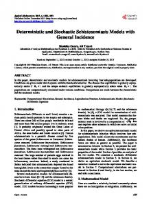
trend eliminates the spurious regression phenomenon, not only asymptotically, but also in finite samples. As can be seen from the theorems, the limiting distribution of teδ depends on σ 2z under DGP s i2, i = A, B. To asses the effect of autocorrelation, a simulation experiment was performed to compute rejection rates for DGP i2, i = A, B using φz = 0.1, 0.5, 0.9. Results revealed that rejection rates are greater that 60% even in the case of a sample as small as T = 50, and φz = 0.9. As the analytical results show, the presence of a linear trend in the regression equation ensures a well defined limit for the distribution of teδ2 , under DGP s ij, i = A, B; j = 1, 2. Figure 1 shows that this limit closely resembles a standard normal distribution. The Monte Carlo experiments used to generate the depicted densities were based on 1) A non-parametric estimation using 10,000 simulated data samples of 100 observations (labeled T = 100), under DGP B2, and regression equation (2), with parameter values: σ z = 1, φz = 0, µz = 0.5, β y = 0.03, for z = x, y; and 2) A non-parametric estimation using 30,000 replications and the asymptotic distributions of teδ2 (labeled Asymptotic), for DGP B2, as stated in Theorem 2B. Additionally, a standard normal distribution is included for comparison purposes.
Non-parametric estimation of teδ2 , for DGP B2.
To assess the empirical relevance of the above results, we utilize long, low frequency data of (log) real per capita GDP series from 1870 to 1986 for 10 countries: Australia, Canada, Denmark, France, Germany, Italy, Norway, Sweden, the United Kingdom and the United States5 . According to Perron (1992), a unit root in the autoregressive representation can be rejected at the 5% level for Australia, Canada, Denmark, France, Germany and the U.K., when allowance is made for a single structural break in the trend function. For Italy, Norway and Sweden, the unit root can not be rejected; while for the U.S. there is neither a unit root nor a structural break. Hence, for the U.S., real per capita output is 5 This data set was kindly provided by Pierre Perron, and is the same as used by Kormendi and Meguire (1990), Perron (1992) and Perron and Zhu (2002).
10
I(0), for Italy, Norway and Sweden, I(1), and for the remaining countries I(0) with one break. As predicted in theorems 1A and 1B, when regression equation (1) is estimated, a spurious relationship will prevail asymptotically, and, as our simulation experiment shows, this relationship will hold also in small samples. On the other hand, when regression equation (2) is run under DGP s ij, i = A, B; j = 1, 2, no spurious regression will be present, as shown by theorems 2A and 2B, and the simulations. Table 2 present the results of estimating (1) and (2) by OLS, to test the null hypothesis H0 : δ = 0, using pairs of variables according to DGP B2 (note that the same results are obtained under DGP A2). Table 2 Significance of teδ under DGP B2
yt I(1)
xt I(0)
Only
Constant
Constant
Italy Norway Sweden
USA USA USA
b δ
0.948 1.126 1.270
t − stat
b δ
22.70*** 34.04*** 53.39***
and
0.004 -0.035 0.023
Trend
t − stat 0.018 -0.215 0.306
Note: *** indicates rejection at the 1% level
As expected, inclusion of a linear trend does eliminate the spurious relationship between U.S output and the other three GDP variables. Table 3 gives empirical support of findings reported in theorem 2B under DGP B3.
yt I(1)
Italy
Norway
Sweden
Table 3 Significance of teδ under DGP s B3
xt I(0) + break
Only
Australia Canada Denmark France Germany UK
1.585 0.912 0.955 1.137 0.894 1.463
36.19*** 29.97*** 39.26*** 59.19*** 42.80*** 40.06***
1.112 0.859 1.843 1.000 0.849 1.750
14.29*** 6.76*** 18.03*** 22.66*** 13.93*** 12.96***
Australia Canada Denmark France Germany UK
1.772 1.056 1.099 1.256 1.013 1.681
33.33*** 41.58*** 64.39*** 39.31*** 48.23*** 63.24***
0.821 0.532 1.132 0.632 0.585 1.259
16.65*** 5.70*** 12.16*** 14.86*** 13.24*** 13.75***
Australia Canada Denmark France Germany UK
1.862 1.168 1.215 1.333 1.093 1.828
23.73*** 47.57*** 89.66*** 27.79*** 36.47*** 48.74***
0.328 0.218 0.569 0.239 0.248 0.484
10.68*** 4.74*** 13.90*** 9.05*** 10.27*** 8.85***
b δ
Constant
Constant
t − stat
b δ
11
and
Trend
t − stat
In these regressions, a spurious relationship is present whether a linear trend is included or not, since one of the variables (the explanatory one in this case) underwent a structural break in the trend function.
4
Conclusions
This paper has presented an analysis of the spurious regression phenomenon when there is a mix of deterministic and stochastic nonstationarity among the dependent and the explanatory variables in a linear regression model. It has shown that: 1) the asymptotic distribution of the t-statistic for testing a spurious relationship is sensitive to the assumed mixture of nonstationarity, and 2) the phenomenon of spurious regression itself depends on the presence of a linear trend in the regression equation and on the presence of structural breaks in the DGP . Thus, if it is believed that there might be a form of mixed nonstationarity (DS and T S with no breaks) among the dependent and explanatory variables in a regression equation, to avoid the phenomenon of a spurious relationship, a linear trend should be included in such regression model; otherwise, a spurious relationship will be present under any mix of DGP s. However, when structural breaks are a feature of the data (either in the dependent or the explanatory variable), the presence of a spurious relationship is unambiguous whether the regression model includes a linear trend or not.
12
5
Appendix
Proof of Theorems The proofs were assisted by the software Mathematica 4.1. The corresponding codes are available from the authors upon request. Below, we describe the steps involved in the computerized calculations. Write either regression model yt = α1 + δ 1 xt + ut or yt = α2 + β 2 t + δ 2 xt + ut b = (X 0 X)−1 X 0 y, in matrix form: y = Xβ + u. The vector of OLS estimators, β is a function of the following objects:
For DGP Ai, i = 1, 2. PT 1 1 2 1/2 t=1 yt = 2 β y T + (µy + 2 β y )T + Σuy T ¡ ¢ PT 1 2 3 1 2 2 2 3/2 + µ2y + 16 β 2y + Σu2y + µy β y T t=1 yt = 3 β y T +( 2 β y +µy β y )T +2β y Σtuy T +2µy Σuy T 1/2 ¡ ¢ PT 1 1 3 2 3/2 + 12 µy + 16 β y T t=1 tyt = 3 β y T + 2 (µy + β y )T + Σtuy T
For DGP A1. PT 3/2 + x0 T t=1 xt = Σsx T PT 2 2 3/2 + x20 T t=1 xt = Σs2x T + 2x0 Σsx T PT 5/2 + 12 x0 T 2 + 12 x0 T t=1 txt = Σsx T ¡ ¢ PT 5/2 + 12 x0 β y T 2 + µy Σsx T 3/2 + x0 µx + 12 x0 β y + Σsxuy T t=1 yt xt = β y Σtsx T +x0 Σuy T 1/2
For DGP Ai, i = 2, 3. PT 1 2 3/2 + (x0 + 12 µx )T t=1 xt = 2 µx T + Σsx T PT 1 2 3 2 5/2 + ( 12 µ2x + Σs2x + x0 µx )T 2 + 2x0 Σsx T 3/2 + (x20 t=1 xt = 3 µx T + 2µx Σtsx T 1 2 + 6 µx + x0 µx )T PT 5/2 + 12 x0 T 2 + 12 x0 T t=1 txt = Σtsx T
For DGP A2. ¡ ¢ PT y x = 1 β µ T 3 + β Σ T 5/2 + 12 x0 β y + 12 µx µy + 12 µx β y T 2 + t=1 ¢ ¡ t t 3 y x ¢ 3/2 y ¡tsx µx Σtuy + µy Σsx T + x0 µy + 12 x0 β y + 12 µx µy + 16 µx β y + Σsxuy T +x0 Σuy T 1/2
For DGP A3. ¡ ¢ 2 h1 PT PM 1 y = + G β 2y T + 2 β y + y t=1 t i=1 θ i (1 − λi ) + 2 +Σuy T 1/2 ¡1 2 1 ¢ 3 PT 2 2 t=1 yt = 3 β y + 3 G3y + G4y T + O(T ) 13
1 2
i γ (1 − λ ) + µ i y T i=1 i
PM
¡1
¢ + 16 G1y T 3 + O(T 2 ) ´ ¡1 ¢ 3 ³ PMy PT 1 5/2 + O(T 2 ) i=1 γ i Σts1sx T t=1 yt xt = µx 3 β y + 6 G1y T + β y Σtsx +
PT
t=1
tyt =
3 βy
with
PT Σuy = T −1/2 t=1 uyt P Σtuy = T −3/2 Tt=1 tuyt P Σu2y = T −1 Tt=1 u2yt PT Σsx = T −3/2 t=1 Sxt P T 2 Σs2x = T −2 t=1 Sxt P T Σtsx = T −5/2 t=1 tSxt PT Σsxuy = T −1 ³ t=1 Sxt uyt ´ PT PT −5/2 Σts1sx = T tS − λ S xt i xt t=Tb +1 t=Tb +1
(For DGP Bi, i = 1, 2, 3, simply invert the roles of x and y). Using these expressions, Mathematica computes the limiting distribution of the parameter vector by factoring out (X 0 X)−1 X 0 y in powers of the sample size. In this way, the orders in probability can be determined, and the limiting expression obtained, by retaining only the asymptotically relevant terms, upon a suitable normalization. The expressions presented in the theorems result from the factorization of these limits. The proof of theorems 2A and 2B follows the same steps. Definitions. We make notational economies by writing the various stochastic processes without the argument. Integrals are understood to be taken over the interval [0, 1], and with respect to Lebesgue measure, unless otherwise indicated. R R R1 Thus, we use, for instance, Wz , Wz , and rWz in place of Wz (r), 0 Wz (r)dr, R1 and 0 rWz (r)dr, where Wz (r) is the standard Wiener process on r ∈ [0, 1].
For z = x, y, R R R N1 = Wx2 − 2 rWx Wx R R N2z = 2 rWz − Wz R R N3z = 6 rWz − 4 Wz ¡ ¢ R R N4x = Wx dWy + N3x Wy (1) − 6N2x Wy (1) − Wy R R ¡ ¢ N4y = Wy dWx + N3y Wx (1) − 6N2y Wx (1) − Wx ¡R ¢2 R D1 = Wx2 − Wx ¡R ¢ ¡R ¢2 R R R D2z = Wz2 − 12 rWz rWz − Wz − 4 Wz ¡R ¢ R D3 = 4 Wx2 − 12 rWx 2 PMz G1z = i=1 γ iz (1 − λiz )2 (λiz + 2) PMz γ iz (1 − λiz )2 G2z = i=1 PMz 2 G3z = i=1 γ iz (1 − λiz )3 14
PMz −1 PMz
£
¤
2 3 2 j=i+1 γ iz γ jz 3 (1 − λu(i,j) ) + λd(i,j) (1 − λu(i,j) ) i=1 R1 PMz G5z = i=1 γ iz λiz (r − λiz )Wz ¡ ¢ G6z = 13 G3z − G1z 13 G1z − G2z + 2G4z − G22z ¡ ¢ 1 1 1 2 V1x = 12 3 G3x − 12 G1x + 2G4x ¡ 1 ¢ 1 V2x = − 24 G2x G1x + 12 G3x + 12 G4x ¡ ¢ V3x = 14 14 G22x − 13 G3x − 2G4x ¡ ¢ 1 V4z = 12 G2z − 12 G1z 1 V5z = 24 (2G1z − 3G2z ) ¡ ¢ σ u(A3) = 2G1y G5y N2x − G25y + D2x 2G4y + 13 G3y − 14 G22y D3 − 13 G21y D1 −G2y G5y N3x + G2y G1y N1
G4z =
¡ ¢ R R R σ u(B3) = Wy V2x rWy − V1x Wy − ¡ R R ¢ +G5x V4x Wy − V5x rWy λu(i,j) = max(λz,i , λz,j ), i, j = 1, 2, ..., Mz λl(i,j) = min(λz,i , λz,j ) λd(i,j) = λu(i,j) − λl(i,j)
1 48
¡ 2 ¢ ¡R ¢2 R G5x + G6x Wy2 + V3x rWy
Table A1 DGP s, regression models and orders in probability of statistics Process for y b Regression δ Process for x yt = α + δxt + ut Op (T −1/2 ) I(1) xt = α + δyt + ut Op (T 1/2 ) I(0) + trend yt = α + βt + δxt + ut Op (1) xt = α + βt + δyt + ut Op (T ) yt = α + δxt + ut Op (1) Op (1) I(1) + drif t xt = α + δyt + ut I(0) + trend Op (1) yt = α + βt + δxt + ut Op (T ) xt = α + βt + δyt + ut Op (1) yt = α + δxt + ut I(1) + drif t O xt = α + δyt + ut p (1) I(0) + trend Op (T −1/2 ) yt = α + βt + δxt + ut +breaks xt = α + βt + δyt + ut Op (T 1/2 )
15
teδ
Op (T 1/2 ) Op (T 1/2 ) Op (1) Op (1) Op (T ) Op (T ) Op (1) Op (1) Op (T 1/2 ) Op (T 1/2 ) Op (T 1/2 ) Op (T 1/2 )
6
References
Cappuccio, N. and D. Lubian (1997), ”Spurious Regressions Between I(1) Processes with Long Memory Errors”, Journal of Time Series Analysis, 18, 341-354. Entorf, H. (1997), "Random Walks with Drifts: Nonsense Regression and Spurious Fixed-Effect Estimation", Journal of Econometrics, 80, 287-296. Granger, C.W.J., N. Hyung, and Y. Jeon (1998), "Spurious Regressions with Stationary Series", Mimeo. Kim, T.-H., Y.-S. Lee and P. Newbold (2003), "Spurious Regressions with Processes Around Linear Trends of Drifts", Discussion Paper in Economics, No. 03-07, University of Nottingham. Kim, T.-H., Y.-S. Lee and P. Newbold (2004), "Spurious Regressions with Stationary Processes Around Linear Trends", Economics Letters, 83, 257-262. Kormendi, R. C. and P. Meguire (1990), ”A Multicountry Characterization of the Nonstationarity of Aggregate Output”, Journal of Money, Credit and Banking, 22, 77-93. Lumsdaine, R.L. and D.H. Papell (1997), ” Multiple Trend Breaks and the Unit Root Hypothesis”, The Review of Economics and Statistics, 79, 212-218. Marmol (1995), "Spurious Regressions for I(d) Processes", Journal of Time Series Analysis, 16, 313-321. Marmol (1996), "Correlation Theory for Spuriously Related Higher Order Integrated Processes", Economics Letters, 50, 163-73. Marmol (1998), "Spurious Regression Theory with Nonstationary Fractionally Integrated Processes", Journal of Econometrics, 84, 233-50. Mehl, A. (2000), ”Unit Root Tests with Double Trend Breaks and the 1990s Recession in Japan”, Japan and the World Economy, 12, 363-379. Nelson, C.R. and C. Plosser (1982), ”Trends and Random Walks in Macroeconomic Time Series: Some Evidence and Implications”, Journal of Monetary Economics, 10, 139-162. Noriega, A. and E. de Alba (2001), ”Stationarity and Structural Breaks: Evidence from Classical and Bayesian Approaches”, Economic Modelling, 18, 503-524. Noriega, A. and D. Ventosa-Santaulària (2005), "Spurious Regression Under Broken Trend Stationarity", Working Paper EM-0501, School of Economics, University of Guanajuato. Perron, P. (1992), ”Trend, Unit Root and Structural Change: A MultiCountry Study with Historical Data”, in Proceedings of the Business and Economic Statistics Section, American Statistical Association, 144-149. Perron, P. (1997), ”Further Evidence on Breaking Trend Functions in Macroeconomic Variables”, Journal of Econometrics, 80, 355-385. Perron, P. and X. Zhu (2002), "Structural Breaks with Deterministic and Stochastic Trends", Mimeo. Phillips, P.C.B. (1986), ”Understanding Spurious Regressions in Econometrics”, Journal of Econometrics, 33, 311-340. Tsay, W.-J. and C.-F. Chung (1999), "The Spurious Regression of Fractionally Integrated Processes", Mimeo. 16