incorporated logistic-exponential TEF in software reliability growth model with change-point. We also investigated the how testing efficiency can be increased.
Shaik Mohammad Rafi et al. / (IJCSE) International Journal on Computer Science and Engineering Vol. 02, No. 03, 2010, 504-516
SRGM with logistic-exponential Testing-effort function with change-point and Analysis of Optimal release policies based on increasing the test efficiency. Shaik. Mohammad Rafi1
Dr.K.Nageswara Rao2
1. Assoc. Professor Sri Mittapalli College Institute of Technology for Women, NH-5, Tummalapalem, Guntur, A.P, India. 2. Professor& H.O.D in P.V.P.S.I.T, Vijayawada affiliated to J.N.T.U, Kakinada, India. Abstract:-Reliability is the one of the important factor of software quality. Past few decades several software reliability growth models are proposed to access the quality of the software. Main challenging task of reliability growth model is predicting the reliability, total cost at optimal time at, software released into the market. It has been observed that most of the reliability growth models predict the failure rate to be constant during the software testing, but in reality software failure rate changes with testing time. In this paper we have investigated software reliability growth model by incorporating the both change point and testing effort. We incorporated logistic-exponential TEF in software reliability growth model with change-point. We also investigated the how testing efficiency can be increased by adopting the new automated testing tools into the software testing and its effect on the total cost of the software. Experiments are done on real datasets. Parameters are estimated. Results show the better fit. Keywords: Software reliability; Software testing; NonHomogeneous Poisson Process (NHPP); Changepoint; Testing-effort 1. Introduction Software has been ruling this world from past few decades. Today we require a more sophisticated and complex software in our computer systems. Generally software has been developed and maintained by humans for that, there is chance that errors might be propagated into the software. So we require a high technology for developing reliable software. Software reliability is the probability that software will provide failure-free operation in a fixed environment for a fixed interval of time [15, 18].Future failure conditions of the software can be estimated from the past failure conditions which is available. Several papers are published in this context. Like Musa, Xie, Pham and Singapurvalla and Wilson among many others. The software reliability growth models (SRGM) are designed to make the predictions. These predictions include failure rate and to reach the required reliability target. A very important class of (NHPP) non-homogeneous Poisson process models like
ISSN : 0975-3397
Goel and Okumato, Ohba, Yamada, Yamada and Osaki. All these models had appropriate failure intensity function. Once the failure intensity function is defined we can estimated the quantities like number of failures remains in the software , number of initial faults and reliability level in a given time period. Most SRGMs use calendar time as the unit of fault detection/removal period. Very few SRGMs use the human power, number of test case runs, or CPU time as the unit [8][18][28-34]. Recently, we proposed a new SRGM that incorporates the concept of logistic developer of the software and an independent test group (ITG) (Pressman, 2001). In the vast literature, most researchers assume a constant detection rate per fault in deriving their SRGMs. That is, they assume that all faults have equal probability of being detected during the software testing process, and the rate remains constant over the intervals between fault occurrences. In fact, a successful test is one that uncovers an as-yet-undiscovered error. It is impossible to execute every combination of paths during testing. Moreover, Pareto principle implies that 80% of all errors uncovered during testing will likely be traceable to 20% of all program components (Pressman, 2001). In practice, the fault detection rate strongly depends on the skill of test teams, program size, and software testability. Thus, it may not be smooth and could be changed [16]. On the other hand, if we want to detect more additional faults, it is advisable to purchase new equipments or introduce new tools/techniques, which are use. These external new methods can give a detailed description of the test methodology, a complete test report, or an expert analysis of the findings to the clients. If the software techniques/tools can be considered in software cost model and viewed as the investment required improving the long-term competitiveness. In this paper, we will review a SRGM with logistic-exponential TEF. Furthermore, we propose a methodology to incorporate both logisticexponential TEF and change-point (CP) into software reliability growth modeling. Change-point problems have been studied by many authors [1, 2, 6, 22, 35, 37]. In the remaining of this paper, there are four more sections. In Section 2, we give a brief review of the
504
Shaik Mohammad Rafi et al. / (IJCSE) International Journal on Computer Science and Engineering Vol. 02, No. 03, 2010, 504-516 SRGM with a logistic-exponential TEF. Furthermore, we will investigate how to incorporate both logisticexponential TEF and change-point into software reliability modeling in Section 3. We estimate these parameters of the proposed SRGM based on the actual observed software failure data, plot the mean value functions, and give a detailed comparison with other existing well- known SRGMs in Section 4. Finally, conclusions are presented in Section 5. 2. Software reliability modeling and testing-effort function In this section, an NHPP model with TEF is present. The following assumptions are made for software reliability modeling [7, 8, 9, 12, 14, 29, 31, 32 ] (i) The fault removal process follows the NonHomogeneous Poisson process (NHPP)
then we obtain the following differential equations.
(2) Where m(t) represents the expected mean number of errors detected in time (0,t), w(t) current testing effort consumption at time t, a is the expected number of initial faults , and r is a fault detection rate per unit testing effort at testing time t. solving above equation under boundary conditions m(0)=0 and W(0)=0 we get the following equation (3) The relation between current and cumulative testing-effort given by
(ii) The software system is subjected to failure at random (4)
time caused by faults remaining in the system. (iii) The mean time number of faults detected in the time interval (t, t+Δt) by the current test effort is proportional for the mean number of remaining faults in the system. (iv) The proportionality is constant over the time.
The Eq.(3) represents the MVF incorporated with testingeffort. Generally testing-effort describes the how effectively the faults are detected and can be modeled by different expenditure curves. Recently we proposed a SRGM with logistic-exponential testing-effort function [22]. The cumulative testing effort consumption is [38]
(v) Consumption curve of testing effort is modeled by (5)
Logistic-exponential TEF. (vi) Each time a failure occurs, the fault that caused it is
Current testing effort is
immediately removed and no new faults are t>0 (6)
introduced. We can describe the mathematical expression of a testingeffort based on following for stochastic modeling of a software error detection phenomenon, we define a counting process [N(t), t>0] where N(t) represents the cumulative number of software errors detected by testing time t with mean value function m(t). We can then formulate a SRGM based on NHPP under the assumptions of Goel and Okumoto (1979) as: (1) In general, an implemented software system is tested to detect and correct software error in the software development process. During the testing phase software errors are remaining in the system because software failure and the errors are detected and corrected by test personnel. Based on the assumptions if the numbers of detected errors by the current testing effort expenditure are proportional to the number of remaining errors, and
ISSN : 0975-3397
α is the total expenditure , λ is the effort consumption rate and k is the structuring index. The intensity function at a time t is (7) 3.1 SRGM with Logistic-exponential TEF and changepoint During a software testing process, the nature of the failure data can be affected by many factors such as the testing environment, test strategy, resource allocation and so on. The factors are unlikely to all be kept stable during the whole process of software testing. The detection rate may not be smooth and can be changing when the testing environment and resource allocation is changed. The testing effort can be described by amount CPU hours, man power and number test cases. During the software development process the fault detection rate may not be constant; it may change after some time
505
Shaik Mohammad Rafi et al. / (IJCSE) International Journal on Computer Science and Engineering Vol. 02, No. 03, 2010, 504-516 moment called change point [6, 22]. Here we will incorporate the logistic-exponential testing effort and change point into the SRGM. SRGM based on testingeffort and change point is given by
Where t > τ and σ(t) is the gain parameter(GP). Therefore from Eq(11) and Eq (12), we have
(13)
(8) Also from Eq (3) , Eq (11) , and (12) we can also redefine the gain effect of employing new automated techniques /tools and depicted it as follows. ( 9) 0< t
τ (11)
Complete solutions for Eq.(9) are present in Appendix A 3.2 New technique for increasing the software testing efficiency Any testing strategy must incorporate test planning, test cases design, test execution, and resultant data collection and evaluation. The increasing visibility of software as a system element and the attendant costs associated with a software failure are motivating forces for well planed through testing. It is not usual for software development organization to expend between 30 to 40 percent of total project effort on testing [Pressman 2001]. Once the all faults are removed the software is deploy to the customer. A software engineer needs more rigorous criteria for determining when sufficient testing has been conducted. Testing has been conducted in properly, by adopting the new testing tools we can speed up the testing, although it increases the extra cost. Here we study the change point problem in a different angle. When a change point occurs there the developer will adopt a new automated testing tool which speeds up the process even though it effects the cost. A gain parameter is proposed by Huang 2006[6, 9] which is defined fraction of additional faults found by using the automated testing tool. In this assumption he proposed that fraction of fault detection is constant. But it is observed that no testing tool is efficient all time, so fraction of faults detected might not be constant. The modified mean value is depicted as [6, 9]
(14) Hence we can conclude that (15) (16) (17) (18) Where P is the additional of faults detected by using new automated tools or techniques during the testing [9, 10]. Depending on the characteristic of tool the value of P varies. The nature of the testing tool will characterize the value of P at that time. 4) EVALUATION CRITERIA 4.1) a) The goodness of fit technique Here we used MSE [21,23 ]which gives real measure of the difference between actual and predicted values. The MSE defined as
(19) A smaller MSE indicate a smaller fitting error and better performance. b) Coefficient of multiple determinations (R2) which measures the percentage of total variation about mean accounted for the fitted model and tells us how well a curve fits the data. It is frequently employed to compare model and access which model provies the best fit to the data. The best model is that which proves higher R2. that is closer to 1. c) The predictive Validity Criterion The capability of the model to predict failure behavior from present & past failure behavior is called predictive validity. This approach, which was proposed by [7], can be represented by computing RE for a data set
(20)
(12)
ISSN : 0975-3397
506
Shaik Mohammad Rafi et al. / (IJCSE) International Journal on Computer Science and Engineering Vol. 02, No. 03, 2010, 504-516 In order to check the performance of the logisticexponential software reliability growth model and make a comparison criteria for our evaluations. SSE criteria: SSE can be calculated as: [21]
been suitably transformed in order to avoid Confidentiality issue. Here we use release 1 for illustrations. Over the course of 20 weeks, 10000 CPU hours are consumed and 100 software faults are removed. Similarly the least square estimates of the parameters for logistic-exponential TEF in the case of DS2 are α=12600(CPU hours), λ=0.06352, and k=1.391.
(21) Where yi is total number of failures observed at a time ti according to the actual data and m(ti) is the estimated cumulative number of failures at a time ti for i=1,2,…..,n. 4.2) Model comparisons with real applications DS1: the first set of actual data is from the study by Ohba 1984 [19].the system is PL/1 data base application software , consisting of approximately 1,317,000lines of code .During nineteen weeks of experiments, 47.65 CPU hours were consumed and about 328 software errors are removed. Fitting the model to the actual data means by estimating the model parameter from actual failure data. Here we used the LSE (non-linear least square estimation) and MLE to estimate the parameters. The unknown parameters of Logistic-exponential TEF are α=72(CPU hours), λ=0.04847, and k=1.387.Calculations are given in appendix A. from the table 2 it is observed that proposed model fits better than other models(Goel and Okumoto , Yamda Delayed S shaped model). In this we will take change-point is occurred at τ=6 and estimated values are given in the table. DS 2: the dataset used here presented by wood [25] from a subset of products for four separate software releases at Tandem Computer Company. Wood Reported that the specific products & releases are not identified and the test data has
ISSN : 0975-3397
Table 1 Parameters of logistic-exponential TEF for the dataset-1
Model
α
λ
k
E.q (5)
72
0.04847
1.387
Table 3 Parameters of logistic-exponential TEF for the dataset-2
Model
α
λ
k
E.q (5)
12600
0.06352
1.391
507
Shaik Mohammad Rafi et al. / (IJCSE) International Journal on Computer Science and Engineering Vol. 02, No. 03, 2010, 504-516
(a) (c)
( b)
(d)
(e) Fig 1.(a) Observed/estimated TE vs time for dataset 1 (b) mean value function for Eq 3 (c) Mean value function for Eq 10 and Eq 11 (d) RE curves for proposed model at τ=6 (e) RE curve for Yamada Delayed S shaped model
ISSN : 0975-3397
508
Shaik Mohammad Rafi et al. / (IJCSE) International Journal on Computer Science and Engineering Vol. 02, No. 03, 2010, 504-516 Table 2 Comparison results of different SRGMs for the first dataset
Model
a
r
τ
MSE
R2
SSE
Proposed model Eq. (10)
578.8
0.01903
-------
128.36
0.9889
2183
Proposed model Eq (11)
703.9
4
114.70
0.9906
1835
5
114.70
0.9906
1835
6
113.96
0.992
1833
7
113.96
0.992
1833
8
113.96
0.992
1833
------
188.51
0.9837
3205
0.01642 0.01397 0.01578 Proposed model Eq (11)
703.9 0.01397 0.01539
Proposed model Eq (11)
703.6 0.01397 0.01513
Proposed model Eq (11)
703.6 0.01397 0.01495
Proposed model Eq (11)
703.6 0.01397
Yamada Delayed S shaped
374.1
0.1977
TABLE 4 Comparison results of different SRGMs for the second dataset
Model
a
r
τ
MSE
R2
SSE
Proposed model Eq. (10)
135.6
0.0001423
-------
18.413
0.9796
331.4
Proposed model Eq (11)
183.8
4
6.80
0.9929
115.7
5
6.80
0.9929
115.7
6
6.80
0.9929
115.7
7
6.77
0.9929
114.7
8
6.77
0.9929
114.7
------
107.12
0.9857
232.3
0.000111 0.000078 0.0001028 Proposed model Eq (11)
183.8 0.000078 0.0000977
Proposed model Eq (11)
183.8 0.000078 0.0000944
Proposed model Eq (11)
183.8 0.000078 0.0000921
Proposed model Eq (11)
183.8 0.01397
Yamada Delayed S shaped ISSN : 0975-3397
99.4
0.0005434
509
Shaik Mohammad Rafi et al. / (IJCSE) International Journal on Computer Science and Engineering Vol. 02, No. 03, 2010, 504-516
(c)
(a)
(d) (b)
Fig 2.(a) Observed/estimated TE vs time for dataset 2 (b) mean value function for Eq 3 (c) Mean value function for Eq 10 and Eq 11 (d) RE curves for proposed model at τ=7
ISSN : 0975-3397
510
Shaik Mohammad Rafi et al. / (IJCSE) International Journal on Computer Science and Engineering Vol. 02, No. 03, 2010, 504-516 6. Optimal release policy One of the major problems in software industry is at what time and when the software is released in to market. This problem is defined in many papers and a solution is defined. If more testing is conducted on the software ultimately it increases the cost related to it, at the same if testing period is less than the software cannot be reliable enough. For that we have to know at what optimal time the software has to be released into market. Many people like [Musa, Yamada] had studied the above problem and they had given their respective solutions. In certain context people explicitly stated the scheduled delivery of the software analyzed its penalty cost [31]. Recently some authors had proposed warranty cost, cost based model. The software testing process is either can be done manually are automated testing tools are used between the process. It is observed that the software development company has to keep track of the scheduled time of the software, if the testing takes more time, the current time increases greater than scheduled time. In order to cop-up with scheduled time testers will adopt the new automated testing tools which are more efficient than manual testing. By incorporating the new testing
Now above equation C2(T) is total cost of the software by incorporating the new automated testing tools. Now subtract Eq.(22) and E.q(23) (C1(T)C2(T)) ≥ 0 then (24) P m(T ) [C C ] C (T ) 2
0
(25) By making the above equation to zero now we will get a fine unique solution . From the mean value function E.q (3)
(26) We can consider several possibilities of 1) If is constant : in this case , T ≥ τ; for T C1, C3 is the cost of testing per unit testing effort expenditure and TLC is the software lifecycle length. T
1
From the equation (24) we can decide that adopting new automated tools can be beneficiary or not. Now differentiate Eq (23) with respect to T then
T)
rW (
T)
rW (
C C ) (1 P)ar e
exist ( τ0 , C1 >0 ,C2 > 0, C3>0, and C2 >C1 we have And
i)
(28) Since w (t)>0 for 0≤ T ≤ ∞ ,
T* =max(T0 ,T1 ) for R(τ)