Stability and Control of Tailless Aircraft Using Variable-Fidelity. Aerodynamic Analysis ... frequency. Subscripts lat. = lateral motion long. = longitudinal motion trim ...... Generation Techniques and Numerical Methods for Unsteady Flow,â.
JOURNAL OF AIRCRAFT Vol. 54, No. 6, November–December 2017
Stability and Control of Tailless Aircraft Using Variable-Fidelity Aerodynamic Analysis Jangho Park∗ and Jae-Young Choi∗ Virginia Polytechnic Institute and State University, Blacksburg, Virginia 24061 Yeongmin Jo† Korea Advanced Institute of Science and Technology, Daejeon 34141, Republic of Korea and Seongim Choi‡ Virginia Polytechnic Institute and State University, Blacksburg, Virginia 24061
Downloaded by 154.16.46.188 on January 30, 2018 | http://arc.aiaa.org | DOI: 10.2514/1.C034052
DOI: 10.2514/1.C034052 The purpose of this study is to evaluate the stability and control characteristics of the tailless aircraft using a hierarchy of variable-fidelity aerodynamics analysis methods, including unsteady linear potential flow, Euler, and Reynolds-averaged Navier–Stokes solvers as low-, medium-, and high-fidelity analysis, respectively. Contributions of the study are numerous. First, derivations of the equations of motion for the tailless aircraft and stability criteria using system matrices in longitudinal and lateral motions were carried out. Second, an efficient time-spectral Reynoldsaveraged Navier–Stokes computational fluid dynamics method, which is based on the solution approximation of a discrete Fourier series, and the steady form of a corresponding adjoint solution approach can compute dynamic derivatives at computational cost considerably less than that of the conventional time-marching method without deterioration in solution accuracy. The innovative control effector 101 configuration was chosen, and the validation of the variable-fidelity computation results was made with wind tunnel data for forces, moments, and their derivative values in static and dynamic motions. Finally, example flight conditions of trim, climb, and side slip motions were analyzed by the Reynolds-averaged Navier–Stokes solver for the stability analysis. It is concluded that the weak instabilities observed in some of the dynamic modes can be easily controlled by appropriate control inputs.
Nomenclature A AR b Ck c:g D g Ii;j L LEMAC lbody l; m; n M � M MAC N p, q, r q∞ R Sref T u, v, w
= = = = = = = = = = = = = = = = = = = = = =
axial aerodynamic force on aircraft aspect ratio span length of the aircraft aerodynamic coefficient with respect to k center of gravity drag force on aircraft gravitational acceleration moment of inertia about i and j axes lift force on aircraft chordwise leading edge location of MAC body length of aircraft x; y; and z directional moment of the aircraft Mach number mass of aircraft mean aerodynamic chord of the aircraft normal aerodynamic force on aircraft x, y, and z directional angular velocity of the aircraft dynamic pressure on freestream flow perfect gas constant reference area of aircraft temperature x, y, and z directional velocity of aircraft
x, y, z α β γ δ ΔZ
= = = = = =
ζ θ Λ λ ϕ ψ ω
= = = = = = =
x, y, and z directional force angle of attack sideslip angle heat capacity ratio deflection angle distance between moment reference center and centroid of lateral area decay ratio pitching angle eigenvalue matrix sweep angle rolling angle yawing angle frequency
= = =
lateral motion longitudinal motion trim condition of the aircraft
Subscripts lat long trim
I.
T
Introduction
HE purpose of this study is to investigate how effective the variable-fidelity (VF) aerodynamic analysis methods are in the prediction of the stability and controllability characteristics of tailless aircraft. A hierarchy of a linear potential flow, Euler, and Reynoldsaveraged Navier–Stokes (RANS) computation methods consist of low-, medium-, and high-fidelity analysis, respectively. Stability criteria are derived for static and dynamic stability of the tailless aircraft. One of the biggest merits is a time-efficient computational fluid dynamics (CFD) method and the steady form of the adjoint method to calculate unsteady dynamic derivatives. The tailless configuration in aircraft design is attractive with some advantages being the reduction of drag, radar cross section, and weight due to an absence of vertical and horizontal stabilizers. However, the stability and controllability characteristics of tailless aircraft have been questioned, as the moments on aircraft during maneuvers without tail structures become greatly sensitive to the
Presented as Paper 2016-2024 at the 54th AIAA Aerospace Sciences Meeting, San Diego, CA, 4–8 January 2016; received 2 June 2016; revision received 13 February 2017; accepted for publication 25 February 2017; published online Open Access 19 May 2017. Copyright © 2017 by the American Institute of Aeronautics and Astronautics, Inc. All rights reserved. All requests for copying and permission to reprint should be submitted to CCC at www.copyright.com; employ the ISSN 0021-8669 (print) or 1533-3868 (online) to initiate your request. See also AIAA Rights and Permissions www.aiaa.org/randp. *Ph.D. Candidate, Department of Aerospace and Ocean Engineering. Student Member AIAA. † Ph.D. Candidate, Department of Aerospace Engineering. Student Member AIAA. ‡ Assistant Professor, Department of Aerospace and Ocean Engineering, 460 Old Turner St. Senior Member AIAA. 2148
2149
Downloaded by 154.16.46.188 on January 30, 2018 | http://arc.aiaa.org | DOI: 10.2514/1.C034052
PARK ET AL.
location of center of gravity, often causing instabilities in control. The precise evaluation of the stability and controllability characteristics of the tailless aircraft is important and carried out through the system matrix analysis that requires the computation of aerodynamic forces and moments as well as their derivatives. Traditional approaches to compute the system matrix include flight test, wind tunnel experiment, semiempirical modeling, and CFD [1]. The flight test provides most accurate data, but is very expensive and almost impossible to be integrated into an iterative design procedure. Less expensive than the flight test, the wind tunnel experiment is a practical and reliable choice. However, the issues of model scaling and the simulation of the unsteady dynamic motion of the aircraft are difficult to resolve in relation to manufacturing and operation of the wind tunnel. CFD methods have become more available for complicated flow analysis with the advancement of the numerical schemes and the availability of high-performance computing platforms. There have been studies to investigate the ability of the CFD method for several types of tailless aircraft. The NATO RTO AVT-161 Task Group is one of the study groups to use a computational method to accurately predict both static and dynamic stabilities of air and sea vehicles. A stability and control configuration (SACCON) is developed as a tailless aircraft model. The results of CFD computation have been validated [2–4] against the wind tunnel experiments [5,6]. The Lockheed Martin tactical aircraft systems–innovative control effector (LMTAS-ICE, or ICE hereupon; shown in Fig. 1) configuration is another concept for the study of the stability of tailless aircraft [7,8]. The ICE configuration was developed during the early 1990s. Various wind tunnel experiments were performed in the Air Force Research Laboratory (AFRL) facility with different types of control surfaces [9]. The main focus of the experimental study was to improve aircraft performance in stability and control through innovative control surfaces. In the current study, the ICE 101 configuration was chosen and VF computation methods were employed to validate wind tunnel experiments. Merits of the current study are several. A complete set of the equations of motion and system matrix in both longitudinal and lateral motions were derived along with the stability criteria. A VortexJE open-source linear potential flow solver was modified to simulate evolution of the leading edge vortex in time at high angles of attack. For the Euler and RANS CFD simulations, steady or pseudosteady computations were carried out for dynamic motions of the aircraft through an efficient formulation of a time-spectral CFD method with computational cost saved by an order of magnitude when compared with a traditional time-marching formulation. A corresponding steady form of the adjoint method can be directly applied for unsteady dynamic motions, although a straight-forward but expensive finite difference method (FDM) is also used. This fact becomes significant when it comes to the design aspect of the tailless aircraft that requires fast turnaround time during iterative process to find an optimal control surface for the tailless aircraft. One of the key aspects of the current study is a trade-off in the VF analysis between solution accuracy and computational efficiency. In this way, force and moment coefficients as well as their derivative values in static and dynamic motions were computed by VF analysis methods with respect to varying flow angles, angular rates, velocities, and accelerations. The system matrices in both longitudinal and lateral
Fig. 1
Table 1
Geometric parameters of ICE 101 configuration
Parameter Area, Sref Body length, lbody Span length, b Aspect ratio, AR Sweep angle, Λ LEMAC MAC Moment center (X), xc:g Moment center (Y), yc:g Moment center (Z), zc:g
Values 75.125 m2 13.145 m 11.43 m 1.74 65 deg 8.763 m 4.085 m 38% of MAC (7.415 m) 0m WL 100 (0.357 m)
motions were constructed. The example flight conditions of trim, climbing without acceleration, and side slip of the ICE 101 configuration were selected to assess the characteristics of stability and controllability. When the stability without control inputs was analyzed, weak instabilities were observed in some of the dynamic motions, including a phugoid mode during the trim and climb conditions and in the roll mode during the side slip, which can be easily controlled with the control effectors introduced in the ICE 101 configuration. The organization of the paper is as follows. In Sec. II, the ICE 101 geometry is introduced with various types of control surfaces, and the equations of motion are derived along with the stability criteria in static and dynamic motions. VF aerodynamic analysis methods are explained in Sec. III to compute aerodynamic loads and derivatives. Section IV shows the validation of the computation results against various wind tunnel test data with good agreements. Finally, stability and controllability characteristics of the ICE 101 configuration for the flight conditions of trim, climbing, and slide slip conditions are discussed in Sec. V, followed by conclusions in Sec. VI.
II.
Equations of Motion and Stability Criteria for Tailless Aircraft
In this section, the geometry of tailless aircraft of the ICE 101 configuration is introduced. Derivation of equations of motion and criteria for stability characteristics for tailless aircraft are as follows for both static and dynamic motions. A. ICE 101 Configuration
ICE configuration was chosen for our study as many wind tunnel data are available with various types of control surfaces [8–10]. Out of two control effectors, ICE 101 and ICE 201, which were constructed during the early 1990s as a land-based and a carrier-based baseline, respectively, the ICE 101 configuration (Fig. 1) was chosen for our study and the geometric details are described in Table 1. Figure 1 shows the model used in the wind tunnel test in Air Force Research Laboratory. Several types of control surface were considered for the ICE 101 configuration during the AFRL wind tunnel test [8,9], and are shown in Fig. 2. The wind tunnel experiments concluded that the most effective types are all moving wingtip (AMT), differential leading
ICE 101 model for wind tunnel test.
2150
PARK ET AL.
Downloaded by 154.16.46.188 on January 30, 2018 | http://arc.aiaa.org | DOI: 10.2514/1.C034052
Fig. 2 Control surfaces of ICE 101 configuration.
edge flap (DLEF), and spoiler slot deflector (SSD). The details in control and stability characteristics will be discussed in Sec. III.D. The AMT is a triangular moving control surface at aircraft wing tips. The AMT is used to assist lift force and roll and yaw moments as well as general lateral directional control. The advantages of the AMT are that it is easy to be installed on thin sections of the wing, is simpler to actuate, and can be made larger in size than the clamshell type for better controllability. The SSD has advantages in lateral/ directional control at high angles of attack in the transonic condition. Compared with a conventional aileron, it is less sensitive to highspeed flexibility. The DLEF also provides lateral and directional control at high angles of attack by controlling the leading edge vortex flows. As a result, parameters that affect the geometry of the wing leading edge, including leading edge sweep, leading edge curvature of the wing, and the local angle of attack, are critical for the DLEF. B. Equations of Motion for Stability Analysis
The equations of motion and flight stability criteria for tailless aircraft are different from those of conventional aircraft with stabilizers. Aerodynamic forces and derivatives associated with tails or body are different in magnitude, and the equations of motion must be rederived based on [11–16]. The following are the assumptions for deriving the equations of motion for the tailless aircraft. 1) The geometry is assumed to be a single wing–body configuration. 2) All motions are assumed to be rigid, and aeroelasticity and mass are assumed constant. 3) All perturbations are assumed small in the linearization process. 4) A body-fixed coordinate system (X B , Y B , ZB ) with an origin fixed at the center of mass is used as a reference coordinate system. Normal force, axial force, and side force acting on the aircraft along with the coordinate system are shown in Fig. 3. For aerodynamics analysis, the origin is at the aerodynamic center. 5) An angle of attack is defined by an angle from the x axis to the freestream velocity vector in the x–z plane. Sideslip angle is defined
Fig. 3
by an angle from the x axis to the freestream velocity vector in the x–y plane. 6) A thrust vector is assumed to be aligned with the x direction passing through the origin. As the CFD analysis uses a coordinate system and flight angles different from those for dynamics analysis, a coordinate system for the aerodynamic analysis, shown in Fig. 3, is employed for the derivation of equations of motion. That is, instead of a traditional North-East-Down coordinate system for the aircraft motion, a NorthWest-Up coordinate system of (X E , Y E , ZE ) is used as a body-fitted reference coordinate system to identify flight angles and their angular velocity. Corresponding equations of motion for tailless aircraft are derived based on the Newton’s second law of conservation of linear and angular momentum. � u_ − vr � wq − q sin θ� X � M�
(1)
� v_ � ur − pw � g cos θ sin ϕ� Y � M�
(2)
� w_ � vp − uq � g cos θ cos ϕ� Z � M�
(3)
l � I xx p_ − I xz �_r � pq� � qr�I zz − I yy �
(4)
m � I yy q_ � I xz �p2 − r2 � � pr�I xx − I zz �
(5)
n � I zz r_ − I xz p_ � pq�I yy − Ixx � � I xz qr
(6)
Moreover, the relationships between flight angles and angular velocities are defined as
Coordinate system and sign convention for ICE configuration.
2151
PARK ET AL.
ϕ_ � p � q sin ϕ tan θ � r cos ϕ tan θ
(7)
θ_ � q cos ϕ − r sin ϕ
(8)
φ_ � �q sin ϕ � r cos ϕ� sec θ
Downloaded by 154.16.46.188 on January 30, 2018 | http://arc.aiaa.org | DOI: 10.2514/1.C034052
2 8 9 s η ∂C _ v > > ∂v > > 6 > > > > 6 ∂C > > 6 K η l � K η ∂Cn > xx ∂v < p_ > = 6 xz ∂v ∂Cl ∂Cn r_ � 6 6 K η � K zz η ∂v > > > > 6 xz ∂v > > _ ϕ> > > > 6 0 > : > ; 4 ψ_ 0
∂Cn ∂β
�
� > 0; trim
and
∂Cl ∂β
� Δu > ∂α_ � g cos θ0 > > > 7> < Δw > = 7> N η ∂C � g cos θ 07 ∂α_ 7 7> m > Δq > > η ∂C > ∂α_ � g cos θ0 5> > : Δα > ; 0
s η ∂C ∂p � w0
q∞ Sref ; � M q S c � ∞ ref ; I i;j
and y_ � By
The decay ratios (ζlong , ζ lat ) and the decay frequencies (ωlong , ωlat ) predict the characteristic modes by the eigenvalues of each matrix. The
A η ∂C ∂w � μw0 CA0
(10)
3
8 9 Δv > > > 7> > > > ∂Cn 7> > l Δp > > > K xz η ∂C < = ∂ψ � K xx η ∂ψ 7 7 ∂Cl ∂Cn 7 K xz η ∂ψ � K zz η ∂ψ 7> Δr > > 7> > > 7> > Δϕ > > 0 > 5> : ; Δψ 0 s η ∂C ∂ψ
(11)
decay ratio of each mode should be between 0 and 1, and the decay frequency should be minimized to satisfy the dynamic stability criteria. Their relationships are shown in Eqs. (16) and (17):
η� ηi;j
�
(9)
Axial force and thrust are aligned with the x axis, with side force with the y axis. Normal force is on the z axis, aligned with the direction of gravity. Substituting force terms into Eqs. (1–9), the equations of motion for tailless aircraft are derived. With an assumption of a steady equilibrium state with small perturbations, which does not take into account unsteady flow including gusts, the aircraft is affected only by flows induced from its motion. In this way, the angle of attack α is equivalent to the pitching angle θ, and the side slip angle β is to the yawing angle ψ. As a result, Eqs. (1–9) are linearized as follows: 2 8 9 A η ∂C u_ > ∂u � μu0 CA0 > > > 6 > > < = ∂CN 6 w_ � μu0 CN0 6η � 6 ∂u > > 6 ∂C q_ > A > > : > ; 4 η ∂u � μu0 CA0 α_ 0
moment with respect to the sideslip angle should be negative. Pressure differences produced in a yaw direction due to fuselage, sweep angle, and dihedral angle are easily computed by the CFD computation.
jλlong I − Aj � 0; λ2long � 2ζ long λlong � ω2long � 0
(16)
jλlat I − Bj � 0; λ2lat � 2ζ lat λlat � ω2lat � 0
(17)
Equations for longitudinal motions are shown in Eq. (10) and those for lateral motions are in Eq. (11). It should also be noted that the perturbations in longitudinal and lateral directions are independent and their variables are decoupled, which is valid for aircraft of symmetric shape under a steady equilibrium condition.
In summary, the coefficients and derivatives values for the stability analysis through wind tunnel experiments or CFD computations are the following: 1) Aerodynamic force and moment coefficients. 2) Static derivatives: Derivatives of force and moment coefficients with respect to velocity (u, v, w) and angular state (ϕ, θ, ψ). 3) Steady dynamic derivatives: Derivatives of force and moment coefficients with respect to angular velocity (p, q, r). 4) Unsteady dynamic derivatives: Derivatives of force and moment coefficients with respect to the time rate of change of the angle of _ _ β). attack and the side slip angle (α,
C. Static and Dynamic Stability Criteria for Tailless Aircraft
D. Motions with Control Input for Tailless Aircraft
Static stability includes longitudinal and lateral motions. For the longitudinal stability, pitching moment at the zero-lift condition should be positive, and its derivative with respect to the angle of attack in a trim condition should be negative. � � ∂Cm �Cm �L�0 > 0; and ΔδAMT > > ∂CN 7> < = η ∂δSSD 7 7 ΔδDLEF > m 7> > η ∂δ∂CSSD : Δδ ; 5> SSD
0
x_ � Ax � Cu
Downloaded by 154.16.46.188 on January 30, 2018 | http://arc.aiaa.org | DOI: 10.2514/1.C034052
III.
(18)
(19)
Variable-Fidelity Aerodynamic Analysis for Stability Derivatives
A hierarchy of aerodynamic analysis methods to compute the aerodynamic coefficients of tailless aircraft needs to be assessed in terms of accuracy and computational cost. An unsteady linear potential flow, Euler, and RANS flow solvers consist of low-, medium-, and high-fidelity analysis method in our study. Details on the computation of forces, moments, and derivatives in both steady and unsteady flow conditions are different depending on the choice of fidelity. Aerodynamic derivative values for static, steady dynamic, and unsteady dynamic motions are calculated with either a finite difference or an adjoint solution method.
Fig. 5 Leading and trailing edge vortex models [18].
Cs � Cs − �ΔCD0 � cos α sin β
Cl � Cl −
A. Linear Potential Flow and Reynolds-Averaged Navier–Stokes Solvers
ΔZ �ΔCD0 � cos α sin β b
(23)
ΔZ �ΔCD0 � cos α MAC
(24)
Cm � Cm �
As a low-fidelity analysis method, a linear-potential flow equation is solved with its governing equation, ∇ ⋅ v � 0. An open-source panel code of VortexJE [17] is modified for the current study, which is based on a C++ programming language and provides explicit time integration with wake models for both steady and unsteady flows. The method assumes a doublet source in every panel and models the timedependent unsteady trailing edge wake. The number of panels used for the ICE 101 configuration is approximately 4500–6500 (Fig. 4). Unlike a traditional aircraft, the tailless aircraft in delta-wing shape has a strong leading edge vortex at a high angle of attack, which has to be modeled for the accurate prediction of lift and drag. In this paper, an explicit, unsteady leading edge wake is modeled based on the approach suggested by Katz and Plotkin [18]. The method computes the strength of the doublet source at the leading edge panel by the Kutta condition. Figure 5 shows the concept of leading edge vortex modeling, and Fig. 6 shows the time history of unsteady leading edge wake model [19–21]. To take into account the flow viscosity, an empirical model is constructed based on the experimental data at zero angle of attack, and correction models are presented in Eqs. (21–24). CN � CN � �ΔCD0 � sin α
(20)
CA � CA � �ΔCD0 � cos α
(21)
(22)
As higher-fidelity analysis methods, both Euler and RANS equations are solved by an SU2 flow solver [22–25]. The flow solver uses advanced numerical schemes, including a Roe’s second- to third-order accurate spatial discretization and the Venkatakrishnan limiter. An Euler implicit method with an LU-SGS scheme is applied for time integration with better numerical stability, and the multigrid technique is used to accelerate the solution convergence. For primal and adjoint solutions, all the iterative computations of CFD are converged to 10−8 of L2 norm residual of density. Using Pointwise software, an unstructured mesh is generated using a T-rex approach to generate boundary-layer cells. The grid with 4.64–5.10 million volume cells is used for the Euler computation (Fig. 7). For the RANS computation, 14.50–14.65 million volume cells are used. To compare the panel, Euler, and RANS analysis, pressure contour and force coefficients of the ICE 101 configuration are compared in Figs. 8 and 9, and Table 2. The flow conditions are at a Mach number of 0.3 and an angle of attack of 3.76 deg. All results show relatively good agreement. Normal force predictions are in excellent agreement with difference less than a few counts. However, axial force shows some discrepancies in the panel and Euler solutions mostly due to their limitations in predicting viscous flow. In terms of computational cost, the panel method takes about 2 min for steady flow and 2 h for unsteady flows case using a single CPU for the development of leading edge vortex wake. The CFD calculation takes about 3–7 h using a total of 63 cores. For all computation, a CPU with AMD Opteron processor 6376 with 3.30 GHz is used. A key aspect is a trade-off between the solution accuracy and computational cost among different computation methods. One of the purposes of the current study is to investigate the solution accuracy with lower-fidelity analysis methods. Although the validation study shown in Sec. IV uses the panel, Euler, and RANS solution methods, analysis of the stability characteristics of the ICE 101 configuration in our study is carried out with the RANS computation. B. Computation of Steady Static Stability Derivatives
Steady static derivatives consisting of the partial derivatives of forces and moments with respect to velocity and angular states are
Fig. 4
A panel topology for the potential flow solver.
∂Cx ; ∂u
∂Cx ; ∂v
∂Cx ; ∂w
∂Cx ; ∂ϕ
∂Cx ; ∂θ
∂Cn ∂ψ
(25)
PARK ET AL.
Time history of the leading edge vortex wake.
Downloaded by 154.16.46.188 on January 30, 2018 | http://arc.aiaa.org | DOI: 10.2514/1.C034052
Fig. 6
2153
Fig. 7
Unstructured mesh topology for RANS calculation.
Both an FDM and an adjoint solution method are used to compute the derivative values. The FDM is straightforward and great for the sensitivity of a large number of outputs with respect to relatively a small number of inputs. However, as the method is greatly dependent on the step size for accuracy due to cancellation errors, a parameter study with respect to a varying step size was carried out separately. On the other hand, the adjoint solution method provides an efficient way to compute aerodynamic derivatives [24,25] with a large number of inputs [O (103 –104 )]. The system equations (10) and (11) have the similar number of derivative outputs and inputs, and so both methods can be used. However, the second-order accurate central difference method needs
three flow calculations, whereas the adjoint method requires one flow calculation and one adjoint calculation, which takes similar computation time as for the flow simulation. The FDM takes about 1.5 time longer than the adjoint method. The adjoint solution method is employed for the derivative calculation. However, the adjoint method is implemented only in the Euler and RANS solutions, and the FDM is used for the potential flow solutions. Calculation of static derivatives with respect to x-direction velocity, u, can be rewritten in Eq. (26) through a chain rule using the relationship shown in Eq. (27), where x represents force or moment in any direction. Derivatives with respect to Mach number, temperature, and angle of attack have to be computed a priori either by the adjoint
2154
PARK ET AL.
Downloaded by 154.16.46.188 on January 30, 2018 | http://arc.aiaa.org | DOI: 10.2514/1.C034052
Fig. 8
Fig. 9
Comparison of pressure contours (M � 0.3, α � 3.76 deg).
Pressure coefficients along the wing cross sections (M � 0.3, α � 3.76 deg).
solution method or the FDM. Examples of static derivative of ICE 101 configuration, normal force derivative of ∂CN ∕∂α at β � 0, and rolling moment derivative ∂Cl ∕∂α at β � 5 are compared in Fig. 10 among wind tunnel test, central difference FDM, and adjoint method. As no information on the error margins or bound available with the experiments, predictions by RANS CFD computation are reasonably good. dCx � du
�p��������� � p������ p��������� γRT cos α M γR cos α M γRT sin α −1 p���� � − (26) CxM Cxα 2 T CxT
p��������� u � M γRT cos α
(27)
C. Computation of Dynamic Stability Derivatives
Dynamic derivatives resulted from both steady and unsteady conditions, depending on the rates of angle of attack and side slip
angle. For the steady dynamic derivatives, angle of attack or side slip angle remain constant during the motions. 1. Steady Dynamic Condition
Steady dynamic derivatives are those with respect to angular velocities of p, q, and r, which represent roll, pitch, and yaw rate, respectively, whereas angles in longitudinal and lateral directions are fixed at constant values. The steady dynamic derivatives of normal force are defined as follows [26–30]: ∂CN ; ∂p
∂CN ; ∂q
∂CN ∂r
The computation of the derivative of any aerodynamic coefficient Cx with respect to pitching angular velocity q is calculated by Eq. (29). Assuming that there are no changes in angle of attack (Δα � 0) and time rate of change of angle of attack (Δα_ � 0), ΔCx is approximated by the derivative Cxq and the change in normalized � Then, the value of CXq is calculated by the angular velocity Δq. relation shown in Eq. (29). � · · · ≈Cxq Δq; � ΔCx � Cxα Δα � Cxα Δα_ � Cxq Δq�
Table 2 Method Panel Euler RANS
Comparison of force coefficients (M � 0.3, α � 3.76 deg) CN 0.122787 0.122184 0.123002
CA −0.0005133 −0.0044026 0.0030484
(28)
q� �
� � qlbody V q� R 2V
Cxq ≈
ΔCx Δq� (29)
(30)
where L represents the aircraft length. As there is no change in the angle of attack (Δα � 0 and Δα_ � 0), a rotation of the aircraft is
2155
Downloaded by 154.16.46.188 on January 30, 2018 | http://arc.aiaa.org | DOI: 10.2514/1.C034052
PARK ET AL.
Fig. 10 Comparison of derivatives among wind tunnel data, and results from the FDM and the adjoint method (Mach � 0.3).
needed, as shown in Fig. 11a, to impose a nonzero angular velocity of � For the CFD computation, a nonzero pitch rate of q, which Δq. defines the rotation speed of the aircraft, can be simulated by the rotation of inflows around a center of rotation located away from the aircraft by a distance R, while the aircraft is fixed at a certain location. In this way, steady and uniform rotating inflow condition can be imposed for the CFD calculation rather than rotating the aircraft itself. Figure 11b shows the pressure contour of Euler calculation with a nondimensionalized pitch rate of 0.1. Derivatives with respect to yaw and roll rates can be derived in a similar way and formulated in Eqs. (31–34) � · · · ≈Cxp Δp; � ΔCx � Cxα Δα � Cx�α Δα_ � Cxp Δp�
Cxp �
ΔCx Δp�
(32)
ΔCx � Cxα Δα � Cx�α Δα_ � Cxr Δ�r� · · · ≈Cxr Δ�r
Cxr �
ΔCx ; Δ�r
r� �
pb p� � 2V (31)
rb 2V
(33)
(34)
2. Unsteady Dynamic Condition
Unsteady dynamic derivatives represent sensitivities of forces and _ and w) _ as well as time _ v, moments with respect to accelerations (u, _ rate of change of the angle of attack and the side slip angle (α_ and β). For example, the dynamic unsteady derivatives of the normal force coefficient are [31]. ∂CN ; ∂u_
∂CN ; ∂v_
∂CN ; ∂w_
∂CN ; ∂α_
∂CN ∂β_
(35)
The CFD computation of the unsteady dynamic derivatives with respect to the time rate of change of the angle of attack and the side slip angle can be carried out by a forced oscillation motion. Unsteady time-marching integration or a frequency domain-based, timespectral method [26] or a harmonic balance method (HBM), which was developed by the current authors [32–34] based on the Fourier series approximation of the flow solutions, can be used to effectively simulate flows under forced oscillation with nonzero time rate of change of angle of attack and side slip angle. A brief summary of mathematical formulation of the harmonic balance method is shown. If we assume a state vector of W and a flux vector of F as a discrete Fourier series as in Eqs. (37) and (38), then Eq. (36) can be written as Eq. (39). If we use an inverse Fourier transform to represent Eq. (39) in a time domain, then it can be finally written as Eq. (41). R�t� �
∂W�t� � F�t� � 0 ∂t
Fig. 11 Pitching motions at a constant angle of attack and corresponding pressure contour.
(36)
2156
PARK ET AL.
W�t� � W^ 0 �
N X
�W^ cos �ωnt� � W^ sin �ωnt�� or
improvement in the computational efficiency by up to an order of magnitude when compared with that of the conventional timemarching CFD method. The forced oscillation motion is defined by
W�t�
n�1
�
k�N∕2–1 X
W^ k eikt
(37)
α�t� � α0 � αA sin�ωt�
(42)
_ � q � ωαA � αA cos�ωt� α�t�
(43)
k�−N∕2
F�t� � F^ 0 �
N X
�F^ cos �ωnt� � F^ sin �ωnt��
or F�t�
n�1
�
k�N∕2–1 X
F^ k eikt
(38)
where α0 is the mean angle of attack, αA the amplitude of angle of attack, and ω the oscillation frequency. By replacing Δα and Δα_ terms in Eq. (29) by Eqs. (42) and (43), Eq. (29) is rewritten as
k�−N∕2
ΔCx �
where R is a residual with a state vector of W and a flux term of F. Then,
Downloaded by 154.16.46.188 on January 30, 2018 | http://arc.aiaa.org | DOI: 10.2514/1.C034052
ikW^ k � F^ k � 0
ωDW ts � Fts � 0;
(39)
−1
where D � T MT
∂W ts � ωDW ts � Fts � 0 ∂τ
(40)
(41)
The details of the spectral derivative matrix of D are omitted and explained in [32–34]. A final form of the governing equations, Eq. (41), can be solved by steady-state time integration methods for the unsteady flow simulations. This can lead to considerable
�
∂Cx c ∂Cx c ∂Cx Δα � α_ � q ∂α 2V ∂α_ 2V ∂q
� � ∂Cx cω ∂Cx ∂C α cos�ωt� α sin�ωt� � � 2V ∂α_ ∂q A ∂α
(44)
(45)
The motion of the forced oscillation is shown in Fig. 12 with oscillation frequency of 3.24 rad∕s, α0 of 0 deg, and αA of 4.17 deg. A hysteresis curve of lift coefficient and surface pressure contour at maximum and minimum pitch angles are shown in Figs. 12b and 12c, respectively. For yawing and rolling moment coefficients, the chord length c should be replaced by the wing span length b. ΔCx � αA C1 cos�ωt� � αA C2 sin�ωt�
(46)
On the other hand, if the value of ΔCx is available by wind tunnel experiment or the CFD computation, it can be written in Eq. (46) with
Fig. 12 Motion of forced oscillation and corresponding aerodynamic loads.
PARK ET AL.
first Fourier coefficients of C1 and C2 . The unsteady CFD calculation of the time-spectral method is ideal in getting the values of C1 and C2 by a solution approximation of a discrete Fourier series, and the unsteady dynamic derivative terms can be obtained by comparing Eqs. (45) and (46), � � cω ∂Cx ∂Cx C1 � � (47) ∂q 2V ∂α_ C2 �
∂Cx ∂α
(48)
Downloaded by 154.16.46.188 on January 30, 2018 | http://arc.aiaa.org | DOI: 10.2514/1.C034052
Because it is assumed that there is no unsteady irregular flow such as a gust, the derivative with respect to the angular velocity and the derivative with respect to the angular velocity of angle of attack is the _ � �∂Cx ∕∂q�). With known values of C1 and C2 , the same (�∂Cx ∕∂α� _ �Cx ∕∂q� � �V∕cω�C1 � are easily values of ∂Cx ∕∂α and ∂Cx ∕∂α�� calculated. D. Computation of Control Derivatives
The control derivatives represent sensitivities of aerodynamic forces and moments with respect to the deflection of control surfaces. For example, when the ICE 101 configuration has three control surfaces of AMT, DLEF, and SSD, then the control derivatives of the normal force coefficients are ∂CN ; ∂δAMT
∂CN ; ∂δDLEF
and
∂CN ∂δSSD
(49)
Because of a small number of control inputs, the derivative values can be easily calculated by an FDM. Figure 13 shows the surface
Fig. 13 Surface mesh for Euler computation (with the left AMT deflected by 30 deg).
2157
mesh of the model with the AMT surface deflected by 30 deg, and Fig. 14 shows the surface mesh of the model with the DLEF deflected by 30 deg. Figure 15 shows the pressure contour of the ICE 101 configuration with the left-hand-side AMT surface deflected by 30 deg at various angles of attack (−2 deg to 10 deg). Figures 16 and 17 show pressure contours and the flow streamline with the DLEF surface deflected by 30 deg. As shown in the figures, the deflection of the control surfaces affects flows and pressure distribution of the aircraft significantly, and causes a large difference in the stability characteristics of the aircraft and produces nonzero terms in the control matrix system. Figure 18 shows the comparison of lift coefficient from wind tunnel test with varying DLEF angles (0 and 30 deg). The DLEF tends to reduce lift force at low angles of attack. However, It increases lift force at high angles of attack and can delay a stall condition. In Fig. 18, the stall is delayed by about 5 deg. In addition, if the DLEF is deflected asymmetrically with different deflection angles between left and right sides, it assists other control surfaces (AMT, for example) to control yawing and rolling moments through the stabilization of flows around the aircraft. The DLEF is most effective at operations with a high angle of attack. E. Numerical Accuracy of the Calculation
In this paper, VF aerodynamic analysis methods are used for the calculation of aerodynamic and control derivatives. Panel method is used as the low-fidelity method, and SU2 code is used for Euler and RANS methods, which are used as medium- and high-fidelity, respectively. For Euler and RANS methods, ROE’s second-order scheme is used with the Venkatakrishnan limiter as the spatial discretization scheme. An unstructured grid is generated for both calculations. Code verification of SU2 with a turbulence model is done by Palacios et al. [35]. In [35], the second-order accuracy of the high-fidelity CFD code is guaranteed. A grid convergence test has been performed with several grids with various number of volume cells, and the calculation is converged to 10−8 in the residual of continuity. Therefore, it is assumed that the numerical error of CFD calculation is negligible. For the panel method, VortexJE is used. The source doublet distribution is set as constant during the calculation. Therefore, the result is assumed to have zeroth-order accuracy. The code is validated with XFLR5 in [17]. Grid convergence tests have been done with several grids with a various number of volume cells. For the calculation of derivatives, adjoint method and FDM have been used. The adjoint method is implemented in SU2, and it follows second-order accuracy. The validation of the code is performed in [24,25]. The adjoint calculation is converged until the iterative error of residual is less than 10−8 . Therefore, the numerical error of the adjoint method is negligible. To minimize the spatial error in the central difference method, a step size test has been performed. Figure 19 shows the step size test result for the aerodynamic derivatives with respect to the angle of attack.
Fig. 14 Surface mesh for Euler computation (with the DLEF deflected by 30 deg).
Downloaded by 154.16.46.188 on January 30, 2018 | http://arc.aiaa.org | DOI: 10.2514/1.C034052
2158
PARK ET AL.
Fig. 15 Pressure contours on the surface with the left-hand-side AMT deflected by 30 deg (Mach � 0.033).
IV.
Validation and Stability Analysis
First, reconstruction of the ICE 101 geometry is carried out for the CFD computation. Validation of the numerical results is conducted using existing wind tunnel data. System matrices for stability analysis in trim, climbing, and side slip conditions are constructed by the CFD computation results, and the eigenvalue method, introduced in Sec. II, is applied to check the stability characteristics of the ICE 101 configuration. A. Geometry Reconstruction of the ICE 101
Fig. 16 Comparison of pressure contours of baseline model and the model with the DLEF deflected by 30 deg (Mach � 0.033, AoA � 20 deg).
For the CFD computation, a watertight solid or surface CAD model of the ICE 101 configuration is required; however, only raw data of the CAD model with a cloud of points with connectivities to existing lines were available as shown in Fig. 20. Thus, the entire geometry was reconstructed using polynomial regression to smooth out lines from points and create surface patches. This inevitably causes some discrepancies in the geometries used for wind tunnel experiment and the CFD computation.
Fig. 17 Comparison of streamlines between the baseline and the one with DLEF deflected (Mach � 0.033, AoA � 20 deg.)
2159
PARK ET AL.
Fig. 20 Original ICE 101 model in an AutoCAD format.
Downloaded by 154.16.46.188 on January 30, 2018 | http://arc.aiaa.org | DOI: 10.2514/1.C034052
Fig. 18 Lift coefficients with and without DLEF (from wind tunnel experiments [8,9]).
For the reconstruction, points that join neighboring curves, defined as (xjf , yjf ) where j � 1; 2; : : : ; n, are set as control points to create smooth curves with given coordinate values and the slopes. All other points, defined as (xi , yi ), where i � 1; 2; : : : ; m, are fitted through associated curves. The pth-order polynomial is written as y � P�x� � R�x��β0 � β1 x � β2 x2 � · · · �βp xp �
where P�x� �
m � X j�1
R�x� �
m Y j�1
yjf
�� m � x−x Y kf k�1;k≠j
�x − xjf �
xjf − xkf
(50)
;
B � �AT A�−1 AT Y
(53)
With n number of polynomials corresponding to (xj , yj ) and slope conditions at the end points of a given curve, a system of �n � 2� × �p � 1� linear equations is constructed as in Eq. (52). If we define a left-hand-side vector as Y, a vector of unknowns as B, and a matrix as A, then the coefficients of the polynomials are obtained by the relation of B � �AT A�−1 AT Y. The order of the polynomial equation, p, is decided by minimizing the sum of errors in the approximate values of yi , y10 , and yn0 . The final form of the ICE 101 configuration is shown in Fig. 21. Compared with the wind tunnel data shown in Fig. 1, the inlet shape was closed with smooth fairing surface, rather than by a blunt blockage for the wind tunnel experiment, and the sting on the nozzle end was removed for the CFD model. B. Wind Tunnel Experiments
(51)
The subsonic aerodynamic research laboratory (SARL) wind tunnel facility, located in Wright–Patterson Air Force Base, Ohio, is a low-speed wind tunnel with a 7 0 × 10 0 test section. The experiments are performed with a 1∕18 th-scaled high-speed model with the flow
9 2 8 > > R�x1 �x1 R�x1 � − P�x � y > > 1 1 > > > > > 6 > R�x2 �x2 − P�x � y > 6 R�x2 � 2 2 > > > > > = 6 < .. .. 6 .. . . . �6 6 > > � R�x R�x y − P�x � > > 6 n �xn n n > > > 6 0 n > 0 �x �x � R�x � 0 > 0 − P �x1 � > R �x � R y > > 4 1 1 1 1 1 > > > ; : y 0 − P 0 �x � > R 0 �xn � R 0 �xn �xn � R�xn � n n
··· ··· .. . ··· ··· ···
9 38 > > β > > 0 > > > 7> > > β 7> 1 > > > > 7> 7< β 2 = 7 . 7> .. > R�xn �xpn > 7> > > > p p−1 7> 0 > β R �x1 �x1 � R�x1 �x1 5> > > p−1 > > > > p p−1 : β ; 0 R �xn �xn � R�xn �xn p
Fig. 19 Step size test for FDM.
R�x1 �xp1 R�x2 �xp2 .. .
(52)
2160
PARK ET AL.
Downloaded by 154.16.46.188 on January 30, 2018 | http://arc.aiaa.org | DOI: 10.2514/1.C034052
Fig. 21 Reconstructed ICE 101 model.
condition summarized in Table 3 [9]. Force and moment coefficients and static derivatives as well as their steady dynamic derivatives were available for the comparison with the CFD computation result. The steady and unsteady dynamic derivatives were available by experiments carried out in an AFRL vertical wind tunnel, which was built in 1940s for an aircraft free-flight spin test and has a 12-ftdiameter section with multi-axis test (MAT) rig through which measurement of rotary balance and forced oscillations is possible. The flow conditions used for the validation with the CFD results are summarized in Table 4 [8]. Finally, the control derivatives are validated against data from Bihrle Applied Research LAMP (large-amplitude multiple-purpose) 10-ft vertical wind tunnel [9], located in Neuberg Donau, Germany. The facility has a rotary balance equipment, and the flow conditions are summarized in Table 5. C. Validation of Aerodynamic Forces and Moments
Comparisons of the aerodynamic coefficients of normal and axial forces as well as pitching moment are shown in Fig. 22 with varying Table 3 Flow conditions for the SARL wind tunnel test Parameter Value Mach number 0.3 Dynamic pressure 5745.63 Pa Re number 6.23360 × 10⁶ ∕m Freestream pressure 92,100.5 Pa Freestream density 1.10557 kg∕m3 Freestream temperature 287.371 K Freestream 101.851 m∕s
Table 4 Test flow conditions for 12-ft vertical wind tunnel experiment in AFRL Parameter Value Mach number 0.026 Dynamic pressure 47.8802 Pa Re number 5.74147 × 10⁵ ∕m Freestream pressure 97,516.8 Pa Freestream density 1.18672 kg∕m3 Freestream temperature 286.26 K Freestream velocity 8.8362 m∕s
Table 5 Test flow conditions for 10-ft vertical wind tunnel experiment in AFRL Parameter Value Mach number 0.033 Dynamic pressure 72.8204 Pa Re number 7.51312 × 10⁵ ∕m Freestream pressure 93,956.2 Pa Freestream density 1.19301 kg∕m3 Freestream temperature 274.36 K Freestream velocity 10.973 m∕s
angles of attack at zero side slip angle (β � 0). Both the potential flow solutions and the RANS simulations are carried out with the results compared with the wind tunnel data. The potential flow solutions from the VortexJE are corrected for viscosity consideration introduced in Eqs. (21–24). Normal forces along z directions are shown in Fig. 22a and show good agreement, but contain slight discrepancies compared with the wind tunnel data. This may be partly because the geometry of ICE-101 configuration has been simplified for the CFD calculation, explained in a previous section. In Fig. 22b, the axial force coefficients along the x direction are plotted. The RANS computation results show reasonably good agreements with wind tunnel data. Although the results from the panel computation contain considerable differences from experiments (not shown here), the results with the drag correction for viscosity shows good agreement with the experimental data. However, it should be noted that the cost to develop the drag correction model for the panel computation involves at least one wind tunnel experiment at zero angle of attack (α � 0), and the accuracy of the panel method alone without correction still is not reliable for the prediction of the stability characteristics. D. Validation of Stability and Control Derivatives
Steady static derivatives computed by the RANS and the panel method are shown in Fig. 23 and compared with the wind tunnel data. Normal force derivatives with respect to varying angles of attack at β � 0 deg (�∂CN ∕∂α�jβ�0 ), and rolling moment derivatives with respect to varying angle of attack at the side slope angle of β � 5 deg (�∂Cl ∕∂α�jβ�5 ) are compared. In Fig. 23b, as the order of magnitude of derivatives is very small, errors, either physical or numerical, can be easily reflected in the results. No error or calibration bounds were available for the wind tunnel data, and a rigorous analysis on the accuracy of the CFD computation results against wind tunnel data is difficult to make. Steady dynamic derivatives of a pitching moment coefficient with a varying pitch rate through the rotating motion of the ICE 101 in the AFRL wind tunnel are compared in Fig. 24 with the results from the potential flow solver and the RANS computation. Calibrated error bounds in the wind tunnel data were available as shown in Fig. 24a. Computational results by the RANS solver are within the margin, showing reasonable agreements with experimental data. Pitching moment derivatives with respect to pitch angular rate are obtained by computing slopes from Fig. 24a and plotted in Fig. 24b. Unsteady dynamic derivatives are computed by the time-spectral method with a forced oscillation motion. A total of 11 harmonics are selected through a separate study on the convergence and accuracy with respect to varying number of harmonics, and the results are compared with wind tunnel experimental data in Fig. 25. The circle symbols in black and diamond symbols on a solid line in red indicate the experimental data and the HBM results, respectively. Figure 25 shows good agreements in normal force coefficients. The pitching moment results, however, contain considerable deviations at a higher pitching rate. One possible reason is the geometric difference of the test model between computation and experiment and that the discrepancy affects flow more dramatically at a higher pitch rate under an oscillation motion. Finally, the control input derivatives are computed with the FDM with a baseline shape of the DLEF as a reference. Effects of the DLEF are shown in Fig. 26 for lift coefficient and pitching moment
PARK ET AL.
2161
Downloaded by 154.16.46.188 on January 30, 2018 | http://arc.aiaa.org | DOI: 10.2514/1.C034052
Fig. 22 Coefficients of normal and axial forces as well as moment.
Fig. 23 Steady static derivatives with a Mach number of 0.3.
Fig. 24 Steady dynamic derivatives with respect to varying pitching rate.
about y axis when the DLEF in both sides are deflected by 30 deg. Wind tunnel experimental data are available from [9] with 1∕13 th model at the rotary balance wind tunnel facility. A direct comparison of the lift coefficient by the RANS computation with
and without the DLEF is plotted in Fig. 26e. The trend of lowering the lift coefficient slightly at low angles of attack and increasing it at higher angles of attack, shown in Fig. 18 from the experiment, is similarly shown here.
Downloaded by 154.16.46.188 on January 30, 2018 | http://arc.aiaa.org | DOI: 10.2514/1.C034052
2162
PARK ET AL.
Fig. 25 Coefficients of normal force and pitching moment.
Fig. 26 Coefficients of lift force and pitching moment with and without the DLEF (Mach � 0.03).
Figure 27 shows the comparisons among different computation methods. The potential flow solver cannot predict stall and flow separation, and shows a monotonically changing slope through low to high angles of attack. However, RANS results in a blue line show a sudden jump in the slope around the stall angle. For a normal force coefficient, the derivative value is negative before 20 deg, which means that as the DLEF is deflected, the normal force on the aircraft decreases. However, if the angle of attack is higher than 20 deg, the value suddenly changed positive, which means that as DLEF is deflected, the normal force on the aircraft increases. The same trend is found on pitching moment coefficient in Fig. 27c, which indicates
that the DLEF improves the aerodynamic and stability performance of the aircraft in high angles of attack.
V.
Stability Analysis for ICE 101 Configuration
The stability analysis of ICE-101 configuration on trim, climbing, and side slip conditions is performed using the CFD computation results. As no feedback control is considered, stability characteristics for baseline configuration without control surface deflection are analyzed. System matrices shown in Eqs. (10) and (11) are constructed for the eigenvalue analysis method.
2163
PARK ET AL.
Fig. 27 Comparison of control derivatives of ICE configuration (with the DLEF deflected by 30 deg).
Downloaded by 154.16.46.188 on January 30, 2018 | http://arc.aiaa.org | DOI: 10.2514/1.C034052
A. Trim Condition
The condition for trim is set to be at a Mach number of 0.3 and the angle of attack of 1.63 deg. The values of �Cm �L�0 and ∂Cm ∕∂αtrim are computed by both the potential flow solver and the RANS computations, and shown in Table 6. Based on the stability criteria introduced in Sec. II, the aircraft is stable. For the longitudinal dynamic stability, aerodynamic coefficients of CA , CN , and Cm , and their derivative terms are calculated by the RANS simulation, and the adjoint method, respectively, and shown in Tables 7 and 8. Substituting the values in the system matrix on Eq. (10), the eigenvalues of the matrix are calculated for the stability characteristics. For a short period mode, the aircraft has a damping ratio of 0.4852 and a damping frequency of 0.4988∕s, which implies a good stability. For a phugoid mode, the aircraft appears to be unstable and diverges with a damping frequency 0.0098∕s. However, low damping frequency for the diverging phugoid mode indicates that the aircraft can recover dynamic stability easily with any control inputs before it loses the stability entirely. B. Climb Condition
The climbing condition without acceleration at a Mach number of 0.3 and the angle of attack of 9.97 deg is studied. The longitudinal dynamic stability is evaluated by computing derivatives of Table 6
aerodynamic coefficients through the RANS simulation and the adjoint solution method. The results are represented in Tables 9 and 10, and the values are substituted into the system matrix of Eq. (10). A corresponding damping ratio is 0.4981 with the damping frequency of 1.5362∕s for the short-period mode. The aircraft is stable, but when compared with the trim condition, the damping frequency increased considerably at the high angle of attack of 9.97 deg. This means that the aircraft will vibrate faster for stability recovery. For the phugoid mode, the aircraft still diverges with the damping frequency of 0.0767∕s. This value also increases when compared with the trim condition, but the magnitude is still small enough for the aircraft to be under control for the stability with appropriate control inputs. C. Side Slip Condition
The side slip condition is set to be at a Mach number of 0.3, the angle of attack of 3.76 deg , and the angle of side slip of 5 deg . Lateral and directional dynamic stabilities are evaluated with Eq. (11). With the derivatives values (Table 11) substituted in the system matrix, eigenvalues are computed and the characteristics of Dutch roll, roll, and spiral modes are determined. The Dutch roll mode showed stability with a negative eigenvalue (−0.7487). The spiral mode showed the convergence of the motion with a small decay ratio of 0.1709 and a high decay frequency of 0.2199∕s, implying that the aircraft is stable with a slight margin. However, for the roll mode, the aircraft diverged with a decay frequency of 0.4803∕s, which requires the stability recovery
Static stability for the trim condition
Table 9 Coefficients for normal and axial forces as well as pitching moment for the climb condition
Analysis method Panel RANS 0.000490843 0.000632694 �Cm �L�0 −0.0003982 −0.02043265 �∂Cm ∕∂α�trim
CN Cm CA −0.0184432 0.383961 −0.0103034
Table 7 Coefficients of axial and normal forces as well as pitching moment CN Cm CA 0.00247919 0.0419428 −0.00056505
Table 8
CA CN Cm
Table 10 Derivative coefficients for dynamic stability for the climb condition CA CN Cm
u −3.99949 × 10⁻⁸ 3.91461 × 10⁻⁷ −1.76102 × 10⁻⁸
Dynamic stability derivatives for the trim condition
u −2.5764 × 10⁻⁸ −4.2661 × 10⁻⁷ −3.1138 × 10⁻⁹
w −1.0230 × 10⁻⁸ 2.57979 × 10⁻⁶ −1.00129 × 10⁻⁷
α −0.00018 −0.038146 −0.02043
w −1.05116 × 10⁻⁶ −9.43969 × 10⁻⁸ −1.04076 × 10⁻⁷
α −0.0034368 0.0470619 −0.0015929
Table 11 Derivatives for dynamic stability for the side slip condition Cl CS Cn
v 5.00338 × 10⁻⁶ −3.71314 × 10⁻⁷ 3.20501 × 10⁻⁶
β 5.95652 × 10⁻⁴ −7.40447 × 10⁻⁵ 3.4841 × 10⁻⁴
2164
PARK ET AL.
during a maneuver through a feedback control. The tailless aircraft in side slip motion need additional control surfaces for the stability and maneuverability, and control surfaces introduced in Fig. 2 can be used for the control.
Downloaded by 154.16.46.188 on January 30, 2018 | http://arc.aiaa.org | DOI: 10.2514/1.C034052
VI.
Conclusions
In this paper, the equations of motion and stability criteria for tailless aircraft were derived. For the analysis of control surface effects, the control input system for the tailless aircraft was added to the system of the equations of motion. For the stability and control analysis, force and moment coefficients and their derivatives (steady static derivative, steady dynamic derivative, unsteady dynamic derivative, and control input derivative) should be calculated in an efficient and accurate way. These values were calculated by the variable-fidelity analysis methods of the linear potential, Euler, and Reynolds-averaged Navier–Stokes (RANS) flow solvers. For the calculation of derivatives, the adjoint method and the finite difference method are used, and the results were compared with wind tunnel data for their efficiency (computational cost), and accuracy. As discussed in the validation of the computational fluid dynamics result, in the trim condition, the panel method can provide estimations in good agreement with other methods at low angles of attack. However, the result of the panel method showed some discrepancy compared with the other methods as angles of attack increased due to the presence of the flow separation, while RANS results were in good agreement along with the experimental data. Also, considering the numerical accuracy of the calculation, RANS calculation provides more reliable data compared with the panel method. With the operation of the control surfaces, both panel method and Euler method provide poor agreement compared to the experimental data. The RANS method was the only trustworthy method, because it could predict the flow separation with better accuracy. In this paper, RANS simulations were considered the highfidelity tool that provided estimations similar to experimental data and used for the static and dynamic stability analysis of tailless aircraft. Stability analyses for flight conditions of trim, climb, and side slip were performed, and it was concluded that, for certain modes, the aircraft was unstable, especially in the side slip condition. However, this can be easily controlled by the control effectors that were introduced to the innovative control effector 101 configuration.
References [1] Cummings, R. M., and Schutte, A., “An Integrated Computational/ Experimental Approach to UCAV Stability & Control Estimation: Overview of NATO RTO AVT-161,” AIAA Paper 2010-4392, June 2010. [2] Roy, J. L., and Morgand, S., “SACCON CFD Static and Dynamic Derivatives Using elsA,” AIAA Paper 2010-4562, June 2010. [3] Frink, N. T., “Strategy for Dynamic CFD Simulations on SACCON Configuration,” AIAA Paper 2010-4559, June 2010. [4] Tormalm, M., and Schmidt, S., “Computational Study of Static and Dynamic Vortical Flow over the Delta Wing SACCON Configuration Using the FOI Flow Solver Edge,” AIAA Paper 2010-4561, June 2010. [5] Cummings, R. M., Schutte, A., and Hubner, A., “Overview of Stability and Control Estimation Methods from NATO STO Task Group AVT201,” AIAA Paper 2013-0968, Jan. 2013. [6] Irving, J. P., Vicroy, D. D., Farcy, D., and Rizzi, A., “Development of an Aerodynamic Simulation Model of a Generic Configuration for S & C Analysis,” AIAA Paper 2014-2393, June 2014. [7] Roetman, E. L., Northcraft, S. A., and Dawdy, J. R., “Innovative Control Effector (ICE),” WL-TR-96-3074, Wright-Patterson Airforce Base, OH, 1996. [8] Dorsett, K. M., and Mehl, D. R., “Innovative Control Effector (ICE),” WL-TR-96-3043, Wright-Patterson Airforce Base, OH, , 1996. [9] Dorsett, K. M., Rears, S. P., and Houlden, H. P., “Innovative Control Effectors (ICE) Phase II,” WL-TR-97-3059, Wright-Patterson Airforce Base, OH, 1996. [10] Gillard, W. J., “Innovative Control Effectors Dynamics Wind Tunnel Test Report,” AFRL VA-WP-TR-1998-3043, Wright–Patterson Air Force Base, OH, 1998. [11] Etkin, B., Dynamics of Flight: Stability and Control, Wiley, New York, 1959, Chaps. 2–5. [12] Etkin, B., Dynamics of Atmospheric Flight, Wiley, New York, 1972, Chaps. 5–9.
[13] Kolk, W. R., Modern Flight Dynamics, Prentice-Hall, Englewood Cliffs, NJ, 1961, Chaps. 1–7. [14] Boiffier, J. L., The Dynamics of Flight: The Equations, Wiley, New York, 1998. [15] Park, J., Choi, J., Ocheltree, C. L., Jo, Y., and Choi, S., “Stability Derivative Computation of Tailless Aircraft Using Variable-Fidelity Aerodynamic Analysis,” AIAA Paper 2015-3387, June 2015. [16] Park, J., Jo, Y., Choi, J., and Choi, S., “Stability Derivative Computation of Tailless Aircraft Using Variable-Fidelity Aerodynamic Analysis for Control Performance Analysis,” AIAA Paper 2016-2024, Jan. 2016. [17] Baayen, J. H., “Vortexje—An Open-Source Panel Method for CoSimulation,” ARXIV, March 2013, http://arxiv.org/abs/1210.6956v3. [18] Katz, J., and Plotkin, A., Low-Speed Aerodynamics, 2nd ed., Cambridge Univ. Press, 2000, Chap. 15. [19] Park, M. A., Green, L. L., Montgomery, R. C., and Raney, D. L., “Determination of Stability and Control Derivatives Using Computational Fluid Dynamics and Automatic Differentiation,” AIAA Paper 1999-3136, June 1999. [20] Raney, D. L., Montgomery, R. C., Green, L. L., and Park, M. A., “Flight Control Using Distributed Shape-Change Effector Arrays,” AIAA Paper 2000-1560, April 2000. [21] Scott, M. A., Montgomery, R. C., and Weston, R. P., “Subsonic Maneuvering Effectiveness of High Performance Aircraft Which Employ Quasi-Static Shape Change Devices,” NASA Langley Research Center NASA/TM-1988-207570, Hampton, VA, March 1998. [22] Stanford University Unstructured (SU2), su2.stanford.edu. [23] Palacios, F., Colonno, M. R., Aranake, A. C., Campos, A., Copeland, S. R., Economon, T. D., Lonkar, A. K., Lukaczyk, T. W., Taylor, T. W. R., and Alonso, J. J., “Stanford University Unstructured (SU2): An OpenSource Integrated Computational Environment for Multi-Physic Simulation and Design,” AIAA Paper 2013-0387, Jan. 2013. [24] Economon, T. D., Palacios, F., and Alonso, J. J., “An Unsteady Continuous Adjoint Approach for Aerodynamic Design on Dynamic Meshes,” AIAA Paper 2014-2300, June 2014. [25] Jameson, A., and Shankaran, S., “Continuous Adjoint Method for Unstructured Grids,” AIAA Journal, Vol. 46, No. 5, May 2008, pp. 1226–1239. doi:10.2514/1.25362 [26] Lee, H., Kim, B., and Lee, S., “Computational Study of the Stability Derivatives for the Standard Dynamic Model,” AIAA Paper 2013-2658, June 2013. [27] Ye, C., and Ma, D., “Aircraft Steady Dynamic Derivatives Calculation Method,” Proceedings of 2012 International Conference on Modelling, Identification and Control, Wuhan, China, June 2012, pp. 855–860. [28] Zhang, L., Deng, X., and Zhang, H., “Reviews of Moving Grid Generation Techniques and Numerical Methods for Unsteady Flow,” Advances in Mechanics, Vol. 40, No. 4, July 2010, pp. 424–447. [29] Da Ronch, A., Vallespin, D., Ghoreyshi, M., and Badcock, K. J., “Evaluation of Dynamic Derivatives Using Computational Fluid Dynamics,” AIAA Journal, Vol. 50, No. 2, Feb. 2012, pp. 470–484. doi:10.2514/1.J051304 [30] Da Ronch, A., Ghoreyshi, M., Badcock, K. J., Gortz, S., Widhalm, M., Dwight, R. P., and Campobasso, M. S., “Linear Frequency Domain and Harmonic Balance Predictions of Dynamic Derivatives,” Journal of Aircraft, Vol. 50, No. 3, 2013, pp. 694–707. doi:10.2514/1.C031674 [31] Hall, K. C., Thomas, J. P., and Clark, W. S., “Computation of Unsteady Nonlinear Flows in Cascades Using a Harmonic Balance Technique,” AIAA Journal, Vol. 40, No. 5, May 2002, pp. 879–886. doi:10.2514/2.1754 [32] Im, D., Choi, S., and Kwon, J., “Unsteady Rotor Flow Analysis Using a Diagonally Implicit Harmonic Balance Method and Overset Mesh Topology,” International Journal of Computational Fluid Dynamics, Vol. 29, No. 1, March 2015, pp. 82–99. doi:10.1080/10618562.2015.1015525 [33] Im, D., Choi, S., and McClure, J., “A Mapped Chebyshev Pseudospectral Method for Unsteady Flow Analysis,” AIAA Journal, Vol. 53, No. 12, Dec. 2016, pp. 3805–3820. doi:10.2514/1.J054081 [34] Im, D., Choi, S., and Park, S., “Numerical Analysis of Synthetic Jet Flows Using a Diagonally Implicit Harmonic Balance Method with Preconditioning,” Journal of Computers and Fluids, Vol. 147, April 2017, pp. 12–24. [35] Palacios, F., Economon, T. D., Aranake, A. C., Copeland, S. R., Lonkar, A. K., Lukaczyk, T. W., Manosalvas, D. E., Naik, K. R., Padron, A. S., Tracey, B., Variyar, A., and Alonso, J. J., “Stanford University Unstructured (SU2): Open-Source Analysis and Design Technology for Turbulent Flows,” AIAA Paper 2014-0243, Jan. 2014.