describe a class of problems in engineering and biology that ... IL 61801, USA {smastel2,dusan,mspong}@uiuc.edu.This ...... Prentice Hall, NJ, 3 edition, 2002.
Proceedings of the 46th IEEE Conference on Decision and Control New Orleans, LA, USA, Dec. 12-14, 2007
ThC04.1
Stability and Convergence for Systems with Switching Equilibria Silvia Mastellone, Duˇsan M. Stipanovi´c and Mark W. Spong
Abstract— We study systems in which the equilibrium point varies discontinuously according to a well defined state or time-dependent switching law. We refer to those systems as systems with switching equilibria. To motivate our study, we describe a class of problems in engineering and biology that can be formulated using such systems. We study stability and convergence properties of those systems under various switching rules. In particular we prove convergence under arbitrary switching, time-dependent and state-dependent switching laws. In the time-dependent switching case we highlight connections between the relaxation theorem corresponding to differential inclusions, Pulse-Width-Modulation (PWM) and averaging theory.
I. INTRODUCTION The study of discontinuous systems is becoming more predominant due to the wide range of problems in engineering, biology and communications which involve discontinuous and hybrid dynamics. The past and more recent literature on hybrid and switched systems is rich in various models and results, e.g. [2], [3], [4], [9], [10], [16], [17], to cite a few. In this work we focus on a particular class of switched systems, namely systems with switching equilibria modelled by the following dynamics: x˙ = f (x − dσ )
(1)
where f (0) = 0 and σ ≡ σ (t, x) is a switching law, that determines which of n equilibria d1 , . . . , dn is active. We show how certain classes of problems such as load balancing, agreement and robotic navigation can be addressed through this model. Here after we refer to systems with switching equilibria in the form of (1) as SSE. Previously, switching systems with multiple equilibria were studied in [1], where a dwell time to guarantee convergence to a ball around the equilibria was characterized. In [14] stability around a non equilibrium point was studied for linear affine systems, in particular a state-dependent switching law was given that achieves convergence to a non equilibrium point by switching between two equilibria. From PWM theory [15] we know that one can modulate a signal or power source to convey information over a communication channel or to control the amount of power sent to a load. This is achieved through modulation of the signal duty cycle by periodically switching between the upper and lower values. In control theory PWM feedback control has been Silvia Mastellone, Duˇsan Stipanovi´c and Mark Spong are with Coordinated Science Laboratory, University of Illinois, 1308 W. Main St., Urbana, IL 61801, USA {smastel2,dusan,mspong}@uiuc.edu.This research was partially supported by the Office of Naval Research grant N00014-05-1-0186.
1-4244-1498-9/07/$25.00 ©2007 IEEE.
previously studied, see for example [8]. The connection between PWM and averaging theory in control was highlighted in [13] were it was shown how the average system can be approximated by high switching frequency for the PWM input signal. Hence a PWM feedback interconnection system can be analyzed in terms of an average model which captures the essential features of the discontinuous feedback controlled system. Also, in [12], the equivalence between sliding mode control and pulse-width modulated control for high frequency switching was established. This equivalence suggests a geometric approach in the study of PWM control. We reformulate the modulation problem from a different perspective recalling the relaxation theorem [4] which states that we can approximate a vector field contained in the convex hull of the two systems by switching arbitrarily fast between the two vector fields. A main difference between our model and the ones previously studied in [1] and [14] is that we consider systems where the vector fields remain the same throughout the switching, i.e. only the equilibrium point changes. Those systems, as we will see, provide a model for several applications and have interesting properties and advantages in the stability analysis and design. Moreover, we consider the case with static and dynamic equilibria. We consider both linear and nonlinear systems with time-dependent and state-dependent switching laws. First we characterize stability under arbitrary switching for a class of nonlinear SSEs. Then, we consider a linear system with a time-dependent switching law and provide a version of the relaxation theorem for such systems. Then, for the same class of linear systems, we provide a convergence design result based on averaging theory which characterizes the system asymptotic equilibrium as a function of the switching period. We show how in this framework, averaging theory and the relaxation theorem are linked. Finally, we address the case of nonlinear systems with statedependent switching laws and we design a state feedback switching law that guarantees convergence with static and moving equilibria. At the application level we address some problems which are of interest in recent control research, such as agreement, robotic navigation and load balancing. The paper is organized into five sections: In Section II we briefly describe some motivating application of systems with switching equilibria. In Section III we introduce the system model and investigate stability property under arbitrary switching. In Section IV we study the case of linear SSE with time-dependent switching laws, particularly, in Sections IV-A and IV-B we state the main results of this work that are a relaxation theorem for SSEs, and a convergence result based on averaging theory. Finally in Section V we address
4013
46th IEEE CDC, New Orleans, USA, Dec. 12-14, 2007 the case of state-dependent switching for nonlinear SSE and in Section VI state our conclusions and future directions. II. M OTIVATION We classify the applications for systems with switching equilibria into two categories: applications related to reconfiguration and applications which involve averaging the equilibrium points through modulation in order to converge to a desired point. The first class of problems are predominantly relevant in engineering applications such as formation flight, reconfiguration and sensor redeployment [11], and communications applications, for example change of communication graph and load rerouting between servers. In this framework we view different configurations as different equilibrium points and interpret reconfiguration as switching between different equilibria. In these problems slow switching is desirable in order to achieve and maintain a stable formation, although we will not deal with these problems in the present paper. The second class of problems span engineering and communication applications such as load balancing and robotic navigation, to biological ones where fast change in the reference points leads to collective convergence to an average configuration. In those cases fast switching is desirable since it guarantees a better approximation of the average system. In this work we mainly focus on the fast switching and averaging motivated by the following examples: Consensus: Consider n linear systems x˙i = k(xi − xσi ), where xσi = x j , j = 1, . . . , i − 1, i + 1, . . . , n. In this case the question is whether we can achieve consensus i.e. kxi − x j k → 0, as t → ∞ by proper choice of the switching law. In multi-agent systems the proposed solutions to motion coordination [7] have relied on the ability of each agent to simultaneously detect the motion of neighboring agents and update its heading using the calculated average. However, in some cases, for example biological systems, this assumption might be restrictive since it requires that all the agents have the capability to compute the average of the sensed data. Our approach considers an average with respect to time instead of space. As an example, in a flocking problem fishes may follow different directions of their neighbors at different times, and the resulting direction will be a weighted average of the observed directions. Containment, Robotic navigation and Many-To-Many Teleoperation: Given m leaders (or masters) moving in a work space while maintaining a fixed convex configuration, we want to drive a group of n followers (or slaves) in the convex hull defined by the leaders positions, by means of periodic updates of the leaders positions by the followers. Conversely, if a system is tracking a signal across a lossy channel and uses a back up signal whenever the primary source is down, it is of interest to characterize the distance of the system from the source as a function of the time it has been connected to the primary source. Load balancing: Given n systems with initial load we want to define transfer laws for each system which guarantee that at the equilibrium the load will be equally distributed among
ThC04.1 the systems. If the load is variable, then we can define a transferring rule such that each system increases or decreases its work load by transferring part of it from/to the systems hat has the most/least load. As a result the system will be switching between two modes. Motivated by those examples we define a model for SSE and study their convergence properties based on how the switching between different equilibria occurs. III. S YSTEMS WITH S WITCHING E QUILIBRIA As we are interested in studying a class of systems in which the equilibrium varies discontinuously, we need to define desirable properties for such systems. In fact stability of an equilibrium in the classical sense does not apply in this case since the equilibrium point changes as the system evolves. As an example consider the system x˙ = Bu. If the system is controllable then we can drive the state to any reference point xd in the state space by applying the input u = K(x − xd ). If the reference trajectory jumps discontinuously between different values, the same conclusions cannot be drawn. We aim to investigate how the system trajectory behaves as the systems switches between the two or more different equilibrium points. The main objective of our study is to answer some questions such as: Can we prove stability under arbitrary switching rate? Given a set of equilibrium points can we generate a new equilibrium by switching between them? Can we characterize the switching sequence that allows to approximate the trajectory of some other system? Can we characterize how close the system asymptotic position is to each equilibria? For the sake of simplicity all the analysis is carried out considering two equilibria which define two subsystems S1 and S2 respectively. As the system has multiple discontinuous equilibria and stability in the classical sense is not achievable, we need to characterize useful stability properties for the described systems. Intuitively, as the equilibria are contained in a compact set, it is desirable that the asymptotic trajectory of the system stays within such compact set. The following definition provides a formalization of this concept: Definition 1: The SSE (1) has a Stable Average Equilibrium d,˜ if for an arbitrary initial condition the trajectory ˜ for some radius R = R(σ ) around converges to a ball BR (d) the point d˜ = N1 ∑Ni=1 di . A. Stability under Arbitrary Switching Proposition 1: Consider system (1) with two switching equilibria d1 and d2 , where each equilibrium is asymptotically stable and where f is a Lipschitz vector field with Lipschitz constant L. Then, the system is stable in the sense of Definition 1 with respect � to the point � d˜ under arbitrary kd2 −d1 k , where φ is a class switching, with radius R = φ 2 K function. Proof. The result is proved by using perturbation analysis. Let us rewrite the system as follows:
4014
x˙ =
˜ ˜ + ( f (x − dσ ) − f (x − d)) f (x − d)
(2)
46th IEEE CDC, New Orleans, USA, Dec. 12-14, 2007 Since both subsystems defined for σ = 1, 2 have the same Lipschitz vector field and the equilibria are asymptotically stable, by converse stability theorem [5] there exists a smooth ˜ such that α1 (e) ≤ Lyapunov function V (e), where e = (x− d) ˙ V ≤ α2 (e), and V ≤ −α3 (e), where αi , i = 1, 2, 3 are class K functions. Upon taking the derivative of V along the trajectories of the first subsystem (σ = 1) ∂ V de ∂V ˜ + ( f (x − d1) − f (x − d))) ˜ = ( f (x − d) ∂ e dt σ =1 ∂e ˜ + kLkd˜ − d1 k ≤ −α3 (x − d) where L and k are the Lipschitz constants for f and V , −1 ˜ ˜ respectively. Then,�for every � kx − dk > α3 (kLkd − d1 k) = kd −d k 2 1 we have that V˙ is negative φ (kd˜ − d1 k) = φ 2 definite, hence V decreases along the trajectory of the first subsystem. Similarly we can prove that the derivative of V along the trajectory of the second subsystem defined for ˜ > α −1 (kLkd˜ − d2 k) = σ = 2 is negative definite for kx − dk 3 φ (kd˜ − d2k). Hence the result follows. � IV. L INEAR SSE W ITH T IME -D EPENDENT S WITCHING L AWS In this section we present the case of linear systems with switching equilibrium points under a time-dependent switching law in the following form: x˙ = A(x − dσ (t))
(3)
The following definitions introduce some terminology needed to state the results. Definition 2: A SSE with a time-dependent switching law σ (t), is Periodic if the switching law is a periodic function of time, i.e. each equilibrium point is activated periodically. The Switching Period T of σ (t) is the time between two consecutive activations of the same equilibrium point, i.e. σ (t) = σ (t + T ). Definition 3: Given a SSE with a periodic time-dependent switching law σ (t), we define the Duty Cycle αi T, αi ∈ [0, 1], ∑ni=1 αi = 1 of each equilibrium i as the portion of the period during which the equilibrium is maintained active. A. A Relaxation Theorem for Linear SSE The objective of this section is to design a time-dependent switching law for convergence to a point contained in the convex hull of the equilibria. We provide an upper bound on the switching period to guarantee such convergence. This allows us to define the point in the convex hull to which the system trajectory converges based on the percentage of the time spent on each subsystem. Particularly, we show the result for the case where the convergence point is the middle point between the two equilibria. For discontinuous systems the relaxation theorem [4] is a fundamental result, which states sufficient conditions under which the trajectories of a relaxed inclusion can be approximated by the trajectory of the original inclusion on finite intervals. In [6] this result was extended to the case of infinite intervals, but the result does not guarantee that the
ThC04.1 initial conditions for the approximation and the reference trajectory match. We show in this section that in the case of linear SSE, we can approximate the trajectory of the discontinuous system by the relaxed one by means of fast switching. This can be achieved for infinite time interval, with same initial conditions, and without having to increase the speed of switching so that to avoid undesirable Zeno behaviors. Here we study the problem on a simplified system with two switching equilibria with the same duty cycle, but the result can be easily extended to n > 2 equilibria and different duty cycles. Consider the SSE (3) where σ ∈ {1, 2} and d1 , d2 are constant equilibrium points. Also consider the relaxed linear system associated with (3) x˙ =
˜ A(x − d)
(4)
2 with solution x˜ and where d˜ = d1 +d 2 . Theorem 1: Consider systems (3) and (4), with A being a Hurwitz matrix, and x(t0 ) = x(t ˜ 0 ) = x0 . Assume that the switching sequence σ (t) has period T < 1 and each equilibria has duty cycle T2 . Then the trajectory of system (3) asymptotically approximate the trajectory of the system (4) for small values of T , i.e. as T → 0 the trajectory of system (3) converges to the equilibrium of system (4). In particular 2k , the approximation error given an ε such that 0ε < kd1 −d 2 is bounded by ε for the following values of T . 1) For the scalar case n = 1, and A = a < 0 ! 1 (k d2 −d 2 2 k + ε) T≤ ln −a (k d2 −d1 k − ε )
2
2) For the general case n > 1 � � 4ε T≤ kd2 − d1k|ekAk − 1| Proof. We can write the solution of system (3) as follows: x(t) =
eA(t−t0 ) (x0 − dσ ) + dσ , σ ∈ {1, 2}
Without loss of generality we can assume that at the initial time the active system is defined by σ (t0 ) = 1, then by the assumption on σ , in the interval [t0 ,t2 ), where t2 − t1 = t1 − t0 = T2 , we have the following: x(t1 )
= eA(t1 −t0 ) (x0 − d1) + d1
x(t2 )
= eA(t2 −t1 ) (x(t1 ) − d2) + d2.
Substituting the solution of the first system in the solution of the second system we obtain x(t2 ) =
T
T
eAT x0 + (I − eA 2 )(eA 2 d1 + d2 ).
Similarly we can calculate the solution at the k-th step for k even number
4015
x(tk )
= e
A 2k T
k 2 −1
x0 +
T
T
∑ (eAT ) j (I − eA 2 )(eA 2 d1 + d2).
j=0
46th IEEE CDC, New Orleans, USA, Dec. 12-14, 2007 Then, as we let time go to infinity, since A is an Hurwitz matrix, we obtain x∞ = lim x(tk ) k→∞
T
T
= (I − eAT )−1 (I − eA 2 )(eA 2 d1 + d2) T
T
= (I + eA 2 )−1 (eA 2 d1 + d2) On the other hand the trajectory of system (4) is given by ˜ + d˜ and its asymptotic value is x˜∞ = x(t) ˜ = eA(t−t0 ) (x˜0 − d) d1 +d2 limt→∞ x(t) ˜ = 2 . Then we can evaluate the error between the two asymptotic values as follows
A T2 −1 A T2 d2 − d1
kx∞ − x˜∞ k = (I + e ) (I − e ) 2
for the scalar case n = 1, we replace A = a < 0 and we obtain
a T2 −1 a T2 d2 − d1 kx∞ − x˜∞ k = (1 + e ) (1 − e ) 2
Now given a small ε > 0, we want to choose T so that the asymptotic error is upper bounded by ε , i.e. kx∞ − x˜∞ k ≤ ε which holds for ! 1 k d2 −d k + ε 2 2 T≤ ln −a k d2 −d1 k − ε 2
Next we consider the case n > 1, we have
A T2 d2 − d1
kx∞ − x˜∞ k ≤ (I − e ) 2 A T2
∑∞j=1
using the fact that (e − I) = obtain
∞ (A T ) j
A T2 2 ke − Ik = ∑
≤
j=1 j!
(A T2 ) j j!
(5)
response will be determined predominantly by the average of the input. This principle agrees with the theory behind the relaxation theorem: we can approximate the solution of a differential inclusion with the solution of the differential inclusion obtained by passing to the closed convex hull by means of fast switching. In this section we show how averaging theory can be used to study stability of a system with switching equilibria. We extend some of the results from averaging theory (see [5]) to the case of systems with switching equilibria. To each system of the form (3) we can associate the average system where d˜ = α d1 + (1 − α )d2. Theorem 2: Consider system (3) and associated with it the average system defined as in (4) with solution x, ˜ such that x(t0 ) = x(t ˜ 0 ) = x0 ∈ D ⊆ IRn and A to be a Hurwitz matrix. Assume that the switching sequence σ (t) is T periodic, with duty cycles α T and (1 − α )T , associated with the two equilibria. In particular if t j is a switching time at which system S1 is active then we have σ (t) = 1, ∀t ∈ [t j ,t j + α T ), σ (t) = 2, ∀t ∈ [t j + α T,t j + T ). Then there exists a T ∗ such that ∀T, 0 < T < T ∗ kx(t) − x(t)k ˜ = O(T ), ∀t ∈ [0, ∞) Proof. ˜ + We can rewrite the system (3) as follows: x˙ = A(x − d) A(d˜ − dσ ), which by multiplying both sides by T becomes dx dt/T
and T < 1 we
˜ + TA(d˜ − dσ ) = TA(x − d)
Using the change of time variable s = equation is transformed in the following:
∞
kAk j T j=1 j! 2
∑
t T
dx ˜ + TA(d˜ − dσ ) = TA(x − d) ds The average system associated with (6) is
Then, (5) becomes
kx∞ − x˜∞ k
ThC04.1
kAk d2 − d1 T
≤ (1 − e ) 2 2
Now, given a small ε > 0, we want to choose T so that the asymptotic error is upper bounded by ε , i.e. kx∞ − x˜∞ k =
d2 −d1 T kAk
(1 − e ) 2 2 ≤ ε , which holds for � � 4ε T≤ kd2 − d1 k|ekAk − 1| � B. Averaging Theory in Switching Equilibria In this section we study the problem of convergence to the convex hull of the equilibria of system (3) by means of fast switching from a different perspective. In particular we would like to highlight some connection between averaging theory, PWM and the relaxation theorem. The connection between PWM and averaging theory has been established in [13], where the authors show how PWM feedback systems can be analyzed in terms of an average model. One important observation about averaging theory which intuitively justifies this link is the following: if the input of a system is much faster than the system’s response, then such
dx ˜ = TA(x − d) ds with solution x. ˜ Let us define the following: h =
the previous
(6)
(7)
A(d˜ − dσ ) Z s
∂u = A(d˜ − dσ ) ∂s Since dσ is piecewise constant and T -periodic, system (6) has a unique periodic solution and all the above signals are T T = 1-periodic in s and bounded ∀t > 0. Let us define the following change of variables u =
0
A(d˜ − dσ )d τ ,
x = y + Tu
(8)
Then, after some manipulation we can rewrite system (6) as following: dy ˜ + T 2 Au = TA(y − d) ds Again, we can use the change of variable t = sT and obtain ˜ + TAu y˙ = A(y − d)
(9)
If we define the exponentially stable average system asso˜ with solution y˜ and initial ciated with (9) as y˙ = A(y − d)
4016
46th IEEE CDC, New Orleans, USA, Dec. 12-14, 2007 condition which coincides with the one of the perturbed system (9), i.e. y(t ˜ 0 ) = y(t0 ), then the solutions of the two systems are such that ky(t)− ˜ y(t)k = O(T ), ∀t ∈ [0, ∞). Since kx − yk = O(T ), it can be shown that the perturbed system (3) has a unique solution O(T ) close to the solution of the average system, i.e. kx(t) − x(t)k ˜ = O(T ). � Next we consider the case in which the equilibria are moving according to a smooth trajectory. We show how the previous result can be extended to this case. In the moving equilibria case we consider the following dynamics: x˙ = A(x − dσ ) − d˙σ
(10)
where dσ ∈ {d1 (t), . . . , dn (t)} and with some abuse of notation, d˙σ ∈ {d˙1 (t), . . . , d˙n (t)}. The associated average system is defined as follows: ˜ + d˙˜ x˙ = A(x − d)
(11)
with solution x. ˜ Theorem 3: Consider system (10) with dynamic equilibria d1 (t), d2 (t), where (d1 (t) − d2 (t)) ∈ L∞ and the average system (11), with x(t0 ) = x(t ˜ 0 ) = x0 ∈ D ⊆ IRn and A being a Hurwitz matrix. Assume that the switching sequence σ (t) is T -periodic, with duty cycles T αi associated with equilibrium point di , i = 1, . . . , n. Then there exists an T ∗ such that ∀T, 0 < T < T ∗ kx(t) − x(t)k ˜ = O(T ), ∀t ∈ [0, ∞). Proof. By multiplying both sides of (10) by T and using the change of variable T s = t we can rewrite the original system as follows: dx ds
=
˙˜ ˜ + T d˙˜ + TA(d˜ − dσ ) + T (d˙σ − d) TA(x − d)
The average system associated with this system is dx ds = ˙ ˜ ˜ TA(x − d) + d, with solution x. ˜ Let us define the following: h u
˙˜ = A(d˜ − dσ ) + (d˙σ − d) Z s ∂u he−(s−τ )T d τ , = = h − Tu ∂s 0
Since dσ is piecewise continuous and (d1 − d2 ) ∈ L∞ , system (10) has a unique solution and all the above variables are bounded ∀t > 0. Using the change of variable (8) and after some algebra we obtain the following system: dy ˜ + T d˙˜ + T 2 Au + T 2 u = TA(y − d) ds This represents a perturbation of the average system dy ds = ˙ ˜ ˜ TA(y − d) + T d. Again we can use the change of variable t = T s and obtain ˜ + d˙˜ + Tu(A + I) y˙ = A(y − d) Since the average system has an exponentially stable equilibrium point and kx − yk = O(T ), it can be shown that the perturbed system (10) has a unique solution O(T ) close to the solution of the average system. �
ThC04.1 1) Example: Robotic Navigation and Many-to-Many Teleoperation: To illustrate the result we consider the problem of robotic navigation described in Section II. We simulate the case of 3 leaders moving in a triangle formation and following a sinusoidal trajectory, and 3 followers which need to be driven inside the triangle formation defined by the leaders by mean of periodic connection with each leader. Each follower has a different duty cycle which determines its position inside the formation, specifically we have the following duty cycles for each followers: follower F1 has (α1 , α2 , α3 ) = (0.5, 0.2, 0.3), for follower F2, (α1 , α2 , α3 ) = (0.2, 0.3, 0.5), and finally for follower F3 we have (α1 , α2 , α3 ) = (0.3, 0.5, 0.2), where αi is the fraction of time spent on leader Li , i = 1, 2, 3. We use a period of T = 0.01s. In Figure 1 we can observe the resulting trajectories of the leaders and followers; notice how the final position of each follower in the formation is proportional to the duty cycle spent following each leader. V. N ONLINEAR SSE W ITH S TATE -D EPENDENT S WITCHING L AWS We now study nonlinear systems and show how it is possible to design a state-dependent switching law to achieve convergence to a point in the convex hull of the equilibria for nonlinear systems of the form (1), where σ = σ (x). This work extends the result in [14] to nonlinear systems and multiple systems with moving equilibria. Let S : {kx − d1k = kx − d2k} which defines the two half spaces H1 and H2 as shown in Figure 2. Assume that each equilibria is asymptotically stable with a Lyapunov function Vi , i = 1, 2, such that at the switching instant we have V1 = V2 . Define � ˜ ≥ε argmaxi(kx − dik), for kx − dk − σ (x, σ ) = (12) ˜ 0, ∃ t ∗ such ˜ that ∀t ≥ t ∗ ,� x(t) ∈ D(d, n �oε ) = D1 D2 where Di = ˜ i d−d x : Vi (x) ≤ Vi d˜ + ε kd−d , i = 1, 2. ˜ ik The geometry of the problem can be visualized in Figure 2. Sketch of Proof. We first prove how from any arbitrary initial condition ˜ and then the system trajectories converge to a ball Bε (d), show how there exists an invariant set D that contains ˜ Define a nonsmooth Lyapunov function candidate Bε (d).
4017
46th IEEE CDC, New Orleans, USA, Dec. 12-14, 2007
ThC04.1 S
8
7
D 6
5
xd1
xd
xd1
4
Bǫ(xd) 3
2
1
Fig. 2. Given two equilibria xd1 = d1 and xd2 = d2 , we can define a separating hyperplane S which contains the point xd = d.˜ For a given small ˜ around d and the set D to be the smallest set ε we can define the ball Bε (d) ˜ which results from the intersections of level sets around containing Bε (d), the equilibria.
0
−1 −12
−10
−8
−6
−4
−2
0
2
4
6
8
8
7
6
W = max{V1 , V2 }. Using the properties of V1 and V2 , W must satisfy α1 (maxi {kx − dik}) ≤ W ≤ α2 (maxi {kx − dik}) i ∈ {1, 2}, where α1 , α2 are K∞ functions. We can show that ˜ ∀x 6= d.˜ Next we show that the function W (x) > W (d), W is decreasing along the trajectories of the system in both domains of continuity and discontinuity of the vector field. In the continuity domain and on the surface when no sliding motion occurs we have W = Vσ (x − xd σ ), since each equilibria is asymptotically stable we obtain,
5
4
3
2
1
0
−1 −10
−5
0
5
10
15
dW = ∇W f (x − xd σ ) = ∇Vσ f (x − xd σ ) < 0 dt Next consider the case in which sliding mode occurs at the switching surface. We assume the that following conditions holds [4]:
8
7
6
5
4
∇Vi f j < ∇V j f j , ∇V j fi < ∇Vi fi
3
which guarantee that sliding motion occur at the switching surface. The function W decreases along the Filippov solution as follows, (assume without loss of generality that W = V1 )
2
1
0
−1 −10
−5
0
5
10
dW dt
15
8
7
=
∇V1 x˙ = α ∇V1 f (x − d1 ) + (1 − α )∇V1 f (x − d2)
kx0 − d2 k, and hence we have that system S1 is ˜ ≤ ε , and in particular active for all t such that kx(t) − dk V1 (t) < V1 (t0 ). As V1 keep decreasing there exists th such ˜ = ε . Without loss of generality assume that that kx(th ) − dk kx(th ) − d2k > kx(th ) − d1 k. At the crossing instant we have r kd1 − d2k d1 − d2 2 γ1 = ε 2 + ( ) ≤ kx − d2k ≤ + ε = γ2 2 2
4018
46th IEEE CDC, New Orleans, USA, Dec. 12-14, 2007
ThC04.1
3.5
1.2
3
1
2.5 0.8 2 0.6 1.5 0.4 1 0.2 0.5
0
0
−0.5 −0.5
0
0.5
Fig. 3.
1
1.5
2
2.5
3
−0.2 −0.5
3.5
State behavior on the (x1 ,x2 ) plane
Fig. 4.
from which we have
α1 (γ1 ) ≤ α1 (kx − d2k) ≤ V2 (x − d2) ≤ α2 (kx − d2k) ≤ α1 (γ2 ) For the case kd1 − d2k + ε = γ2 2 V2 (x − d2 ) = α2 (kx − d2k) ≤ α2 (γ2 ) = α kx − d2k
=
consider the two equilibria d1 = [1 1]T , d2 = [3 1]T . We apply the switching strategy (12). In Figure 3 the state behavior is plotted in an (x1 , x2 ) plane. A. Switching Equilibria for Multiple Systems
We can generalize the result to the case of multiple moving equilibria, where each agent uses the states of the other systems to determine its equilibrium. We consider three identical systems represented as follows: =
f (xi − xσi ) + x˙σi , i = 1, 2, 3
(13)
where, with some abuse of notation, x˙σ i are signals that switch between the quantities xˆ˙i which are estimates of x˙i . Each system is switching according to � argmax j (kxi − x j k), for kxi − di k > ε σi (x, σi− ) = (14) σi (t − ), for kxi − di k ≤ ε for i, j : 1, 2, 3, i 6= j where di = 21 ∑ j, j6=i x j . Define the discontinuous Lyapunov function W = Wx1 + Wx2 + Wx3 , where Wxi = max{Vxix j , Vxixk }, i, j, k = 1, 2, 3, i 6= j 6= k. Then, using the same argument as in the previous section, we can show that the state of each system converges arbitrarily close to the states of the other two systems. The next theorem formalizes the above statement, we omitted the proof in the present paper for space constraints.
0.5
1
State behavior represented in the state space
Theorem 5: Consider the system (13) under the switching law (14). Then, for a given ε > 0, ∃ t ∗ such ˜ ε ) = D1 T D2 where Di = that ∀t ≥ t ∗ , �x(t) ∈ D(d(t), �o n ˜ ˜ + ε d(t)−di , i = 1, 2. x : Vi (x) ≤ Vi d(t) ˜ kd(t)−d ik 1) Simulation Results: We consider three linear sys� � �� � � �� x˙i y˙i
tems
and since V˙2 < 0 we have for all t > 0, V1 (t) < V1 (th ) = α until at the crossing time tc we have V1 (tc ) = V2 (tc ) < α . As V2 is also decreasing we obtain that W < α , ∀t > t0 . Hence T D = D1 D2 = {x : W (x) = α } is an invariant set. � 2) Simulation Results: We consider the case of a two dimensional linear system x˙ = A(x − xσ ), where � � .1 −0.7 A = − 0.8 0.2 , with state variables x1 , x2 . Also we
x˙i
0
A=−
�
.1 0.8
=A
xi yi
−
xσ i yσ i
, where i 6= j and � −0.7 . We simulated this system with switch0.2
ing law defined as in (14). In Figure 4 the state behavior is plotted.
VI. CONCLUSIONS We introduced a class of switched system which is characterized by time-invariant vector field and discontinuously varying equilibria. We saw several motivating applications in which systems can be modeled using such systems. This motivated us to address some questions concerning the stability and convergence of such systems. We showed how by fast switching in the case of both state and time-dependent switching we can achieve convergence to a point in the convex hull of the equilibria. We linked the theory of averaging for dynamical systems to the relaxation theorem for differential inclusion, and discussed how, in the case of switching equilibria, the two represent two faces of the same coin. Our future directions lead to explore further results on switching equilibria. We are interested in extending the results presented here to the case in which the equilibria are not constant, i.e. moving, and only an upper bound on the derivative is known. Moreover, we aim to extend the averaging theory result to the case in which the input signal is function of the state variables. Finally, our objective includes investigating applications of the proposed theory to reconfiguration control, load balancing and agreement problems, as well as the multi-leader multi-follower formation control problems. Acknowledgement: The authors would like to thank Professor Daniel Liberzon, for the many fruitful discussions and for providing pointers to literature. Also we tank the reviewers for their constructive comments and suggestions.
4019
46th IEEE CDC, New Orleans, USA, Dec. 12-14, 2007 R EFERENCES [1] T. Alpcan and T. Bas¸ar. A stability result for switched systems with multiple equilibria. In TAC, 2007. Submitted for review. [2] Michael S. Branicky. Studies in Hybrid Systems: Modeling, Analysis, and Control. Doctor of science thesis, MIT, 1995. [3] J. Cortes. ´ Discontinuous dynamical systems - a tutorial on notions of solutions, nonsmooth analysis, and stability. IEEE Control Systems Magazine, Jan. 2007. [4] A. F. Filippov. Differential Equations with Discontinuous Right Hand Sides. Kluwer, Boston, MA, 1988. [5] H.K.Khalil. Nonlinear Sysytems. Prentice Hall, NJ, 3 edition, 2002. [6] B. Ingalls, E.D. Sontag, and Y. Wang. An infinite-time relaxation theorem for differential inclusions. In Proc. Amer. Math. Soc., volume 131, pages 487–499, 2003. [7] A. Jadbabaie, J. Lin, and A. S. Morse. Coordination of groups of mobile autonomous agents using nearest neighbor rules. IEEE Transactions on Automatic Control, 48:988–1001, June 2003. [8] L.Hou and A. N. Michel. Stability analysis of pulse-width-modulated feedback systems. Automatica, 37:1335–1349, 2001. [9] D. Liberzon. Switching in Systems and Control. Birkhauser, Boston, MA, 2003. [10] J. Lygeros. Lecture notes on hybrid systems. Technical report, vol. AUT06-08, Dec. 2006. [11] R. M. Murray. Recent research in cooperative control of multi-vehicle systems. In ASME Journal of Dynamic Systems, Measurement, and Control (Special issue on the Analysis and Control of Multi Agent Dynamic Systems), 2006. Submitted. [12] H. Sira-Ramirez. A geometric approach to pulse-width-modulated control in nonlinear dynamical systems. IEEE Transaction on Automatic Control, 35(12):1373–1378, Dec. 1990. [13] H. Sira-Ramirez and P.Lischinsky-Arenas. Dynamical discontinuous feedback control of nonlinear systems. IEEE Transaction on Automatic Control, 34(2):184–187, Feb. 1989. [14] W. Spinelli and P. Bolzern. Quadratic stabilization of a switched affine system about a nonequilibrium point. In Technical Report, 2003. [15] D. Grahame Holmes Thomas A. Lipo. Pulse Width Modulation for Power Converters: Principles and Practice. IEEE Press Series on Power Enginnering, 2003. [16] Claire J. Tomlin, John Lygeros, and Shankar Sastry. Synthesizing Controllers for Nonlinear Hybrid Systems, volume 1386 of LNCS Series. Springer-Verlag, 2003. [17] V.I. Utkin. Sliding modes and their application in variable structure systems. MIR, Moscow, 1978.
4020
ThC04.1