Stability Exponents, Separation of Variables, and Lyapunov Transforms

Stability Exponents, Separation of Variables, and Lyapunov Transforms William E. Wiesel

arXiv:chao-dyn/9905002v1 3 May 1999

Air Force Institute of Technology/ENY 2950 P Street Wright–Patterson AFB, Ohio 45433

well known, Lorenz [6], Greene and Kim [4], Lyapunov exponents appear in the singular value / singular vector decomposition of the fundamental matrix

The problem of formulating self-consistent local and global stability exponents is shown to require global separation of variables. Posing the separation of variable problem, we see that many such separations are possible, but only one is consistent with both Hamiltonian dynamics and the boundedness requirement for a Lyapunov transform: the determinant of the modal matrix must be constant. Such stability exponents are invariant to any linear transformation of variables, and both the local stability exponents and modal matrix appear to be point functions in the original space, and introduce a true coordinate frame. Methods are presented to perform this separation at equlibrium points, about periodic orbits, and along general trajectories. Results of numerical experiments are given.

Φ(tf , t0 ) = U exp(Λ(tf − t0 ))V T ,

where U and V are real orthonormal matrices, and where the elements of the real diagonal matrix Λ are the Lyapunov exponents. As tf → ∞, the orthonormal matrix V approaches a constant, and a local coordinate frame is introduced near the trajectory. But this decomposition does not match the usual decompositions for constant coefficient and periodic coefficient systems. For constant coefficient systems, the usual decomposition is

05.45.+b

Φ(tf , t0 ) = E exp(Λ(tf − t0 ))E −1 ,

A nonlinear dynamical system can be written as (1)

Φ(t, t0 ) = E(t) exp(Λ(t − t0 ))E −1 (t0 ).

We shall consider only autonomous dynamical systems in this paper. If the system itself is time dependent, then defining an additional state variable xN +1 = t and appending x˙ N +1 = 1 to (1) will render the system autonomous. Writing x = X(t) − X0 (t) as the difference between a nominal solution X0 and a nearby trajectory, to first order x obeys ∂f x˙ = x = A(t)x. (2) ∂X X0

Φ(t0 ) = I.

(3)

At least for finite final times, the fundamental matrix can be constructed by numerical integration. The general solution to (2) is then written as x(t) = Φ(t, t0 )x(t0 ),

(7)

Here, the matrix E(t) is time dependent but periodic, while the Jordan form Λ contains the Poincar´e exponents. The most obvious difference between (6), (7) and (5) is that the former two permit imaginary parts in the stability exponents, while Lyapunov exponents are purely real quantities. There are more subtle differences as well between Lyapunov exponents and the other stability exponents. The Floquet decomposition, when applied to an equilibrium point immediately reduces to the usual constant coefficient solution. The decomposition (5) does not reduce to either of the other two cases. Also, the state vector X usually consists of disparate physical quantities, often not measured in the same physical units. Assume two realizations of the state vector are X and Y, related by the coordinate transformation law

As a linear system, the complete solution to the above is contained within the fundamental matrix Φ, which obeys Φ˙ = A(t)Φ,

(6)

where E is the matrix of eigenvectors and Λ is the Jordan normal form containing the eigenvalues of the constant matrix A. This form is only possible because A is constant. In the periodic coefficient case, Floquet showed that the fundamental matrix decomposed as

I. INTRODUCTION

˙ = f (X). X

(5)

X = X (Y).

(8)

Then two representations of the local state vector are related by

(4)

where the two time indices on Φ indicate the end and start times, respectively. The stability and control of chaotic systems are usually discussed in terms of Lyapunov exponents. As is

x(t) = M (t)y(t),

(9)

where M = ∂X /∂Y is the Jacobian matrix of the transformation of coordinates. [The Jacobian is actually a 1

function of position X, but we use the reference trajectory X0 (t) to write it as a function of time. This is, however, only a convenient shorthand. We are considering autonomous coordinate transformations, and M is not an explicit function of time.] Using the above in (4), and remembering that the fundamental matrix is the derivative of the final state with respect to the initial state, Φy (t, t0 ) = ∂y(t)/∂y(t0 ), the fundamental matrix expressed in the variables y is Φy (tf , t0 ) = M −1 (tf )Φx (tf , t0 )M (t0 ).

II. LYAPUNOV TRANSFORMS

Consider a slight extension of the Floquet decomposition (7) to Φ(tf , t0 ) = E(t) exp(Ω(t))E −1 (t0 ).

(11)

The matrix Ω will be presumed diagonal, since it must commute with its derivative for what is to follow. Stability exponents over the time interval then are

(10) ωi =

Inspection of (6) and (7) shows that these forms are compatible with this transformation. In particular, the matrix Λ of stability exponents is invariant to any autonomous change in coordinate systems. This is true in the constant coefficient case since the reference trajectory is a point, and so M (tf ) = M (t0 ). This makes Φy similar to Φx . In the periodic case, the stability exponents are evaluated from the Φ matrix at one full period, and so again the Jacobian matrices are the same, and the Φ matrices are similar. Stability exponents in these cases are fully invariant to any autonomous coordinate transformation. On the other hand, the classical Lyapunov exponents (5) are only invariant under rotations of the original coordinate system. They are not even invariant under changes in physical units. This is a nontrivial matter when one is not working in an abstract “metric space”, but instead has to contend with physical units for a physical problem. Also, the “local” Lyapunov exponents deserve mention here, e.g. [1], [3]. They are the eigenvalues of AT A at a point, and are an attempt to define a quantity which would characterize the instantaneous growth and decay rates of small displacements. However, since they ignore terms relating to the rate of change of the eigenvectors of AT A, they do not integrate with time to give the global Lyapunov exponents. In earlier works we have explored extensions of the constant coefficient and periodic coefficient decompositions to the general case of (2). In Wiesel [10], we used the decomposition Φ(t, t0 ) = E(t) exp(Λ(t)(t − t0 ))E −1 (t), which is just the instantaneous eigenvalue decomposition. But the stability exponents of this form will not be invariant to most coordinate transformations either, and the assumption that E(t) = E(to ) seems unnatural. In [11] the decomposition (7) was extended to more general systems, and winding numbers were successfully calculated as the imaginary parts of the constant matrix Λ. But that paper only investigated deterministic regions of conservative Hamiltonian systems. In this paper we will explore the conditions under which the invariance of the stability exponents of the constant coefficient case can be extended, and the extent to which self–consistent local and global stability exponents can be defined.

Ωii (tf ) . tf − t0

(12)

Inserting (11) into (3) and rearranging produces ˙ E˙ = AE − E Ω,

(13)

which assumes that Ω˙ and Ω(t) commute. If the matrix determinant of E(t) is bounded from both above and below, ||E(t)|| ≤ ρ, E −1 (t) ≤ ρ, (14) for all t within t0 ≤ t ≤ tf then (11) is a Lyapunov transformation, Rugh [8]. That is, it is an example of the most general type of linear transformation of (2) that will preserve stability information. We will refer to the ωi [and their limits as tf → ∞] as extended stability exponents. They may have imaginary parts. Without the conditions on the determinant of E(t), the transformation (11) is very general. If we specify any diagonal matrix function Ω(t) and choose a random E(t0 ), then (13) will produce an E(tf ) which will reproduce Φ(tf , t0 ) through (11). In most cases the determinant of E will collapse or expand exponentially. This is not desirable, since this matrix can be interpreted as a local coordinate transformation. Let x = E(t)y.

(15)

˙ and using (2) and (13), we find Then calculating x, ˙ y˙ = Ωy.

(16)

That is, the transformation (15) will decouple the equations of motion of the linear system. This decoupling is only meaningful, however, if E and its inverse are well behaved, so that the coordinate transformation (15) is legitimate. It is interesting, however, to compare (16) to the analogous form (2). Suppose that we calculated the variational equations (2) for a dynamical system, and found that they were of the form (16)? Then (16) would not be a local diagonalization along one particular trajectory, but would diagonalize all trajectories simultaneously. If the new form (16) is globally the variational equations of a transformed version of the original dynamical system, then the system that gives rise to (16) must have the form 2

˙ i = gi (Yi ). Y

∂gi = AY,ij ∂yj

(17)

The important thing to notice here is that the above equations, unlike (1), are decoupled. We now reverse the entire chain of deduction that led to this point. In order ˙ which integrate to produce local stability exponents Ω along any trajectory to give global stability exponents Ω, the dynamical system must be decoupled. The existence of a global Lyapunov transformation implies such a decoupling, and vice versa.

−1 ∂Eiα ∂fα + fα ∂yj ∂yj −1 ∂fα −1 ∂Eβγ −1 = Eiα Eβj − Eiβ E fα ∂xβ ∂yj γα −1 −1 ∂Eβγ −1 E fα . = Eiα AX,αβ Eβj − Eiβ ∂yj γα

−1 = Eiα

We have replaced the y partial of f with its equivalent in terms of x, recognized AX = ∂f /∂x, and expanded the derivative of the inverse matrix. Then, evaluating at the equlibrium point, we must have

III. SEPARATION NEAR AN EQULIBRIUM

In this section we will concentrate on the vicinity of equlibrium points. Eq (15) then becomes the linear portion of a series expansion about an equlibrium xi = Eiα yα + +

−1 AY,ij = Ω˙ = Eiα AX,αβ Eβj .

(18)

[Greek indices indicate summations, while roman indices are not summed. Also, instead of noting that these quantities are evaluated at an equlibrium, we will find it more convenient to explicitly show functional dependence wherever a quantity is not evaluated at the equlibrium.] We note that not all such series expansions will yield true coordinate frames. The condition that the new y be a coordinate frame is symmetry in all indices except the first: ∂Eiβ ∂Eiα = , ∂yβ ∂yα

∂ 2 Eiα ∂ 2 Eiβ ∂ 2 Eiγ = = , ∂yβ ∂yγ ∂yα ∂yγ ∂yβ ∂yα

Again, for a separation of variables we must require that the above expression be zero, except for i = j = k, ˙ i /∂yi . Note that (24) constitutes when it must equal ∂ Ω N 3 linear equations in the N 3 unknowns ∂Eij /∂yk , but with the N additional unknown quantities ∂ 2 gi /∂yi2 = ˙ i /∂yi . For the moment we delay specifying additional ∂Ω ˙ i /∂yi . information to choose the quantities ∂ Ω What we are attempting is similar to center manifold theory, and reduces to it if we drop all of the “diagonal” terms from (24), e.g. Arrowsmith and Place [2]. In center manifold theory only the surfaces containing the trajectories are obtained. Our aim in this work goes beyond just obtaining the manifolds through the equlibrium. Also, this approach is similar to normal form theory. In fact, ˙ i to be zero, we would if we chose all the derivatives of Ω be attempting to map the entire dynamical system back onto the equlibrium point variables, and this would be normal form theory. This is also not our aim. Continuing to the third order we obtain

(19)

and so forth. [The familiar Lie bracket conditions apply to the covariant derivatives, not the contravariant quantities above.] Along with this expansion, we have the parallel expansion of the new equations of motion about the equlibrium 2˙ ˙ ˙ i yi + 1 ∂ Ωi y 2 + 1 ∂ Ωi y 3 + ... . gi = Ω i 2! ∂yi 3! ∂yi2 i

(20)

Separation of variables mandates that each Ω˙ i be a function only of the corresponding yi . As an immediate corol˙ i is constant on surlary, each local stability exponent Ω faces of constant yi . We begin by noting in a general coordinate transformation X = X(Y) that

∂ 3 gi ∂ 3 fα −1 = Eiα ∂yj ∂yk ∂yl ∂yj ∂yk ∂yl

(21)

+

−1 −1 −1 ∂Eiα ∂ 2 fα ∂Eiα ∂ 2 fα ∂Eiα ∂ 2 fα + + ∂yj ∂yk ∂yl ∂yk ∂yj ∂yl ∂yl ∂yj ∂yk

where E = ∂X/∂Y is the Jacobian of the transformation. At the equlibrium point, then, gi = 0. Proceeding to the first order, we have

+

−1 −1 −1 ∂fα ∂ 2 Eiα ∂fα ∂ 2 Eiα ∂fα ∂ 2 Eiα + + , ∂yj ∂yk ∂yl ∂yj ∂yl ∂yk ∂yk ∂yl ∂yj

˙ = g = E −1 (Y)f (X(Y)), Y

(23)

To effect a separation of variables this must be diagonal, and we are immediately forced into using the eigenvalue / eigenvector decomposition of AX as the first order values ˙ i and E. for Ω At the second order, we calculate the second partial derivative of (21), and evaluate it at the equlibrium. The result is  ∂ 2 gi ∂Eαj ˙ ∂Eαk ˙ ∂Eαj ˙ −1 = Eiα Ωi − Ωk − Ωj ∂yj ∂yk ∂yk ∂yj ∂yk  ∂AX,αβ (24) Eγk Eβj . + ∂xγ

1 ∂Eiα yα yβ 2! ∂yβ

1 ∂ 2 Eiα yα yβ yγ + .... 3! ∂yβ ∂yγ

(22)

where 3

(25)

∂fi = Aiβ Eβj , ∂yj ∂Eβj ∂Aiβ ∂ 2 fi = Eγk Eβj + Aiβ , ∂yj ∂yk ∂xγ ∂yk

r˙ = 1 − r, θ˙ = 1,

(26)

so this system obviously separates in polar coordinates Y1 = r, Y2 = θ. But it also separates in any coordinate frame Y which itself is a separable function of the polar coordinates

(27)

Y1 = h1 (r),

∂ 3 fi ∂ 2 Aiβ = Eδl Eγk Eβj ∂yj ∂yk ∂yl ∂xγ ∂xδ   ∂Eβj ∂Eβj ∂Aiβ ∂Eγk Eβj + Eγk + Eγl + ∂xγ ∂yl ∂yl ∂yk ∂ 2 Eβj , (28) + Aiβ ∂yk ∂yl

(29)

−1 ∂ 2 Eij ∂Eiβ ∂Eβσ −1 =− E ∂yk ∂yl ∂yl ∂yk σj −1 − Eiβ

−1 ∂Eσj ∂ 2 Eβσ −1 −1 ∂Eβσ Eσj − Eiβ . ∂yk ∂yl ∂yk ∂yl

∂Eαj ˙ −1 ∂Eαk ˙ Ωi = Eiα Ωi , ∂yk ∂yj

2 ˙ i,Y = Ω ˙ i,Y − d Yi (Y)gi (Yi (Yi )) Ω dYi2

(30)



−2 dYi (Y) . dYi

(36)

This result shows that these stability exponents are invariant to constant coefficient linear transformations, where the second derivative is zero. If we study the same equlibrium beginning in two different coordinate frames, we will obtain the same first order stability exponents, and the eigenvectors will have the same direction, but almost inevitably different magnitudes. The above result, however, shows that the higher order stability exponent derivatives will yield the same exponents when evaluated at the same point X in physical space. This result has also been confirmed numerically. It implies that Ω˙ i (X) is a true point function of the original space position vector X. [This is not true of Ω, which for finite times will be a function of the arc studied.] This invariance class is also significantly stronger than the usual Lyapunov exponents, which are only invariant under rigid rotations of the original coordinate frame. To ensure that the bound conditions (14) are met, and that the coordinate transformation (15) is nonsingular, we investigate the determinant of E(t). Calculating the derivative of the determinant and using (13), one obtains

(31)

and a simple further simplification confirms the symmetry of ∂Eαj /∂yk . This is required if the new variables Y are to form a coordinate frame. At the third order, extensive numerical calculations have failed to produce a non-symmetric ∂ 2 Eij /∂yk ∂yl . To see why (24) and (25) leave the stability exponent unspecified, consider the simple dynamical system

N

X d |e1 ...e˙ i ...eN | |E(t)| = dt i=1

x

x˙ = p − x − y, x2 + y 2 y y˙ = p + x − y. x2 + y 2

(34)

The local stability exponents for the new variables are ˙ i,Y = ∂ Y˙ i /∂Yi , and direct calculation yields Ω

Again, to force separation of variables, (25) must equal zero except for the N cases where i = j = k = l, in which case it equals ∂ 2 Ω˙ i /∂yi2 . These are thus N 4 linear equations in the N 4 + N unknowns ∂ 2 Eij /∂yk ∂yl and ˙ i /∂y 2 . ∂2Ω i Before proceeding to methods to specify the extra variables at each order, we will first establish some properties −1 of this transformation. First, gi = Ei,α (Y)fα (X(Y)) is presumably a continuous, differentiable function of Y, and therefore ∂gi /∂yj ∂yk = ∂gi /∂yk ∂yj . Inserting (24) into this expression and using the symmetry of derivatives of A, three terms immediately cancel, leaving −1 Eiα

Y2 = h2 (θ).

There is thus an infinite number of coordinate frames in which a separable system can be separated. The undetermined stability exponent derivatives in (24) and (25) are directly related to the derivatives of the arbitrary functions hi above. So, if the system separates in terms of the variables Y, then it also separates in any variables Yi = Yi (Yi ), where each Yi is an arbitrary function of one Yi . The equations of motion in terms of these new variables take the form −1  dYi (Y) gi (Yi (Yi )). (35) Y˙ i = dYi

and −1 ∂Eik −1 ∂Eβσ −1 = −Eiβ E , ∂yj ∂yj σk

(33)

(32)

=

N X i=1

This is the rectangular form of the polar variable differential equations

|e1 ...Aei ...eN | −

(37) N X i=1

˙ i |E(t)| . Ω

The first term can then be reduced by a standard argument [7] to produce 4

  d ˙ |E(t)| , |E(t)| = Tr(A(t)) − Tr(Ω) dt

This immediately generalizes to any order. Knowing the ˙ it is then generally possible to partial derivatives of Ω, solve (24), (25), and subsequent systems of linear equations for the coefficients of the coordinate frame transformation. Actually, we have used (24) and (25) for numerical checks. Appendix A presents an alternate form of these conditions that is considerably more efficient numerically. The one consistent case where a solution is not possible is where the zero order stability exponents occur as positive / negative pairs. Such equlibrium points (including all Hamiltonian equilibria) produce a singular matrix at the third order in (25). The question of the existence of separation transformations near centers and saddles will be investigated by other means later in this paper. Other choices for the stability exponents are possible, and we have investigated 2 some of them. It is possible to ˙ extremalize ∂ Ωi /∂yi subject to the separation condi-

(38)

where Tr() is the trace. This has solution Z t    ˙ |E(t)| = |E(t0 )| exp Tr(A(t)) − Tr(Ω(t)) dt . t0

(39) This form directly shows that |E(t)| cannot become zero, so a lower bound exists over any finite time interval. Re˙ i are local stability exponents, to membering that the Ω obtain an upper bound in the long term it is most consistent to impose the instantaneous condition TrΩ˙ = TrA.

(40)

This condition will ensure that |E(t)| is constant for all time. In the case of Hamiltonian systems, we would wish that (18) be a canonical transform. Since the determinant of the Jacobian of any canonical transform (e.g. E here) must be +1 everywhere, we are led to specify that |E| is constant. [It is also required that E be symplectic, but it is well known that (13) stays symplectic if E(t0 ) is symplectic [12].] Therefore, Hamiltonian systems demand that |E(t)| be constant. In the case of dissipative systems, we still must face the boundedness requirements (14) on Lyapunov transforms. If (40) is true, then |E(tf )| = |E(t0 )|, and since under reasonable assumptions (38) is continuous and bounded, then |E(t)| is bounded away from infinity. Finally, there is the practical point that it is hard to program “boundedness” in an algorithm, but relatively easy to program constancy. We will make this latter choice, and enforce (40). It is now possible to explicitly determine all of the partial derivatives of the stability exponents about an equlibrium point. Beginning with (40), we remember that each Ωi is a function only of yi to find ˙i ∂ ∂Ω ∂Aαα TrΩ˙ = = ∂yi ∂yi ∂yi ∂Aαα = Eβi . ∂xβ

tions (24), in an attempt to pick maximal stability exponents. Unfortunately, the result is always zero for the stability exponent partial derivatives, which certainly is an extremal answer. Norm–like quantities can also be extremalized P subject to the separation conditions, for example ijk (∂Eij /∂yk )2 is one such quantity. We also note that in structural mechanics there is a theory of “nonlinear normal modes”, Vakakis et. al [9], which minimizes the curvature of the new coordinate frame. We have not elected that approach here. Curvature can be uniquely defined in the theory of structures, in general relativity, and in differential geometry where an underlying “flat” space is implicitly assumed. But in general dynamical systems it is traditional to use any set of acceptable coordinates for a system, and there may be no good answer to the question of which set of original coordinates is the “flat” one. The author believes that the choice of constant determinant of the Jacobian matrix E is compelling. It is the only choice for Hamiltonian systems which makes it possible to have a canonical transformation X → Y. For non-Hamiltonian systems other choices may exist which bound |E|, but the author is unaware of any easily specified transformation which enforces this essential requirement of the transformation. Since Hamiltonian systems form a good part of the reasons for the choice of the local stability exponents, it is perhaps not surprising that they assume a special form in this case. Partition the state vector of a 2N order system with Hamiltonian H as XT = {qi , pi }. Then direct calculation gives

(41)

It is remarkable that one constraint (40) combined with the separation condition determines all of the local stability exponents individually. We also note that the above form preserves the usual constant–coefficient case: ˙ i /∂yi = 0 if the system really is a constant coefficient ∂Ω linear problem, ∂Aij /∂xk = 0. Similarly, at the next order we have ˙i ∂ 2 Aαα ∂2Ω = ∂yi2 ∂yi2 ∂ 2 Aαα ∂Aαα ∂Eβi = Eβi Eγi + . ∂xβ ∂xγ ∂xβ ∂yi

Aii =

∂2H , ∂pi ∂qi

Ai+N,i+N = −

∂2H . ∂pi ∂qi

(43)

Continuing, the local stability exponents are given by, in explicit summation notation  N X 2N  X ˙i ∂3H ∂3H ∂Ω = Eβi − Eβi ∂yi ∂pi ∂qi ∂xβ ∂pi ∂qi ∂xβ α=1

(42)

β=1

5

≡0

(44)

V. SEPARATION NEAR A PERIODIC ORBIT

for Hamiltonian systems.

The construction of the standard Floquet solution (7) begins with the solution to a boundary value problem to find periodic initial conditions. In this process, the variational equations (3) are integrated to help find the periodic orbit, and a natural by–product of this is the monodromy matrix Φ(τ, 0), the state transition matrix at one period. Then, since the modal vector matrix E(t) is periodic, (7) directly shows that the eigenvectors of the monodromy matrix are the initial modal matrix E(0), while the Poincar´e exponents Λi are related to the eigenvalues λi of the monodromy matrix by Λi = log λi /τ . Then the modal matrix may be propagated for one period using (13) with initial conditions E(0) known, and ωi = Λi taken to be constants. This must be modified somewhat in the current theory. Since the E matrix forms the basis vectors for a new coordinate system y, E must be periodic, and again we have that the matrix E(0) is the eigenvector matrix of Φ(τ, 0). But the classical Poincar´e exponents cannot be taken to be constant if the determinant of E must be constant. Instead, they must be interpreted through (12) as the global stability exponents for the periodic orbit. This implies the constraint

IV. SEPARATION ALONG A TRAJECTORY

The range of the equlibrium point expansion can be extended by sampling the solution space along trajectories that emanate from the equlibrium. Returning to the differential equation forms, we can simultaneously integrate the equations of motion (1), the modal differential equations (13), and d ˙ i. Ωi = Ω (45) dt To obtain a complete set of ordinary differential equations, it is necessary to also produce a differential equa¨ i . Returning to (41), and remembering that tion for Ω ˙ each Ωi is a function of only one yi , we find ˙i ∂Ω ∂Aαα d ˙ Ωi = y˙ i = Eβi y˙ i dt ∂yi ∂xβ ∂Aαα −1 = Eβi Eiγ fγ . ∂xβ

(46)

At this point we have a closed set of differential equations. In addition, Y˙ i = E −1 fα (47)

Λi =

iα

Ωi (τ ) , τ

(48)

relating the standard Poincar´e exponent to the exponents introduced in this work. Then, comparing known information to the initial conditions necessary for time propagation, we still do not know the initial values of the local stability exponents Ω˙ i (0). ¨ i (46) and integrating twice Taking the expression for Ω with respect to time along the periodic orbit gives Z τZ τ ∂Aαα −1 ˙ Ωi (τ ) = Ωi (0)τ + Eβi Eiγ fγ dt2 . (49) ∂xβ 0 0

can also be integrated to map the original coordinate frame X onto the new frame Y. At an equlibrium point all initial conditions are available: X is the equlibrium point state, Ωi = 0 and yi = 0 at the equlibrium point, and the classical decomposition furnishes the initial values of E and Ω˙ i . Of course, a trajectory started exactly at the equlibrium will not evolve, but one started nearby will, and its initial conditions can be calculated from the series expansions about the equlibrium. Then beginning near an unstable equlibrium, we can integrate trajectories outward, including the stability exponents and modal frame coordinates y. Since the modal transformation decouples the equations of motion and not the trajectories, an individual trajectory cuts across different coordinate lines Y , and with a dense sampling of trajectories the entire modal frame may be mapped out, starting from the vicinity of the equlibrium. A proof that this procedure produces an actual coordinate frame can be sketched as follows. The differential equations (1), (13), (47), (45) and (46) are just the differential equations we have expanded about the equlibrium. When numerically integrated, they produce unique values of Y(t) and X(t) by the standard existence theorems for ordinary differential equations. Then, at least locally X(Y) is a well defined function, since its Jacobian matrix ∂X/∂Y = E is, by construction, nonsingular. Then, as an immediate consequence ∂Eij /∂yk = ∂ 2 Xi /∂yj ∂yk is symmetric with respect to the indices j and k, and Y is a coordinate frame.

Inserting this result into (48), the unknown initial conditions for the local stability exponents are Z Z 1 τ τ ∂Aαα −1 Eβi Eiγ fγ dt2 . (50) Ω˙ i (0) = Λi − τ 0 0 ∂xβ The double integration can be easily performed with the time propagation algorithm by beginning the integration ˙ i (0). There is nothwith zero initial conditions for Ω ing wrong analytically with (50), and numerically speaking it sometimes even works. The difficulty arises when Poincar´e exponents are far from zero, leading to numerical problems in inverting an exponentially growing or decaying E matrix. For Hamiltonian systems this is not necessary, since in view of (44) the initial conditions are ˙ i (0) = 0. Ω The above suffices for isolated periodic orbits. However, for systems with families of periodic orbit, normal ˙ are required. Also, some further forms for the matrix Ω 6

considerations come into play in order to construct legitimate coordinate frames Y. For two dimensional Hamiltonian systems, we may begin with the usual normal form   0 1 (51) Ω˙ = 0 0

Ω˙ =



˙ 11 Ω 0

Ω˙ 12 Ω˙ 22



, Ω=

Z

t

˙ = Ωdt

0



Ω11 Ω12 0 Ω22



. (55)

˙ and Ω commute in order Then, we must ensure that Ω ˙ − ΩΩ ˙ shows that (11) is valid. Direct calculation of ΩΩ that this occurs if   ˙ 11 − Ω˙ 22 Ω12 (56) (Ω11 − Ω22 ) Ω˙ 12 = Ω

for two dimensional systems. This form is only possible since the local stability exponents are zero for Hamiltonian systems. Then, direct calculation will show that Ω˙ commutes with   0 t (52) Ω= 0 0

The existence of such normal forms remains a current research topic.

VI. NUMERICAL EXPERIMENTS

for any time. At the end of one period this leads to the extended eigenvector / eigenvalue problem   1 τ = 0. (53) Φ(τ, 0)E − E 0 1

One system we have studied numerically is Van der Pol’s equation x˙ 1 = x2 , x˙ 2 = −ǫ(x2 − 1)x˙ − x

As is well known, the regular eigenvector e1 will be the ˙ The extended eigenvector will state velocity vector X. then be a solution of (Φ − I)e2 = τ e1 , combined with the condition e1 · e2 = 0, since the starting point on an adjacent periodic orbit is arbitrary. A first integration of the differential equations of the previous section around the orbit will then confirm that the matrix E closes on itself at the end of one period, as it must if Y is a coordinate frame. This integration will also furnish the value of y1 at one period. Since e1 (t) is the state velocity vector, the new coordinate y1 will be measured along the orbit itself, and herein lies a problem. Since there are adjacent periodic orbits, and since the coordinate y1 must have a branch cut, it is necessary to normalize y1 (τ ) to some constant value, in order that y1 coordinate space not appear and disappear at the branch cut as we move from one periodic orbit to an adjacent orbit. If d1 is the multiplicative scale factor for renormalizing e1 , y1 (τ ) is the current maximum value, and say 2π is the desired maximum value, then d1 = 2π/y1 (τ ). Then, to symplectically normalize the E matrix, [12], the multiplicative factor d2 for e2 must
be chosen as d1 d2 = E T ZE 12 , where Z is the usual symplectic matrix. This done, the renormalized E matrix will be symplectic, and the transformation between X and Y will be canonical. The branch curve for the coordinate y1 will be the locus of starting points for the family of periodic orbits, and moving from periodic orbit to periodic orbit, the y2 coordinate obeys ∂Y = E −1 , ∂X

(57)

for ǫ = 1. The parameters of the equlibrium point decomposition are listed in Table I. The origin is an unstable spiral point, and there is the usual stable limit cycle. This system makes it possible to do numerical experiments on both the equlibrium and periodic orbit. 3 2

x2

1 0 -1 -2 -3 -3

-2

-1

0 x1

1

2

3

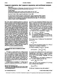
FIG. 1. Contours of ℜy1 and ℑy1 shown on the X plane for Van der Pol’s equation.

By integrating numerous trajectories outward from the vicinity of the equlibrium, and keeping track of the yi coordinate values crossed, Fig. 1 is produced. It shows the y frame coordinate grid with a contour separation of 0.1, and since the two coordinates y1 and y2 are always complex conjugate for real valued x, we have shown contours of ℜy1 and ℑy1 . The limit cycle is shown on the outside for comparison. [Some breaks in the contours are numerical artefacts.] The origin of the y frame is at the equlibrium, and it can be seen that the coordinate frame is collapsing as the limit cycle is approached. This is, however, done maintaining a constant determinant for the E matrix. Apparently any coordinate frame tied to

(54)

which is found by differentiating (18). This may be integrated to track the y2 coordinate. The non–canonical case is somewhat more difficult, since the diagonal Ω˙ ii are not necessarily zero. Again assuming a second order system, the diagonal entries are given by (41). For a second order system, we write 7

the limit cycle will not match smoothly with the modal coordinate frame tied to the equlibrium point at the origin.

result, with a contour √ interval of 0.1. Near the equlibrium we have Ω˙ i = 0.5 ± i 3/2, the value from the constant coefficient system. The two local exponents remain complex conjugate across the X plane. The plot terminates on the limit cycle, since no trajectories from the equlibrium can cross this line.

3 2

3

ℑ y1

1 0

2

-1

1 x2

-2 -3

0 -1

-4 -4

-3

-2

-1

0 ℜ y1

1

2

3

4

-2 -3

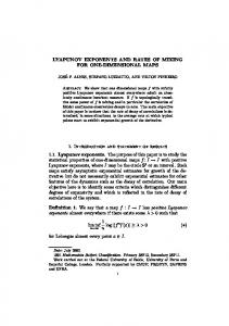
FIG. 2. Van der Pol trajectories in the ℜy1 , ℑy1 plane.

-4

Another interesting way to show the trajectories is to plot them in the y frame itself, Fig. 2. Since the plot again shows the real part ℜy1 versus the imaginary part ℑy1 , the trajectories should not really cross each other, even in the y frame. To the extent that they do, we have pushed the numerical calculation too far in an attempt to discover what the limit cycle maps to in the new coordinate frame. The problem occurs because the individual vectors of the E matrix grow at nearly the correct rate that the yi become constant as the limit cycle is approached.

x2

-1 -2 -3 1

2

1

2

3

4

(58)

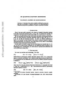
as a way to explore this problem. Figure 4 shows the y frame [with a contour interval of 0.2] for the pendulum with a damping factor of c = 0.25. The y frame is relatively flat near the equlibrium point, but becomes severely distorted as the separatrices are approached. As the damping factor is decreased towards zero, this twisting of the coordinate frame becomes more and more severe near the origin, and the zone of validity of the linearization about the equlibrium becomes smaller and smaller. Then, as c → 0, the twist of the coordinate frame tied to the equlibrium point becomes infinite. However, this is just what is observed numerically with (25) [but not (24)] as the damping vanishes. Apparently this is structural, since it occurs for any choice of local stability exponents that the author has investigated. So, it appears to be impossible to use the equlibrium point decomposition to define a global coordinate frame when the equlibrium is a center or a saddle.

0

0 x1

0 x1

x˙ 1 = x2 , x˙ 2 = −cx˙ − sin x = 0

1

-1

-1

The equlibrium point decomposition fails when stability exponents occur as positive / negative pairs, including centers, saddles, and in particular all Hamiltonian equlibrium points. We have used the damped pendulum

2

-2

-2

FIG. 4. Contours of ℜy1 and ℑy1 for the damped pendulum.

3

-3

-3

3

˙ on the X plane. FIG. 3. Contour plot of Ω



A similar technique can be used to examine the behav˙ i (X. Sampling traior of the local stability exponents Ω jectories eminating from the equlibrium point, we have kept track of where certain values of Ω˙ i are crossed, and then combined these into contours. Figure 3 shows the 8

∂gi c = Maxij − Ω˙ i δij , ∂yj

4 3

and the maximum violation of the symmetry condition for a coordinate frame ∂Eij ∂Eik (62) − d = Maxjk ∂yk ∂yj

2 1 x2

(61)

0 -1

as functions of time. Since these integrations extend from a point very close to the equlibrium well into the nonlinear regieme, and since solution of a boundary value problem is required to obtain the points necessary for the numerical partial derivatives, the author feels that some numerical error growth is inevitable.

-2 -3 -4 -3

-2

-1

0 x1

1

2

3

FIG. 5. Three y coordinate frames based on the periodic orbits of the undamped pendulum.

This does not mean that coordinate decompositions do not exist for the undamped pendulum. Figure 5 shows three y frames based on periodic orbits which are canonical, and between them cover the entire phase plane. The y1 directions are along the periodic orbits. The construction was made with the maximum value of y1 as 2π, since clearly y1 topologically looks like an angle near the stable equlibrium. The stable equlibrium is obviously a singular point for this coordinate frame, and furthermore the saddle point at x = ±π is also a singular point for all three y coordinate frames. We have sought numerical confirmation that using the methods of section IV actually produces a decoupling coordinate transformation. In particular, we have attempted to calculate the matrix ∂gi /∂yj , the gradient vector ∂ |E| /∂yi and ∂Eij /∂yk . The first should be di˙ i , the second agonal, with non–zero entries ∂gi /∂yi = Ω should be identically zero, while the last quantity should be symmetric in j and k if Y is a true coordinate frame. To calculate a numerical partial derivative, we have used Lagrangian five point numerical derivatives. Each numerical partial requires integrating a sheaf of five trajectories from the vicinity of the equlibrium to straddle the current point. Since it is common to use equal spacing in these points, we have solved a boundary value problem to find initial x values that produce equal spacing in the yi coordinate. As we have chosen to make these displacements real, this means that it is necessary to integrate the physical system off of the real x axis. Explicitly, we have plotted the quantities a = ||E(t)| − |E(t0 )|| ,

10

-2

10

-4

10

-6

10

-8

error

b c

10

-10

10

-12

10

-14

10

-16

d

a

0

5

10

15

20

25

time

FIG. 6. Numerical checks of the decoupling coordinate frame for the damped pendulum.

Figure 6 shows the result of one such calculation for the damped pendulum with c = 0.25, a starting position within 0.001 radian of the origin, and whose ending position is well over 4 radians. After some initial error growth, all of these tests indicate that the time propagation method is indeed producing a true coordinate frame Y which separates the equations of motion. Similar results are shown in Fig. 7 for the Van der Pol system. Again the starting point is within 0.0001 units of the equlibrium, and the final point is quite close to the limit cycle. In this case error growth in the calculation of these four quantities is more pronounced than in the case of the pendulum. But the results confirm that the yi do decouple the equations of motion, and that the integration is conserving the determinant |E|. Confirmation of the symmetry condition is the worst numerical verification, since this quantity is the difference of two numerical partial derivatives. There is good theoretical reason to believe that each of these conditions are met.

(59)

the error in propagating the determinant of E, the maximum deviation of its gradient from zero, ∂ |E| , b = Maxi (60) ∂yi

the maximum error in the local diagonalization of the equations of motion

9

d c ab

error

10

[1] H.D.I. Abarbanel, R. Brown, and M.B. Kennel, Int. J. Mod. Phys. B, 5, 1347 (1991). [2] D. K. Arrowsmith and C. M. Place, An Introduction to Dynamical Systems, Cambridge University Press, Cambridge, p 72 ff, (1990). [3] B. Eckhardt and E. Yao, Physica D, 65, 100, (1993). [4] J. M. Greene and J. S. Kim, Physica D, 24, 213, (1987). [5] H. Haken, Phys. Let. A, 94, 71 (1983). [6] E. N. Lorenz, Physica D, 13, 90, (1984). [7] L. Meirovitch, Methods of Analytical Dynamics, McGraw–Hill, New York, p 213 (1970). [8] W. J. Rugh, Linear System Theory, Prentice–Hall, New Jersey, (1993). [9] A.F. Vakakis, L.I. Manevitch, Y.V. Mikhlin, V.N. Pilipchuk, and A.A. Zevin, Normal Modes and Localization in Nonlinear Systems, Wiley, New York, (1996). [10] W. E. Wiesel, Phys. Rev. A, 46, 7480, (1992). [11] W. E. Wiesel, Phys. Rev. E, 48, 4752, (1993). [12] W.E. Wiesel and D. J. Pohlen, Celest. Mech. and Dynamical Astronomy, 58, 81, (1994).

0

10

-1

10

-2

10

-3

10

-4

10

-5

10

-6

10

-7

10

-8

10

-9

d c

a b

0

2

4

6

8 time

10

12

14

16

FIG. 7. Numerical checks of the decoupling coordinate frame for Van der Pol’s equation.

VII. DISCUSSION AND CONCLUSIONS VIII. APPENDIX A.

In this paper we have shown that the problem of local stability exponents which integrate along a trajectory to give global stability exponents is fully equivalent to the problem of dynamical separation of variables. The choice of constant determinant for the modal matrix E seems compelling for dissipative systems, and is the only choice permitted for Hamiltonian systems. The local stability exponents introduced by this choice are invariant to any linear change of variables. This invariance is less than the total invariance familiar from constant coefficient linear systems and time-periodic systems, but is still broader than the degree of invariance permitted by standard Lyapunov exponents. We have presented methods which lead to decoupling transformations in the vicinity of equlibrium points, periodic orbits, and along general trajectories eminating from equlibrium points. Such decoupling transformations may not exist in the vicinity of center and saddle point equlibria when the stability exponents of the equlibrium exist as positive/negative pairs. However, in this case it appears possible to base decoupling coordinate transformations on the surrounding periodic orbits. Much work remains to be done. We are currently exploring control applications, as well as continuing work on decoupling transformations near periodic orbits. Another area of interest is the relation of this method to the “geometrodynamics” approach, which attempts to decouple the trajectories of a dynamical system, and not necessarily the underlying equations of motion. Our method is based on decoupling the equations of motion, but seems to become a trajectory–based decoupling for Hamiltonian systems.

The form of the separation conditions near the equlibrium suffer from the fact that the “columns” of the partial derivatives of E are coupled. We have used equations (24) and (25) for numerical checks, and have employed an alternate form for the solution that is more efficient numerically. Instead of beginning with the separation conditions, begin with the modal matrix equation of motion (13), written as   ∂Eji −1 Ajα − Ω˙ i δjα Eαi = E fα . (63) ∂yβ βα Evaluation at the equlibrium point immediately yields the eigenvalue / eigenvector problem for the first order terms. Then, taking a partial derivative, evaluating at the equlibrium, and simplifying there results Ajα

∂Eαi ˙ i ∂Eji − Ω˙ k ∂Eji −Ω ∂yk ∂yk ∂yk ˙i ∂Ω ∂Ajα − δki Eji = − Eγk Eαi . ∂yi ∂xγ

(64)

The advantage of this form is that each “column” (e.g. index i) is decoupled from all the others, reducing the order of the linear system by a factor of N , the order of ˙ i /∂yi the dynamical system. Treating the quantities ∂ Ω as known, we must solve N systems of N 2 linear equations, not one system of order N 3 . Continuing to the third order gives Ajα − 10

 ∂2E  ∂ 2 Eαi ji − Ω˙ i + Ω˙ k + Ω˙ l ∂yk ∂yl ∂yk ∂yl

∂ 2 Ω˙ i ∂ 2 Ajα E δ δ = − Eǫl Eδk Eαi ji ki li ∂yi2 ∂xδ ∂xǫ

  ∂Ajα ∂Eαi ∂Eδk ∂Eαi Eδl + Eαi + Eδk ∂xδ ∂yk ∂yl ∂yl ˙ ˙ ∂ Ωi ∂Eji ∂ Ωi ∂Eji + δil + δki (65) ∂yi ∂yk ∂yi ∂yl ∂Eji −1 ∂Eδl ˙ ∂Eji −1 ∂Eδk ˙ − Eτ δ Ωl − E Ωk ∂yτ ∂yk ∂yτ τ δ ∂yl ∂Eγk ∂Eji −1 ∂Aαγ ∂Eji −1 E Aαγ + E Eγk Eτ l . + ∂yτ τ α ∂yl ∂yβ βα ∂xτ −

This form also has the “column” separation property, since all of the second partials of E with second index i can be solved for at once. Table I. Van der Pol Equlibrium Decomposition Order 1 ˙1 Ω 0.50000000000000 + 0.86602540378444i e11 0.70710678118655 + 0.i e21 0.35355339059327 + 0.61237243569579i ˙2 Ω 0.50000000000000 − 0.86602540378444i e12 0.70710678118655 + 0.i e22 0.35355339059327 − 0.61237243569579i Order 2 ˙ 11 Ω 0. + 0.i e111 0. + 0.i e112 0. + 0.i e211 0. + 0.i e212 0. + 0.i ˙ 22 Ω 0. + 0.i e121 0. + 0.i e122 0. + 0.i e221 0. + 0.i e222 0. + 0.i Order 3 ˙ 111 Ω −1.00000000000000 + 0.i e1111 0.0951874513135 − 0.0235527859883i e1112 −0.53033008588991 + 0.30618621784790i e1121 −0.53033008588991 + 0.30618621784790i e1122 −0.53033008588991 − 0.30618621784790i e2111 −0.50313367122889 + 0.21197507389470i e2112 −1.0606601717798 + 0.i e2121 −1.0606601717798 + 0.i e2122 −1.0606601717798 + 0.i ˙ 222 Ω −1.00000000000000 + 0.i e1211 −0.53033008588991 + 0.30618621784790i e1212 −0.53033008588991 − 0.30618621784790i e1221 −0.53033008588991 − 0.30618621784790i e1222 0.0951874513135 + 0.0235527859883i e2211 −1.0606601717798 + 0.i e2212 −1.0606601717798 + 0.i e2221 −1.0606601717798 + 0.i e2222 −0.50313367122889 − 0.21197507389470i

11