Stabilization of linear impulsive systems under dwell-time ... - HAL-Inria

Stabilization of linear impulsive systems under dwell-time constraints: Interval observer-based framework Kwassi Holali Degue, Denis Efimov, Jean-Pierre Richard

To cite this version: Kwassi Holali Degue, Denis Efimov, Jean-Pierre Richard. Stabilization of linear impulsive systems under dwell-time constraints: Interval observer-based framework. European Journal of Control, Lavoisier, 2018, .

HAL Id: hal-01761831 https://hal.inria.fr/hal-01761831 Submitted on 9 Apr 2018

HAL is a multi-disciplinary open access archive for the deposit and dissemination of scientific research documents, whether they are published or not. The documents may come from teaching and research institutions in France or abroad, or from public or private research centers.

L’archive ouverte pluridisciplinaire HAL, est destinée au dépôt et à la diffusion de documents scientifiques de niveau recherche, publiés ou non, émanant des établissements d’enseignement et de recherche français ou étrangers, des laboratoires publics ou privés.

1

Stabilization of Linear Impulsive Systems under Dwell-Time Constraints: Interval Observer-Based Framework Kwassi H. Degue, Denis Efimov, Jean-Pierre Richard

Abstract The problem of interval observer design is studied for a class of linear impulsive systems. Ranged and minimum dwell-time constraints are considered under detectability assumption. The first contribution of this paper lies in designing interval observers for linear impulsive systems under ranged and minimum dwelltime constraints, and investigating positivity of the estimation error dynamics in addition to stability. Several observers are designed oriented on different conditions of positivity and stability for estimation error dynamics. The boundedness of the estimation error (input-to-state stability property) and the observer stability conditions are stated as infinite-dimensional linear programming problems. Next, an output stabilizing feedback design problem is discussed, where the stability is checked using linear matrix inequalities (LMIs). Efficiency of the proposed approach is demonstrated by computer simulations for a commercial electric vehicle equipped with a low power range extender fuel cell, a bouncing ball, an academic linear impulsive system and for Fault Detection and Isolation (FDI) and Fault-Tolerant Control (FTC) of a power split device with clutch for heavy-duty military vehicles.

I. I NTRODUCTION There are many approaches dealing with the design techniques for state observers [1], [43], [27]. Frequently, these methods are based on (partial) linearity of the observed system, since analysis and design of stability and performance for linear systems are more developed. When it comes to take into account the presence of a disturbance or uncertain parameters, the synthesis of a conventional estimator (whose estimates are converging to the true values of the state) may be complicated [16], [1], [10], [11]. In such a case the problem of pointwise estimation can be substituted by the interval one, then using input-output measurements an observer has to estimate the set of admissible values (interval) for the state at each instant of time [30]. An advantage of interval observer is that it allows many types of uncertainties to be taken into account in the system. The interval observer design techniques have been developed for many types of models: continuous-time [38], [48], [9], discrete-time [16], [39], [21], [40], time-delay [41], [17], [18] and algebraic-differential [19] ones. K.H. Degue, D. Efimov and J.-P. Richard are with Inria, Non-A team, Parc Scientifique de la Haute Borne, 40 av. Halley, 59650 Villeneuve d’Ascq, France and CRIStAL (UMR-CNRS 9189), Ecole Centrale de Lille, BP 48, Cité Scientifique, 59651 Villeneuved’Ascq, France. K.H. Degue is with the Department of Electrical Engineering, Polytechnique Montreal and GERAD, Montreal, QC H3T-1J4, Canada. D. Efimov is with Department of Control Systems and Informatics, Saint Petersburg State University of Information Technologies Mechanics and Optics (ITMO), 49 Kronverkskiy av., 197101 Saint Petersburg, Russia. This work was supported in part by the Government of Russian Federation (Grant 074-U01); the Ministry of Education and Science of Russian Federation (Project 14.Z50.31.0031) and by the Fonds de recherche du Québec - Nature et technologies (FRQNT) international internships fellowship (Energy/Digital/Aerospace).

2

Continuing this line, the problem of design of interval observers for a class of linear hybrid systems [2], [29] is studied in this paper. Impulsive systems are an important class of hybrid systems that includes both continuous and discrete event dynamics. The continuous dynamics are generally represented by differential equations and the discrete ones by switching laws, which govern discontinuous jumps of continuous states [29], [26]. The instants of these jumps can be time-dependent or state-dependent [2], [29]. Some kinds of systems, like switched, sampled-time or impulsive ones for instance, can be presented in the hybrid framework. In the case of impulsive systems, dwell-times can be defined as the times between two consecutive impulses [3]. Unlike the stability problem for linear impulsive systems has been widely studied in previous works [34], [3], [44], [46], [32], little attention has been devoted to the observer design for this class of hybrid systems [42], [52]. In general, it is very difficult to assess the residual estimation error [37]. In opposition to this, interval observers provide bounds of this residual error at any time. The main peculiarity of interval observation is that it is necessary to ensure positivity of the estimation error dynamics in addition to their stability. Since two types of dynamics (continuous and discrete) are present in the hybrid systems, then the conditions of positivity for these two cases (see [20] for examples) have to be combined, which leads to variety of the applicability conditions and design structures proposed in this work. Only linear systems, where impulse instants can be inferred from the measured output or by using a sensor that detects mode transitions, are considered. Apart from the estimation problem complexity, output stabilization of impulsive systems is an important problem treated in the literature [24], [3], [7], [33]. The existing solutions in the literature are based on the assumption that the designed observers converge to the true values of the state. If only interval estimation is achievable, then the conventional approaches [49], [5], [54] cannot be applied, but interval observers demonstrated their efficiency for stabilizing control design in different classes of systems [23], [22], and in this work the approach is extended to impulsive systems. This paper sets out to make a contribution at two levels. Firstly, the design of interval observers for a class of hybrid systems (linear impulsive systems) is presented (a preliminary version of this part was given in [12]). Since impulsive systems are composed by continuous-time and discrete-time dynamics, and their interactions are governed by dwell time (the time between impulses), then the analysis of these systems is always based on some assumptions imposed on two parts independently, and dwell-time restrictions. For the design of interval observers, it is necessary to ensure positivity and stability of the estimation error dynamics, which has a hybrid nature in the considered case. Stability conditions for hybrid systems have been already developed. In the present paper the results of Theorems 1 and 2 given in Section II are used for ranged and minimal dwell time, respectively. We propose also an extension of the results from [3] on input-to-state stability analysis for linear impulsive systems. Positivity of hybrid dynamics has not been studied and analyzed in details in [3]. The synthesized observers take into account four sources of uncertainty: initial conditions for x(0), instant values of uncertain time-varying inputs in the continuous and discrete dynamics, and instant values of the measurement noise. It is assumed that all these uncertain factors belong to known intervals. Since in many applications the continuous or discrete dynamics of a linear impulsive system may not be observable, the proposed strategies just require the system to be detectable. The conditions of stability for the estimation error dynamics are formulated as matrix inequalities, which are nonlinear in the parameter θk := tk+1 − tk , that represents the dwell-time. For θk ∈ [Tmin , Tmax ] these matrix inequalities are infinite-dimensional feasibility problems: methods to solve them efficiently are also discussed in this work. Secondly, using the interval observers, a stabilizing control design based on

3

interval observers as in [23], [22] is presented. Since the interval estimates satisfy x(t) ≤ x(t) ≤ x(t) for all t ≥ 0, then the stabilization of the bounds x(t) and x¯(t) ensures the same property for the state x(t) of the considered linear impulsive system. To the best of our knowledge, interval observers approach has never been proposed for the stabilization of this class of hybrid systems. The outline of the paper is as follows. Some basic facts from the theories of interval estimation and hybrid systems are given in Section II, which contains also well-known conditions of positivity for continuous-time and discrete-time cases separately. Next, in Section III, we investigate conditions of hybrid systems robust stability under ranged dwell-time, which are applied in Sections IV and VI to design respectively interval observers and controller. Section IV presents three ways that are exploited to design interval observers having positive estimation error dynamics, starting from a simple combination in Theorem 3, then with a non-trivial uniting of different transformation of coordinates obtained for discrete-time and continuous-time parts in Theorem 4, and finally another generic scheme is presented in Theorem 5. Asymptotically exact computational approaches are proposed to solve infinite-dimensional feasibility observer stability conditions in Section V. A control design approach based on interval estimates for impulsive systems is studied in Section VI. In Section VII these results are applied to some examples of linear impulsive systems. The first example is a commercial electric vehicle equipped with a low power range extender fuel cell, the second one is a bouncing ball and the third example is an academic linear impulsive system. These three examples are devoted to estimation problem. The last one is a control problem of a power split device with clutch for heavy-duty military vehicles. Notation: In this work, the real and integer numbers are denoted by R and Z respectively, R≥0 = {τ ∈ R : τ ≥ 0} and Z≥0 = Z ∩ R≥0 , |x| is stated for the Euclidean norm of a vector x ∈ Rn . We denote respectively the cones of positive and nonnegative vectors of dimension n respectively by Rn>0 and Rn≥0 . For a bounded input u : R≥0 → R the symbol ||u||[t0 ,t1 ] denotes its L∞ norm: ||u||[t0 ,t1 ] = sup |u(t)|, t∈[t0 ,t1 ]

When t1 = +∞, we simply write ||u||. We denote by L∞ the set of all inputs u with the property ||u|| < ∞. The sequence of integers 1, ..., n is denoted by 1, n. En×m denotes the matrix with all entries equal 1 (with dimensions n × m). The vector of the eigenvalues of a matrix A ∈ Rn×n is denoted by λ(A). The relation P  0 (P  0) for a symmetric matrix P ∈ Rn×n means that it is n . The set of diagonal positive (nonnegative) definite, the set of such n × n matrices is denoted by S0 n matrices of dimension n is denoted by D and the subset of those being positive definite is denoted by Dn0 . II. P ROBLEM STATEMENT AND PRELIMINARIES Consider a hybrid (impulsive) linear system .

x(t) = Ax(t) + Bu(t) + f (t) ∀t ∈ [ti , ti+1 ), i ∈ Z≥0 , x(ti+1 ) = Gx(t− ∀i ≥ 1, i+1 ) + Du(ti+1 ) + g(ti+1 ) y(t) = Cx(t) + v(t),

(1)

m where x(t) ∈ Rn is the state vector and x(t− i+1 ) is the left-sided limit of x(t) for t → ti+1 ; u(t) ∈ R n×n n×m n is the control; A, G ∈ R ; B, D ∈ R ; f : R≥0 → R , f ∈ L∞ is the input for t ∈ [ti , ti+1 ); n 1 g : R≥0 → R , g ∈ C ∩ L∞ is the input at time instants ti+1 for i ≥ 1; y(t) ∈ Rp is the output signal

4

available for measurements; v ∈ L∞ is the measurement noise; C ∈ Rp×n . The sequence of impulse events ti with i ∈ Z≥0 is assumed to be positively incremental, i.e. θi = ti+1 − ti > 0 and t0 = 0. The matrices A, B, C, D, G are assumed to be known. Initial conditions for x(0), instant values of uncertain time-varying inputs in the continuous f and discrete g dynamics, and instant values of the measurement noise v are uncertain and included in known intervals. It is required to estimate a corresponding interval of admissible values for the state vector x(t) for all instants t ≥ 0, and next provide a solution of practical stabilization problem for the system (1) using the obtained interval estimates. The proposed control and estimation algorithms are based on the material presented below in this section. A. Interval analysis For two vectors x1 , x2 ∈ Rn or matrices A1 , A2 ∈ Rn×n , the relations x1 ≤ x2 and A1 ≤ A2 are understood elementwise. Given a matrix A ∈ Rm×n , define A+ = max{0, A}, A− = A+ − A (similarly for vectors) and denote the matrix of absolute values of all elements by |A| = A+ + A− . Lemma 1. [15] Let x ∈ Rn be a vector variable, x ≤ x ≤ x for some x, x ∈ Rn , and A ∈ Rm×n be a constant matrix, then A+ x − A− x ≤ Ax ≤ A+ x − A− x. (2) B. Nonnegative continuous-time linear systems A matrix A ∈ Rn×n is called Hurwitz if all its eigenvalues have negative real parts. It is called Metzler if all its elements outside the main diagonal are nonnegative, i.e. Ai,j ≥ 0 for 1 ≤ i 6= j ≤ n. Any solution of the linear system x(t) ˙ = Ax(t) + Bω(t), ω : R≥0 → Rq≥0 , y(t) = Cx(t) + Dω(t),

(3)

with x ∈ Rn , y ∈ Rp and a Metzler matrix A ∈ Rn×n , is elementwise nonnegative for all t ≥ 0 p×n provided that x(0) ≥ 0 and B ∈ Rn×q ≥0 [25], [50]. The output solution y(t) is nonnegative if C ∈ R≥0 p×q and D ∈ R≥0 . Such dynamical systems are called cooperative (monotone) or nonnegative if only initial conditions in Rn≥0 are considered [25], [50]. The stability of a Metzler matrix A ∈ Rn×n can be checked verifying a Linear Programming (LP) problem [25] AT λ < 0 for some λ ∈ Rn>0 . C. Nonnegative discrete-time linear systems A matrix A ∈ Rn×n is called Schur stable if all its eigenvalues have absolute value less than one, it is called nonnegative if all its elements are nonnegative (i.e. A ≥ 0). Any solution of the system xt+1 = Axt + Bωt , ω : Z≥0 → Rm ≥0 , t ∈ Z≥0

5

n×m with xt ∈ Rn and nonnegative matrices A ∈ Rn×n ≥0 and B ∈ R≥0 , is elementwise nonnegative for all t ∈ Z≥0 provided that x(0) ≥ 0 [35]. Such a system is called cooperative (monotone) or nonnegative [35]. n Lemma 2. [25] A matrix A ∈ Rn×n ≥0 is Schur stable iff there exists a diagonal matrix P ∈ S0 such T that A P A − P ≺ 0.

D. Stability of impulsive systems under ranged dwell-time and under minimum dwell-time constraints Consider an impulsive linear system with external inputs .

x(t) = Ax(t) + f (t) ∀t ∈ [ti , ti+1 ), i ∈ Z≥0 , x(ti+1 ) = Gx(t− i+1 ) + g(ti+1 ) ∀i ≥ 1,

(4)

where x(t) ∈ Rn is the state vector and x(t− i+1 ) is the left-sided limit of x(t) for t → ti+1 ; A, G ∈ n×n n R ; f : R≥0 → R , f ∈ L∞ is the input for t ∈ [ti , ti+1 ); g : R≥0 → Rn , g ∈ C 1 ∩ L∞ is the input at time instants ti+1 for all i ≥ 1. The sequence of impulse events ti with i ∈ Z≥0 is assumed to be positively incremental, i.e. θi = ti+1 − ti > 0 and t0 = 0. Theorem 1. [3], [4] Consider system (4) with ||f ||∞ = ||g||∞ = 0 and a ranged dwell-time θi ∈ [Tmin , Tmax ] for all i ∈ Z≥0 , where 0 < Tmin ≤ Tmax < +∞ are given constants. Then it n n such that for all and Q ∈ S0 is asymptotically stable provided that there exist matrices P ∈ S0 θ ∈ [Tmin , Tmax ] T GT eA θ P eAθ G − P = −Q. (5) Moreover, when the matrices A and G are respectively Metzler and nonnegative, the following statements are equivalent: (a) The impulsive system (1) is asymptotically stable under ranged dwell-time [Tmin , Tmax ]. (b) There exist a differentiable vector-valued function ψ : [0, Tmax ] 7→ Rn , ψ(0) ∈ Rn>0 , and a scalar  > 0 such that the inequalities .

ψ(τ )T A + ψ(τ )T ≤ 0 and T ψ(0)T G − ψ(θ)T + En×1 ≤0

hold for all τ ∈ [0, Tmax ] and θ ∈ [Tmin , Tmax ]. The proof of the first part of the above theorem is based on the fact that in this case V(x) = xT P x is a Lyapunov function for (4) at discrete instants of time ti . Let us consider now the minimum dwell-time case, θi ≥ Tmin for all i ∈ Z≥0 , for some given Tmin > 0. Theorem 2. [3], [4] Consider system (4) with ||f ||∞ = ||g||∞ = 0 and a dwell-time θi ∈ [Tmin , +∞) for all i ∈ Z≥0 , where Tmin is a given constant. Then it is asymptotically stable provided that there n exists a matrix P ∈ S0 such that AT P + P A ≺ 0, T AT Tmin

G e

Pe

ATmin

G − P ≺ 0.

(6)

6

Moreover when the matrices A and G are respectively Metzler and nonnegative, the following statements are equivalent: (a) The impulsive system (1) is asymptotically stable under minimum dwell-time Tmin . (b) There exists a differentiable vector-valued function ψ : [0, Tmin ] 7→ Rn , ψ(Tmin ) ∈ Rn>0 , and a scalar  > 0 such that the inequalities ψ(Tmin )T A < 0, .

ψ(τ )T A − ψ(τ )T ≤ 0, T ψ(Tmin )T G − ψ(0)T + En×1 ≤0 hold for all τ ∈ [0, Tmin ]. III. ROBUST STABILITY OF HYBRID SYSTEMS UNDER RANGED DWELL - TIME To the best of our knowledge, robust stability of linear impulsive systems with respect to the inputs under ranged dwell-time has never been proven before. Following [31], [8], robustness with respect to the inputs f and g can be proven (see the definition of the input-to-state stability (ISS) property given in those works). Lemma 3. Consider system (4) with a ranged dwell-time θi ∈ [Tmin , Tmax ] for all i ∈ Z≥0 , where n 0 < Tmin ≤ Tmax < +∞ are given constants. Then, provided that there exist matrices P ∈ S0 n and Q ∈ S0 such that for all θ ∈ [Tmin , Tmax ] the LMI (5) is satisfied, (4) is ISS and the following asymptotic gain is guaranteed lim |x(t)| ≤ [ρP,Q,W ||g||∞ + Tmax (1+

t→+∞

ρP,Q,W |G|%(A))||f ||∞ ]%(A), q λmax (W ) λmin (P )

ρP,Q,W = 1−

q

λmax (P )− 12 λmin (Q) λmin (P )

,

( eµ(A)Tmax where W = P + supθ∈[Tmin ,Tmax ] 2P GeAθ Qe GT P and %(A) = 1 T maxi=1,n λ( A+A ) being a logarithmic norm of the matrix A. 2 AT θ

Proof. From the system equations we can obtain for all i ∈ Z≥0 : Z t A(t−ti ) x(t) = e x(ti ) + eA(t−s) f (s)ds ∀t ∈ [ti , ti+1 ) ti

and x(ti+1 ) = GeATi x(ti ) + r(ti ) ∀i ≥ 1, where r(ti ) = G

R ti+1 ti

eA(ti+1 −s) f (s)ds + g(ti+1 ). Next, |eA(t−ti ) x(ti )| ≤ |eA(t−ti ) ||x(ti )| ≤ eµ(A)(t−ti ) |x(ti )|.

µ(A) > 0 for µ(A) = µ(A) ≤ 0

7

R ti+1 A(t−s) Let us denote φ = G ti e f (s)ds . One can write Z ti+1 φ ≤ |G| |eA(t−s) ||f (s)|ds t Z iti+1 ≤ |G| eµ(A)(ti+1 −s) |f (s)|ds (tRi t i+1 µ(A)Ti e |f (s)|ds µ(A) > 0 ti R ≤ |G| ti+1 |f (s)|ds µ(A) ≤ 0 t ( i Z eµ(A)Ti µ(A) > 0 ti+1 ≤ |G| |f (s)|ds 1 µ(A) ≤ 0 ti ≤ Ti |G|%(A)||f ||∞ . Therefore, |r(ti )| ≤ Ti |G|%(A)||f ||∞ + ||g||∞ and ||r||∞ ≤ Tmax |G|%(A)||f ||∞ + ||g||∞ . Consider a Lyapunov function V(x) = xT P x, where P ∈ Rn×n is given in LMI (5), then V(x(ti+1 )) − V(x(ti )) = xT (ti+1 )P x(ti+1 ) − xT (ti )P x(ti ) T

= xT (ti )[eA Ti GT P GeATi − P ]x(ti ) +2rT (ti )P GeATi x(ti ) + rT (ti )P r(ti ) ≤ −0.5xT (ti )Qx(ti ) + rT (ti )[P T

+2P GeATi QeA Ti GT P ]r(ti ) λmin (Q) V (x(ti )) + rT (ti )W r(ti ). ≤ − 2λmax (P ) From this expression we obtain 1 λmin (P )|x(ti+1 )|2 ≤ (λmax (P ) − λmin (Q))|x(ti )|2 + λmax (W )||r||2∞ 2 or equivalently for all i ≥ 1 s s λmax (P ) − 12 λmin (Q) λmax (W ) |x(ti+1 )| ≤ |x(ti )| + ||r||∞ . λmin (P ) λmin (P ) q λmax (P )− 12 λmin (Q) For i → +∞, since < 1, we derive that λmin (P ) |x(∞)| ≤ ρP,Q,W ||r||∞ . On any interval [ti , ti+1 ) the following estimate is satisfied |x(t)| ≤ eµ(A)(t−ti ) |x(ti )| + Tmax %(A)||f ||∞ ≤ [|x(ti )| + Tmax ||f ||∞ ]%(A)

8

for all t ∈ [ti , ti+1 ), then asymptotically the trajectories of (4) enter into the ball |x| ≤ [ρP,Q,W ||g||∞ + Tmax (1 + ρP,Q,W |G|%(A))||f ||∞ ]%(A) and the system is ISS. This result implies that (4) has bounded solutions for any bounded inputs f and g if the LMI (5) is valid. Consider system (4) with a dwell-time θi ∈ [Tmin , +∞) for all i ∈ Z≥0 , where Tmin is a given n constant. It can be inferred also that it is ISS provided that there exists a matrix P ∈ S0 such that the LMIs (6) are satisfied. IV. I NTERVAL OBSERVERS DESIGN The system (1) has four sources of uncertainty: initial conditions for x(0), instant values of f (t), g(t) and v(t). It is assumed that all these uncertain factors belong to known intervals. Assumption 1. The system (1) evolves under predetermined mode transitions, i.e. the impulse instants are known: θi = ti+1 − ti ∈ [Tmin , Tmax ] for all i ∈ Z≥0 , where 0 < Tmin ≤ Tmax < +∞ are given constants. Assumption 2. The state x(t) is bounded (i.e. x ∈ L∞ ) for x(0) ∈ [x(0), x¯(0)], and x(0), x¯(0) ∈ Rn are given constants. Assumption 3. Let i) two functions f , f : R≥0 → Rn , f , f ∈ L∞ be given such that f (t) ≤ f (t) ≤ f¯(t) ∀t ∈ R≥0 ; ii) two functions g, g : R≥0 → Rn , g, g ∈ C 1 ∩ L∞ be given such that g(t) ≤ g(t) ≤ g¯(t) ∀t ∈ R≥0 ; iii) the constant 0 ≤ V < +∞ be given such that ||v|| < V . Assumption 1 is common in the existing literature concerning stability analysis, observer and control design of hybrid systems [52], [31], [4], [3]. Assumption 2 is common in the existing literature concerning interval observer design. Assumptions 3.i and 3.ii state that the inputs of the hybrid system (1) are known up to some interval errors f¯(t) − f (t) and g¯(t) − g(t). Assumption 3.iii suggests an upper bound V for the noise v amplitude. A. Impulsive systems under ranged dwell-time constraints In this case we need additionally the following assumptions for the system (1): n n Assumption 4. There exist matrices L ∈ Rn×p , M ∈ Rn×p , P ∈ S0 and Q ∈ S0 such that i) the LMI T (G − M C)T e(A−LC) θ P e(A−LC)θ (G − M C) − P = −Q

holds for all θ ∈ [Tmin , Tmax ]; ii) the matrix (A − LC) is Metzler;

(7)

9

iii) the matrix (G − M C) is nonnegative. When Assumption 4.i holds, the quadratic form V(x) = xT P x is a discrete-time Lyapunov function for the LTI discrete-time system zi+1 = e(A−LC)θ (G − M C)zi for all θ ∈ [Tmin , Tmax ] and i ∈ Z≥0 by Theorem 1 (the matrix P can be selected diagonal since e(A−LC)θ (G − M C) is a nonnegative matrix for any θ ∈ [Tmin , Tmax ]). Assumptions 4.ii and 4.iii are essential for the approach but rather restrictive, they will be relaxed later. Under the introduced assumptions an interval observer equations for (1) take the form .

x(t) = (A − LC)x(t) + Ly(t) + Bu(t) + f (t) −LV ∀t ∈ [ti , ti+1 ), x(ti+1 ) = (G − M C)x(t− i+1 ) + M y(ti+1 ) +Du(ti+1 ) + g(ti+1 ) − M V,

(8)

.

x(t) = (A − LC)x(t) + Ly(t) + Bu(t) + f¯(t) +LV ∀t ∈ [ti , ti+1 ), x(ti+1 ) = (G − M C)x(t− i+1 ) + M y(ti+1 ) +Du(ti+1 ) + g(ti+1 ) + M V, ∀i ∈ Z≥0 , where x(t) ∈ Rn and x(t) ∈ Rn are the lower and the upper interval estimates for the state x(t), respectively, L = (L+ + L− )E p×1 and M = (M + + M − )E p×1 . Theorem 3. Let Assumptions 1, 2, 3 and 4 be satisfied. Then in (8) for all t ∈ R≥0 the discrepancies x(t) − x(t) and x(t) − x(t) are bounded and x(t) ≤ x(t) ≤ x¯(t)

(9)

provided that x(0) ≤ x(0) ≤ x¯(0). Proof. The equation (1) can be rewritten as follows .

x(t) = (A − LC)x(t) + Bu(t) + L[y(t) − v(t)] +f (t) ∀t ∈ [ti , ti+1 ), x(ti+1 ) = (G − M C)x(t− i+1 ) + Du(ti+1 ) + M [y(ti+1 ) − v(ti+1 )] +g(ti+1 ). Then the dynamics of the errors e(t) = x(t) − x(t), e(t) = x(t) − x(t) obey the equations for all i ∈ Z≥0 .

e(t) = (A − LC)e(t) + h1 (t) ∀t ∈ [ti , ti+1 ), e(ti+1 ) = (G − M C)e(t− i+1 ) + h2 (ti+1 ), .

e(t) = (A − LC)e(t) + h1 (t) ∀t ∈ [ti , ti+1 ), e(ti+1 ) = (G − M C)e(t− i+1 ) + h2 (ti+1 ),

(10)

10

where h1 (t) = [LV − Lv(t)] + [f (t) − f (t)], h2 (ti+1 ) = [M V − M v(ti+1 )] + [g(ti+1 ) − g(ti+1 )], h1 (t) = [LV + Lv(t)] + [f (t) − f (t)], h2 (ti+1 ) = [M V + M v(ti+1 )] + [g(ti+1 ) − g(ti+1 )]. According to Assumption 3, we have h1 , h1 , h2 , h2 ∈ L∞ ; h1 (t) ≥ 0, h1 (t) ≥ 0 ∀t ∈ [ti ; ti+1 ) and h2 (ti+1 ) ≥ 0, h2 (ti+1 ) ≥ 0 ∀i ≥ 1. When Assumption 4.i holds, the system (10) with ranged dwell-time θi ∈ [Tmin , Tmax ] is asymptotically stable for hk = hk = 0, k = 1, 2 and it has bounded state variables for bounded hk , hk (see Lemma 3). Therefore the variables e(t) and e(t) are bounded for the dwell-time θk ∈ [Tmin , Tmax ]. We continue having boundedness of the errors x¯(t) − x(t) and x(t) − x(t) as needed. From Assumptions 4.ii and 4.iii we conclude that e(t) ≥ 0 and e(t) ≥ 0 (h1 , h1 , h2 , h2 have the same property and e(0) ≥ 0 and e(0) ≥ 0 by conditions, then the result follows combining the theories presented in subsections II-B and II-C). That implies the required order relation x(t) ≤ x(t) ≤ x¯(t) is satisfied for all t ∈ R≥0 . Remark 1. The way the uncertainty (the interval widths ||f¯− f ||, ||¯ g − g||, |¯ x(0) − x(0)| and the value of V ) affects the accuracy of estimation of the current state is not discussed in this work. Indeed the interval width (the interval estimation accuracy) is proportional to the model uncertainty [6], and in order to optimize it, the stability conditions have to be reformulated in L2 /H∞ setting. However, to the best of our knowledge, there is no result of this kind for hybrid or impulsive systems with ranged or minimal dwell time, that is why only qualitative results are given in this paper. The imposed requirement, that the matrices A − LC and G − M C are Metzler and nonnegative respectively, is rather restrictive. In order to relax Assumptions 4.ii and 4.iii, let us suggest the following. n Assumption 5. There exist a Metzler matrix R, a matrix T ∈ Rn×n ≥0 and a matrix P ∈ S0 such that the LMI T T T eR θ P eRθ T − P ≺ 0 (11)

is satisfied for all θ ∈ [Tmin , Tmax ]. There exist a matrix L ∈ Rn×p and a matrix M ∈ Rn×p such that λ(A−LC) = λ(R), λ(G−M C) = λ(T ), the pairs (A − LC, e1 ), (R, e2 ), (G − M C, e3 ), (T, e4 ) are observable for some ej ∈ R1×n with j = 1, 4. When Assumption 5 holds, the quadratic form V(x) = xT P x is a Lyapunov function for linear discrete-time system zi+1 = eRθ T zi for all θ ∈ [Tmin , Tmax ] and i ∈ Z≥0 by Theorem 1. In addition, comparing with Assumptions 4.ii and 4.iii, in Assumption 5 it is proposed that the matrices A − LC and G − M C are similar to given Metzler and nonnegative matrices R and T , respectively [48], with different similarity transformation matrices S1 ∈ Rn×n and S2 ∈ Rn×n (i.e. S1−1 (A − LC)S1 = R and S2−1 (G − M C)S2 = T ). The key idea of the following design of an interval observer is how to combine these different transformations of coordinate S1 and S2 (denote S = (S1−1 S2 )−1 ), without introducing an auxiliary restriction.

11

Theorem 4. Let Assumptions 1, 2, 3 and 5 be satisfied. Then for all t ∈ R≥0 the discrepancies x(t) − x(t) and x¯(t) − x(t) are bounded and

x(t) ≤ x(t) ≤ x¯(t)

provided that x(0) ≤ x(0) ≤ x¯(0), where for all i ∈ Z≥0

x(t) = S1+ z1 (t) − S − 1 z1 (t), + x¯(t) = S1 z1 (t) − S − 1 z1 (t), z˙ 1 (t) = Rz1 (t) + F 1 y(t) − F1 V + (S1−1 )+ f (t) −(S1−1 )− f (t) ∀t ∈ [ti , ti+1 ), − − + − z2 (t− i+1 ) = S z1 (ti+1 ) − S z1 (ti+1 ), z2 (ti+1 ) = T z2 (t− i+1 ) + F 2 y(ti+1 ) − F2 V −1 + +(S2 ) g(ti+1 ) − (S2−1 )− g(ti+1 ), z1 (ti+1 ) = (S −1 )+ z2 (ti+1 ) − (S −1 )+ z2 (ti+1 ), . z1 (t)

(12)

(S1−1 )+ f (t)

= Rz1 (t) + F 1 y(t) + F1 V + −(S1−1 )− f (t) ∀t ∈ [ti , ti+1 ),

− − + − z2 (t− i+1 ) = S z1 (ti+1 ) − S z1 (ti+1 ),

z2 (ti+1 ) = T z2 (t− i+1 ) + F 2 y(ti+1 ) + F2 V −1 + +(S2 ) g(ti+1 ) − (S2−1 )− g(ti+1 ), z1 (ti+1 ) z1 (0) z1 (0) z2 (0) z1 (0)

= = = = =

(S −1 )+ z2 (ti+1 ) − (S −1 )+ z2 (ti+1 ), (S1−1 )+ x(0) − (S1−1 )− x(0), (S1−1 )+ x(0) − (S1−1 )− x(0), (S2−1 )+ x(0) − (S2−1 )− x(0), (S2−1 )+ x(0) − (S2−1 )− x(0),

−1 where F1 = S −1 1 L, F1 = |F1 |E p×1 , F2 = S 2 M and F2 = |F2 |E p×1 .

Remark 2. The proposed observer (12) contains interval observers for two sets of new coordinates z1 = S1−1 x and z2 = S2−1 x for continuous-time and discrete-time dynamics, respectively, with the corresponding transitions between them in the instants ti . Such an augmentation of the observer dimension allows us to avoid a restrictive assumption that there exists a common transformation of coordinates making the continuous-time and discrete-time parts positive simultaneously.

12

−1 −1 Proof. Consider the system (1) in the new coordinates z1 = S −1 z2 1 x, z2 = S 2 x, z1 = S .

z 1 (t) = Rz1 (t) + F 1 [y(t) − v(t)] +S1−1 f (t) + S1−1 Bu(t) ∀t ∈ [ti , ti+1 ), z2 (ti+1 ) = T z2 (t− i+1 ) + F 2 [y(ti+1 ) − v(ti+1 )] −1 +S2 g(ti+1 ) + +S2−1 Du(ti+1 ), y(t) = CS1 z 1 (t) + v(t) ∀t ∈ [ti , ti+1 ), y(ti+1 ) = CS2 z 2 (ti+1 ) + v(ti+1 ), z2 (ti+1 ) = (S + − S − )z1 (ti+1 ). The dynamics of the errors e1 (t) = z 1 (t) − z1 (t), e1 (t) = z1 (t) − z 1 (t), e2 (t) = z 2 (t) − z2 (t), e2 (t) = z2 (t) − z 2 (t) obey the equations for all i ∈ Z≥0 e˙ 1 (t) e2 (t− i+1 ) e2 (ti+1 ) e1 (ti+1 )

= = = =

Re1 (t) + h1 (t) ∀t ∈ [ti , ti+1 ), − − S + e1 (t− i+1 ) + S e1 (ti+1 ), T e2 (t− i+1 ) + h2 (ti+1 ), −1 + (S ) e2 (ti+1 ) + (S −1 )− e2 (ti+1 ),

(13)

.

e1 (t) = Re1 (t) + h1 (t) ∀t ∈ [ti , ti+1 ), − − + − e2 (t− i+1 ) = S e1 (ti+1 ) + S e1 (ti+1 ), e2 (ti+1 ) = T e2 (t− i+1 ) + h2 (ti+1 ), −1 + e1 (ti+1 ) = (S ) e2 (ti+1 ) + (S −1 )− e2 (ti+1 ), where h1 (t) = [F1 V − F 1 v(t)] + [(S −1 1 )f (t) −(S1−1 )+ f (t) + (S1−1 )− f (t)], h2 (ti+1 ) = [F2 V − F 2 v(ti+1 )] + [(S −1 2 )g(ti+1 ) −(S2−1 )+ g(ti+1 ) + (S2−1 )− g(ti+1 )], h1 (t) = [F1 V + F 1 v(t)] + [(S1−1 )+ f (t) −(S1−1 )− f (t) − (S −1 1 )f (t)], h2 (ti+1 ) = [F2 V + F 2 v(ti+1 )] + [(S2−1 )+ g(ti+1 ) −(S2−1 )− g(ti+1 ) − (S −1 2 )g(ti+1 )]. According to Assumption 3 we have h1 , h1 , h2 , h2 ∈ L∞ , h1 (t) ≥ 0, h1 (t) ≥ 0 ∀t ∈ [ti , ti+1 ) and h2 (ti+1 ) ≥ 0, h2 (ti+1 ) ≥ 0 ∀i ≥ 1. The matrix R is Metzler, the matrix T is nonnegative and these two matrices verify the LMI (11) when Assumption 5 is satisfied. Therefore, the system (13) with ranged dwell-time θi ∈ [Tmin , Tmax ] is asymptotically stable for hk = hk = 0, k = 1, 2 and it has bounded state variables for bounded hk , hk (see Lemma 3), then the variables e1 (t), e1 (t), e2 (t) and e2 (t) are bounded. Thus, the boundedness of z¯j (t) − zj (t), zj (t) − z j (t) for j = 1, 2, and next x¯(t) − x(t), x(t) − x(t), has been obtained. From the structure of the interval observer (12) and Assumption 5, since the matrix R is Metzler and the matrix T is nonnegative, we conclude that e1 (t) ≥ 0, e1 (t) ≥ 0,

13

e2 (t) ≥ 0 and e2 (t) ≥ 0 (h1 , h1 , h2 , h2 have the same property, e1 (0) ≥ 0, e1 (0) ≥ 0, e2 (0) ≥ 0 and e2 (0) ≥ 0 by construction, and the result follows combining the theories presented in subsections II-B and II-C). Thus, from the definitions of errors we conclude that for all i ∈ Z≥0 z1 (t) ≤ z 1 (t) ≤ z1 (t) ∀t ∈ [ti , ti+1 ), z2 (ti+1 ) ≤ z 2 (ti+1 ) ≤ z2 (ti+1 ) ∀i ≥ 1, which imply the relations of Theorem 4. There is another possibility for an interval observer construction avoiding the restrictions of Assumption 4, but with more conservative stability conditions. To this end, consider the following assumption. n Assumption 6. There exist a matrix L ∈ Rn×p , a matrix M ∈ Rn×p and a matrix P ∈ S0 such that the LMI T (14) J T eU θ P eU θ J − P ≺ 0     D0 D1 (G − M C)p (G − M C)n is satisfied for all θ ∈ [Tmin , Tmax ] and U = , J = for D1 D0 (G − M C)p (G − M C)n n×n A − LC = D0 − D1 where D0 is Metzler and D1 , (G − M C)p , (G − M C)n ∈ R≥0 .

Comparing with Assumption 5, here by construction the matrices U and J are Metzler and nonnegative respectively, i.e. these matrices can always be constructed satisfying these properties for any A − LC and G − M C (a possible but not unique choice is (G − M C)p = (G − M C)+ and (G − M C)n = (G − M C)− , for example), then there is no need in transformations of coordinates S1 and S2 . However, the main restriction is on the stability of such U and J, and the conditions of stability are formulated by LMI (14) following Theorem 1. The following result can be proven. Theorem 5. Let Assumptions 1, 2, 3 and 6 be satisfied. Then for all t ∈ R≥0 the discrepancies x(t) − x(t) and x¯(t) − x(t) are bounded and x(t) ≤ x(t) ≤ x¯(t) provided that x(0) ≤ x(0) ≤ x¯(0), where for all i ∈ Z≥0 : .

x(t) = D0 x(t) − D1 x(t) + Ly(t) + f (t) +Bu(t) − LV ∀t ∈ [ti , ti+1 ), − x(ti+1 ) = (G − M C)p x(t− i+1 ) − (G − M C)n x(ti+1 ) +Du(ti+1 ) + M y(ti+1 ) + g(ti+1 ) − M V, .

x(t) = D0 x(t) − D1 x(t) + Ly(t) + f (t) +Bu(t) + LV ∀t ∈ [ti , ti+1 ), − x(ti+1 ) = (G − M C)p x(t− i+1 ) − (G − M C)n x(ti+1 ) +Du(ti+1 ) + M y(ti+1 ) + g(ti+1 ) + M V, where L = |L|Ep×1 and M = |M |Ep×1 .

(15)

14

Proof. The equation (1) can be rewritten as follows for all i ∈ Z≥0 .

x(t) = (A − LC)x(t) + L[y(t) − v(t)] +Bu(t) + f (t) ∀t ∈ [ti , ti+1 ), x(ti+1 ) = (G − M C)x(t− i+1 ) + Du(ti+1 ) +M [y(ti+1 ) − v(ti+1 )] + g(ti+1 ). Then the dynamics of the errors e(t) = x(t) − x(t), e(t) = x(t) − x(t) obey the equations .

e(t) = D0 e(t) + D1 e(t) + h1 (t) ∀t ∈ [ti , ti+1 ), e(ti+1 ) = (G − M C)p e(t− i+1 ) +(G − M C)n e(t− i+1 ) + h2 (ti+1 ),

(16)

.

e(t) = D0 e(t) + D1 e(t) + h1 (t) ∀t ∈ [ti , ti+1 ), e(ti+1 ) = (G − M C)p e(t− i+1 ) +(G − M C)n e(t− i+1 ) + h2 (ti+1 ), where h1 (t) = [LV − Lv(t)] + [f (t) − f (t)], h2 (ti+1 ) = [M V − M v(ti+1 )] + [g(ti+1 ) − g(ti+1 )], h1 (t) = [LV + Lv(t)] + [f (t) − f (t)], h2 (ti+1 ) = [M V + M v(ti+1 )] + [g(ti+1 ) − g(ti+1 )]. According to Assumption 3 we have h1 , h1 , h2 , h2 ∈ L∞ , h1 (t) ≥ 0, h1 (t) ≥ 0 ∀t ∈ [ti , ti+1 ) and h2 (ti+1 ) ≥ 0, h2 (ti+1 ) ≥ 0 ∀i ≥ 1. If Assumption 6 is satisfied, then system (16) with ranged dwelltime θi ∈ [Tmin , Tmax ] is asymptotically stable for hk = hk = 0, k = 1, 2 and it has bounded state variables for bounded hk , hk (from Lemma 3). Therefore the variables e(t) and e(t) are bounded, and the discrepancies x(t) − x(t) and x¯(t) − x(t) inherit the same property. From the interval observer (15) structure and Assumption 6, since the matrix U is Metzler and the matrix J is nonnegative n×n (D0 is Metzler and D1 , (G − M C)p , (G − M C)n ∈ R≥0 ), we obtain that e(t) ≥ 0 and e(t) ≥ 0 (h1 , h1 , h2 , h2 have the same property, e(0) ≥ 0 and e(0) ≥ 0 by construction, and the result follows combining the theories presented in subsections II-B and II-C). Consequently, the required order relation x(t) ≤ x(t) ≤ x¯(t) is satisfied for all t ∈ R≥0 . The results of Theorems 4 and 5 can be combined, i.e. only one transformation S1 or S2 can be used together with the decomposition from Assumption 6. B. Impulsive systems under minimum dwell-time constraints The case of linear impulsive systems under minimum dwell-time constraints is considered in this section. We add the following assumptions for the system (1): Assumption 7. Let Tmax = +∞.

15

n Assumption 8. There exist matrices L ∈ Rn×p , M ∈ Rn×p , P ∈ S0 such that the LMIs

(A − LC)T P + P (A − LC) ≺ 0 and TT

(G − M C)T e(A−LC)

min

P e(A−LC)Tmin (G − M C) − P ≺ 0

are satisfied. When Assumption 8 holds, the quadratic form V(x) = xT P x is a discrete-time Lyapunov function for the LTI discrete-time system zi+1 = e(A−LC)θ (G − M C)zi for all θ ∈ [Tmin , +∞) and i ∈ Z≥0 by Theorem 2. Corollary 1. Let Assumptions 1, 2, 3, 4.ii, 4.iii, 7 and 8 be satisfied. Then the observer proposed in Theorem 3 can be applied. In order to relax Assumptions 4.ii and 4.iii, let us suggest the following. n Assumption 9. There exist a Metzler matrix R, a matrix T ∈ Rn×n ≥0 and a matrix P ∈ S0 such that the LMIs

RT P + P R ≺ 0, T T eR

TT

min

P eRTmin T − P ≺ 0

are satisfied. There exist a matrix L ∈ Rn×p and a matrix M ∈ Rn×p such that λ(A−LC) = λ(R), λ(G−M C) = λ(T ), the pairs (A − LC, e1 ), (R, e2 ), (G − M C, e3 ), (T, e4 ) are observable for some ej ∈ R1×n with j = 1, 4. Corollary 2. Let Assumptions 1, 2, 3, 7 and 9 be satisfied. Then the observer proposed in Theorem 4 can be applied. Like in section IV-A, there is another possibility for an interval observer construction avoiding the restrictions of Assumptions 4.ii and 4.iii, but with more conservative stability conditions. To this end, consider the following assumption. n Assumption 10. There exist a matrix L ∈ Rn×p , a matrix M ∈ Rn×p and a matrix P ∈ S0 such that the LMIs

U T P + P U ≺ 0, J T eU

TT min

P eU Tmin J − P ≺ 0



   D0 D1 (G − M C)p (G − M C)n are satisfied and U = , J = for A − LC = D0 − D1 D1 D0 (G − M C)p (G − M C)n n×n where D0 is Metzler and D1 , (G − M C)p , (G − M C)n ∈ R≥0 . Corollary 3. Let Assumptions 1, 2, 3, 7 and 10 be satisfied. Then the observer proposed in Theorem 5 can be applied.

16

Choice of two positive reals a and b such that the LMIs are feasible when Tmin=a and infeasible when Tmin=b

A← a B← b Precision← p

Yes

LMIs feasible when Tmin=(A+B)/2?

B← B

No

A← A

A← (A+B)/2

B← (A+B)/2

Display A and B

No

|A − B| ≤ 10−p

Yes End

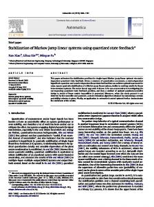
Figure 1. Flowchart of infinite dimensional feasibility LMI resolution procedure under minimum dwell-time constraints

V. C OMPUTATIONAL CONSIDERATIONS The conditions of Theorems 3, 4 and 5 are infinite-dimensional feasibility problems since, for example, 7, 11 and 14 are nonlinear in the parameter θ, and for θ ∈ [Tmin , Tmax ] these matrix inequalities consist of an infinite number of LMIs. Hence it is important to propose efficient methods to solve them. Let us discuss two approaches that can be used to solve these infinite-dimensional stability conditions.

A. First approach A first approach consists in selecting manually the gains L and M of the interval observer. Given these gains, a bisection-like approach is used to find the interval [Tmin , Tmax ] where the LMIs 7, 11 and 14 are feasible. Under minimum dwell-time constraints, the procedure used to solve infinitedimensional feasibility LMI problems is shown in Fig. 1, it finds an interval [A, B] for Tmin , then at the end Tmin = A. A similar process can be defined to solve infinite dimensional feasibility LMI problems under ranged dwell-time constraints.

17

B. Second approach Instead of using the θ-dependent matrix inequalities (5) and (6), the conditions dependent on ψ(t) from Theorems 1 and 2 can be applied for stability analysis. In this case, to ensure resolution of these conditions, the observer gains L and M have to be imposed to be time-varying, L(t) and M (t), respectively. In this subsection we assume that all corresponding positivity restrictions on L(t) and M (t) are satisfied (they are the same as for the constant gains) and put focus on stability issues. Assume that Tmin and Tmax (for the ranged dwell-time constraints) and Tmin (for the minimum dwell-time) are given. Taking into account these bounds, piecewise linear approximations of the function ψ can be introduced satisfying the conditions of Theorems 1 and 2 by semidefinite programming. However, as it is noted in [4], such an approximate method may show a poor convergence and high computational complexity. Then another approach consists in application of the so-called sum-of-squares (SOS) method [4], based on the result of [47]. An advantage of SOS tool is that verifying whether a polynomial is SOS can be formulated using semidefinite programs that can be solved by standards solvers using SOSTOOLS package [45]. For examples of application of this approach, the cases of Theorem 3 (ranged dwell-time) and Corollary 1 (minimum dwell-time) are considered in this section (other cases can be treated similarly). 1) Relaxation in Theorem 3 (ranged dwell-time): In this case, following [4], for the interval observer (8) the gain L is time-varying: ˆ − ti ) ∀t ∈ (ti , ti+1 ], i ∈ Z≥0 , L(t) = L(t ˆ : [0, Tmax ] 7−→ Rn×p is a matrix-valued function determined below: where L Proposition 1. Let X : [0, Tmax ] 7−→ Dn0 be a differentiable matrix-valued function, Uc : [0, Tmax ] 7−→ Rn×p be a matrix-valued function, Ud ∈ Rn×p be a matrix, and , α > 0 be scalars such that the inequalities X(τ )A − Uc (τ )C + αI ≥ 0, X(0)G − Ud C ≥ 0, i h. T En×1 X(τ ) + X(τ )A − Uc (τ )C ≤ 0

(17a) (17b)

and T En×1 [X(0)G − Ud C − X(θ) + I] ≤ 0

(18)

hold for all τ ∈ [0, Tmax ] and θ ∈ [Tmin , Tmax ]. If the gains of the interval observer (8) are computed as ˆ ) = X(τ )−1 Uc (τ ) and M = X(0)−1 Ud , L(τ then the conditions and the result of Theorem 3 are satisfied. Proof. The conditions in (17a) guarantee that the matrix A − L(τ )C is Metzler for all τ ∈ [0, Tmax ] and that the matrix G − M C is nonnegative. Using the change of variables ψ(τ ) = X(τ )En×1 , ˆ ) = X(τ )−1 Uc (τ ) and M = X(0)−1 Ud , one can remark that the conditions (17b) and (18) are L(τ equivalent to . ˆ )C) + ψ(τ )T ≤ 0, ∀τ ∈ [0, Tmax ] ψ(τ )T (A − L(τ T ψ(0)T (G − M C) − ψ(θ)T + En×1 ≤ 0, ∀θ ∈ [Tmin , Tmax ].

It can be inferred from Theorem 1 that this is equivalent to saying that the error dynamics (10) is asymptotically stable under ranged dwell-time [Tmin , Tmax ].

18

C. Relaxation in Corollary 1 (minimum dwell-time) Following [4], for the interval observer (8) we propose the following form for the gain L: ( ˆ − ti ) ∀t ∈ (ti , ti + τ ], i ∈ Z≥0 , L(t L(t) = ˆ L(Tmin ) ∀t ∈ (ti + Tmin , ti+1 ], i ∈ Z≥0 , ˆ : R≥0 7−→ Rn×p is a function determined below. where L Proposition 2. Let X : [0, Tmin ] 7−→ Dn0 be a differentiable matrix-valued function, Uc : [0, Tmin ] 7−→ Rn×p be a matrix-valued function, Ud ∈ Rn×p be a matrix, and , α > 0 be scalars such that the inequalities X(τ )A − Uc (τ )C + αI ≥ 0, X(Tmin )G − Ud C ≥ 0, i T En×1 X(Tmin )A − Uc (Tmin )C + αI ≤ 0, h . i T En×1 −X(τ ) + X(τ )A − Uc (τ )C ≤ 0 h

(19a)

.

(19b) (19c)

and T En×1 [X(Tmin )G − Ud C − X(0) + I] ≤ 0

(20)

hold for all τ ∈ [0, Tmin ]. Hence, the gains of the interval observer (8) can be computted as follows ˆ ) = X(τ )−1 Uc (τ ) and M = X(Tmin )−1 Ud . L(τ Proof. The conditions in (19a) guarantee that the matrix A − L(τ )C is Metzler for all τ ∈ [0, Tmin ] and that the matrix G − M C is nonnegative. Using the change of variables ψ(τ ) = X(τ )En×1 , ˆ ) = X(τ )−1 Uc (τ ) and M = X(Tmin )−1 Ud , one can remark that the conditions (19b) , (19c) and L(τ (20) are equivalent to ˆ )C) < 0, ψ(Tmin )T (A − L(τ .

ˆ )C) − ψ(τ )T ≤ 0, ψ(τ )T (A − L(τ T ψ(Tmin )T (G − M C) − ψ(0)T + En×1 ≤ 0. It can be inferred from Theorem 2 that this is equivalent to saying that the error dynamics (10) are asymptotically stable under minimum dwell-time Tmin . VI. C ONTROL DESIGN The idea of this work consists in solving the stabilization problem for the completely known system (8) instead of (1). Under conditions of Theorem 3, if both x(t) and x¯(t) converge to zero, then the state x(t) also has to converge to zero, and boundedness of x(t) follows by the same property of x(t) and x¯(t). In this case the signal y(t) is treated in the system (8) as a state dependent disturbance. Corollary 4. Let Assumptions 1, 3, 4.ii and 4.iii be satisfied, then |y(t)| ≤ |C|(|x(t)| + |¯ x(t)|),

∀t ∈ R≥0 .

Proof. Indeed, from (9) xk (t) ≤ xk (t) ≤ x¯k (t) ∀t ≥ 0 ∀k = 1, . . . , n

19

under conditions of Theorem 3, then |xk (t)| ≤ max{|xk (t)|, |¯ xk (t)|} and a straightforward computation shows 2

|x(t)|

= ≤

n X k=1 n X

2

|xk (t)| ≤

n X

xk (t)|2 } max{|xk (t)|2 , |¯

k=1

xk (t)|2 = |x(t)|2 + |¯ |xk (t)|2 + |¯ x(t)|2

k=1

or x(t)|. |x(t)| ≤ |x(t)| + |¯ Consequently, |y(t)| = |Cx(t)| ≤ |C||x(t)| ≤ |C|(|x(t)| + |¯ x(t)|) for all t ≥ 0. Hence, one has to stabilize the system (8) uniformly (or robustly) with respect to a Lipschitz nonlinearity y. The control is chosen as a conventional state linear feedback u(t) =Kx(t) + K x¯(t), ∀t ∈ [ti , ti+1 ), − u(ti+1 ) =Jx(t− i+1 ) + Jx(ti+1 ),

(21)

where K, K, J and J are four feedback gains to be designed. When substituting the control (21) into (8), it follows that .

x(t) = (A − LC + BK)x(t) + Ly(t) + BK x¯(t) + f (t) −LV ∀t ∈ [ti , ti+1 ), x(ti+1 ) = (G − M C + DJ)x(t− i+1 ) + M y(ti+1 ) +DJx(t− i+1 ) + g(ti+1 ) − M V,

(22)

.

x(t) = (A − LC + BK)x(t) + Ly(t) + BKx(t) + f¯(t) +LV ∀t ∈ [ti , ti+1 ), x(ti+1 ) = (G − M C + DJ)x(t− i+1 ) + M y(ti+1 ) − +DJx(ti+1 ) + g(ti+1 ) + M V, and it is necessary to analyse stability of this nonlinear system. Let us introduce ε(t) = [xT (t) x¯T (t)]T and the matrices   A − LC + BK BK R= , BK A − LC + BK   DJ G − M C + DJ S= , DJ G − M C + DJ     f (t) − LV g(ti+1 ) − M V δ(t) = ¯ , ς(ti+1 ) = , f (t) + LV g(ti+1 ) + M V

20

then one can rewrite the system (22) as   Ly(t) ε(t) ˙ =Rε(t) + δ(t) + Ly(t)   M y(ti+1 ) − ε(ti+1 ) =Sε(ti+1 ) + ς(ti+1 ) + . M y(ti+1 )

(23)

Theorem 6. Let Assumptions 1, 3, 4.ii and 4.iii hold, x(0) ≤ x(0) ≤ x¯(0) and there exist matrices 2n 2n K ∈ Rm×n , K ∈ Rm×n , J ∈ Rm×n , J ∈ Rm×n , P ∈ S0 and Q ∈ S0 such that the matrix inequality T

eR θ S T P eRθ − P + Q = 0 is satisfied for all θ ∈ [Tmin , Tmax ], and √ √ ρP,Q,W 2|M | + 2Tmax (1 + ρP,Q,W |S|%(R))|L|]%(R)|C| < 1,

(24)

(25)

T

where W = P + supθ∈[Tmin ,Tmax ] 2P SeRθ QeR θ S T P . Then the system (1), (8), (21) is ISS with respect to the inputs δ and ς. Proof. Since Assumptions 4.ii, 4.iii and 3 are satisfied, then all conditions of Theorem 3 are verified, and the interval inclusion (9) holds. By construction, (9) is true for any input u, and for the control (21) in particular. After substitution of (21) in (1) and (8), the dynamics of (8) can be presented in the form of (23), where according to Corollary 4 the variable y can be considered as a nonlinear function of the state of (23) |y| ≤ |C||ε|. If there exist matrices K, K, J, J, P and Q such that the matrix inequality (24) is satisfied, then according to Lemma 3 the system (23) is ISS with respect to the auxiliary inputs     Ly(t) M y(ti+1 ) f (t) = δ(t) + , g(ti+1 ) = ς(ti+1 ) + , Ly(t) M y(ti+1 ) which contain the state-dependent function y. From the asymptotic gain property established in Lemma 3, we know that asymptotically the trajectories enter in the ball |ε| ≤ [ρP,Q,W ||g||∞ + Tmax (1 + ρP,Q,W |S|%(R))||f ||∞ ]%(R) √ ≤ [ρP,Q,W (||ς||∞ + 2|M ||y|) + Tmax (1 + √ ρP,Q,W |S|%(R)) × (||δ||∞ + 2|L||y|)]%(R) = [ρP,Q,W ||ς||∞ + Tmax (1 + ρP,Q,W |S|%(R))||δ||∞ ] √ √ ×%(R) + [ρP,Q,W 2|M | + 2Tmax (1 + ρP,Q,W |S|%(R))|L|]%(R)|y| ≤ [ρP,Q,W ||ς||∞ + Tmax (1 + ρP,Q,W |S|%(R))||δ||∞ ] √ √ ×%(R) + [ρP,Q,W 2|M | + 2Tmax (1 + ρP,Q,W |S|%(R))|L|]%(R)|C||ε|.

21

Table I PARAMETERS USED IN THE A PPLICATION Param. Lf c RLf c iLf c uf c uch1 Ftrac Fres Mtot vveh f g α Cx ρ vwind A

Meaning inductance of the smoothing inductor resistance of the smoothing inductor smoothing inductor’s current fuel cell’s voltage one of the two chopper’s voltages traction force resistive forces equivalent total mass of the chassis vehicle’s velocity rolling resistance coefficient acceleration due to gravity slope rate air drag coefficient mass density of the considered fluid wind’s velocity frontal area

Therefore, by the standard small-gain arguments, if the condition (25) is satisfied, then the asymptotic gain property is validated |ε| ≤

[ρP,Q,W ||ς||∞ + Tmax (1 + ρP,Q,W |S|%(R))||δ||∞ ]%(R) √ √ , 2|M | + 2Tmax (1 + ρP,Q,W |S|%(R))|L|]%(R)|C|

1 − [ρP,Q,W

and the system (23) is ISS with respect to the inputs δ and ς. VII. A PPLICATIONS In this section, four examples are presented. The first example is a commercial electric vehicle equipped with a low power range extender fuel cell, the second one is a bouncing ball and the third example is an academic linear impulsive system. These three examples are devoted to estimation problem. The last one is a control problem of a power split device with clutch for heavy-duty military vehicles. A. Case of Theorem 3 A commercial electric vehicle equipped with a low power range extender fuel cell system is considered [13]. The regenerative braking is assumed sufficient to stop the vehicle (no mechanical braking) and the induction machine is replaced by a permanent magnet DC machine supplied by a chopper from the battery (see Fig. 2). With reference to the notation in Table I, the smoothing inductor of the fuel cell system can be represented by the following equation d Lf c iLf c = uf c − uch1 − RLf c iLf c . dt Using the Newton’s second law, we obtain Mtot

d vveh dt Fres

=

Ftrac − Fres

=

f Mtot g + 0.5ρCx A(vveh + vwind )2 + Mtot gα.

22

Figure 2. Fuel Cell range extension of the considered vehicle [13]

Horizontal surface is considered in this example, then α = 0. Let us consider an abstract failure mode scenario of the electric vehicle where uf c = uch1 and −1 0.5ρCx A = ζMtot vveh for all t 6= 10 + 20k with k ∈ N, where ζ is a given constant. Discrete dynamics appear for the system in this failure mode for t = 10 + 20k, k ∈ N. The force resisting the R c motion when the vehicle rolls on the surface is neglected (f = 0). The case where LLf = γ = 1.5 fc and ζ = 0.1 is considered. In this abstract scenario, let us neglect the traction force and the wind’s velocity. That is, Ftrac = 0 and vwind = 0. Additional uncertain time-varying inputs are injected to the continuous dynamics and to the discrete ones, then this failure mode can be represented by the following system with x(t) = [iLf c (t) vveh (t)]T .

x(t) = Ax(t) + b(t) ∀t 6= 10 + 20k, k ∈ N, x(t) = Gx(t− ) + d(t) ∀t = 10 + 20k, k ∈ N, y(t) = Cx(t) + v(t), where the matrices A, C and G are defined as follows       −γ 0 1.8 0 A= , C= 0 1 , G= , 0 −ζ 1.2 0.7 and x(t) ∈ R2 , y(t) ∈ R are the state and the output, respectively. The signals b(t), d(t) and v(t) are     β sin(2t) δ sin(t) + 0.3 b(t) = , d(t) = , β sin(2t) δ sin(t) + 0.3 v(t) = V sin(t), where β = 0.1, δ = 0.1 and V = 0.1 are known parameters. Thus,     −β β b(t) = , b(t) = , −β β     −δ + 0.3 δ + 0.3 d(t) = , d(t) = . −δ + 0.3 δ + 0.3 Assumption 3 is then satisfied. One can remark that in this case, the pair (A, C) is not observable, but doing the PBH (Popov–Belevitch–Hautus) test for the eigenvalues of the matrices A, it can be easily proved that the pair (A, C) is detectable. Assumption 4.ii is verified when we choose    T −1.5 0 L = 0 2.6 : the matrix A − LC = is Metzler. Assumption 4.iii is verified 0 −2.7

23

Figure 3. Results of the simulation for the case of Theorem 3

 1.8 0 is nonnegative but not Schur when one selects M = 0 0.4 : the matrix G − M C = 1.2 0.3 stable. By applying Matlab YALMIP toolbox [36] to solve the LMIs we found that Assumption 8 holds for all θ ∈ [0.3919, +∞). Then the system (10) with the minimum dwell-time Tmin = 0.3919 is ISS. Therefore all conditions of Corollary 1 are satisfied and the interval observer (8) solves the problem of interval state estimation. The results of simulation are shown in Fig. 3, where the solid lines represent the states xk , k = 1, 2 and the dash lines are used for the interval estimates xk and xk . 

T



B. Case of Theorem 4 Consider the case of vertical motion of a ball under gravity with a constant acceleration g. The dynamics are given by . . p(t) = v(t); v(t) = −g, where p(t) ∈ R≥0 is the position of the ball and v(t) ∈ R is its velocity, which is assumed to be downward. Upon hitting the ground at instant of time t0 ≥ 0 with p(t0 ) = 0, we instantly set v(t0 ) to -ρv(t0− ), where ρ ∈ [0, 1] is the coefficient of restitution. In general, this model can be presented in the form of system (1) = [p(t) v(t)]T , = Ax(t) + b(t) when x1 (t) 6= 0, = Gx(t− ) + d(t) when x1 (t) = 0, = Cx(t),       0 1 1 0 where A = ,C= 1 0 ,G= ; x(t) ∈ R2 , y(t) ∈ R are respectively the state 0 0 0 −ρ and the output; the signals b(t) and d(t) model some additional perturbing forces applied to the ball     β sin(t) δ sin(t) , d(t) = , b(t) = −g + β sin(t) δ sin(t) x(t) . x(t) x(t) y(t)

24

Figure 4.

Results of the simulation for the case of Theorem 4

where β = 0.5 and δ = 0.5 are known parameters. Thus,    −β β b(t) = , b(t) = , −g − β −g + β     −δ δ d(t) = , d(t) = −δ δ 

and Assumption 3 is then satisfied. Assume that ||x|| < +∞ (Assumption 7 is valid). Verifying the LMIs with Matlab YALMIP toolbox [36], we found that Assumption 9 holds for any minimum dwell-time Tmin > 0. Therefore, all conditions of Corollary 2 are satisfied. Finally, the matrices    −2 0 −0.7071 −0.4472 , S1 = , R= 0 −1 −0.7071 −0.8944     −0.8 0 0 0.9594 T = , S2 = 0 0.9 1 0.2822 

satisfy all conditions of Theorem 4 and the interval observer (12) solves the problem of interval state estimation for bouncing ball. The results of simulation are shown in Fig. 4, where the solid lines represent the states xk , k = 1, 2 and the dash lines are used for the interval estimates xk and xk . Remark 3. In the example of the bouncing ball considered in this work, the measurement noise is equal to zero. This means the times of the jumps in the state are well estimated as the output signal is supposed to be perfect (without noise). In the real case, there is always a measurement noise in the output signal: the jump times in the state are not known and need to be estimated. It may introduce a time-delay in the estimated jumping time and causes some additional error in the state estimation.

25

C. Case of Theorem 5 Let us denote by Λ the set of transition times of the clock signal in Fig. 5 when its changes from one to zero (rising times). Consider the following system .

x(t) = Ax(t) + b(t) ∀t ∈ R≥0 \ Λ, x(t) = Gx(t− ) + d(t) ∀t ∈ Λ, y(t) = Cx(t), where the matrices A, C and G are defined as follows       −2 0 2 0 A= , C= 1 0 , G= 0 −1 1 −0.2 and x(t) ∈ R2 , y(t) ∈ R are respectively the state and the output. The signals b(t) and d(t) are     β sin(2t) cos(t) 0.2 + δ sin(t) b(t) = , d(t) = β sin(2t) cos(t) 0.2 + δ sin(t) with known β = 0.1 and δ = 0.1. Thus, 

−β −β





β β



, b(t) = , b(t) =     −δ + 0.2 δ + 0.2 d(t) = , d(t) = . −δ + 0.2 δ + 0.2 Assumption 3 is then satisfied. One can remark that in this case, the pairs (A, C) and (G, C) are not observable. Doing the PBH test for the eigenvalues of the matrices A and G, it canbe easily proved   T −2 0 , we that the pairs (A, C) and (G, C) are detectable. For L = 0 4 and A − LC = −4 −1 choose     −1.5 0 0.5 0 , D1 = , D0 = 0 −1 4 0  T n×n then D0 is Metzler and D1 ∈  R≥0 . Note that the matrix A−LC is not Metzler. For M = −1 2.8 2 1 and G − M C = , we choose 1 −3     2.5 1 0.5 0 (G − M C)p = , (G − M C)n = . 1 0 0 3 n×n (G − M C)p ∈ Rn×n ≥0 and (G − M C)n ∈ R≥0 . Note that the matrix G − M C is negative and is not Schur stable. By applying Matlab YALMIP toolbox [36] to solve the LMIs we found that Assumption 10 holds for all Tk ∈ (2.7579, +∞). Therefore, all conditions of Corollary 3 are satisfied and the interval observer (15) solves the problem of interval state estimation. The results of simulation are shown in Fig. 5, where the solid lines represent the states xk , k = 1, 2 and the dash lines are used for the interval estimates xk and xk .

26

Figure 5. Results of the simulation for the case of Theorem 5

D. Case of output stabilizing feedback using control of Theorem 6 Let us apply now the stabilizing feedback control that has been designed in this paper to Fault Detection and Isolation (FDI) and Fault-Tolerant Control (FTC) of a complex uncertain system. Hybrid electric vehicles (HEVs) can be classified with respect to their energy flow used for propulsion as either series or parallel [51]. Combining these two systems one can obtain the so-called series-parallel HEVs, which have the advantages of these two basic architectures, but have a more complicated structure. The Power Split Device (PSD) that divides the power coming from various power sources into the drivetrain (see Fig. 2) plays a major role in the suitable energy management strategy of series-parallel HEVs [28]. A hybrid powertrain with a high availability for heavy-duty military vehicles is considered for our application. A series-parallel HEV architecture is considered along with the Ravigneaux geartrain as PSD [51]. The considered architecture is comprised of a PSD mounted with shafts connected to two electric machines (EM1 and EM2) through gearboxes, an Internal Combustion Engine (ICE) and transmission with clutch through a gearbox [51] (see Fig. 3). The role of a clutch is to connect the driving shaft to a driven shaft, so that the driven shaft may be started or stopped at will, without stopping the driving shaft. In conventional vehicles, the clutch allows for power to be transmitted from the ICE to the wheels in order to change the speed ratio using the gearbox [51]. The behavior of the clutch is nonlinear, and two different states are considered: the slipped (open) one and the locked (closed) one. During the locked position of the clutch, the system is considered as a single equivalent inertia: the disks are rigidly coupled with each other. With reference to the notation in Table II, the locked position of the clutch can be modeled by the

27

Figure 6. Series-Parallel HEV Configuration with PSD [51]

Figure 7. Considered System Layout [51]

following equations

JCL1

d ΩCL + fCL1 ΩCL = TCL2 − TP C , dt TCL1 = TCL2 = TCL , ΩP C = ΩCL .

Let us consider an abstract failure mode scenario of the braking phase of the heavy-duty military vehicle with TCL1 = TCL2 = 0, and assume that there is a coefficient κ = 1, which is added to the friction coefficient fCL1 at all instants t = 3k with k ∈ Z≥0 . The case where a decrease in normal force leads to an increase in friction is considered. This situation leads to a negative friction coefficient [53]. For the application, the case with fCL1 = −0.5 and JCL1 = 1kg.m2 is considered. Dissipation losses, vibration, abrasion and temperature effects are neglected. Then this failure mode

28

Table II PARAMETERS USED IN THE A PPLICATION Param. TCL1 TCL2 TP C ΩCL ΩP C fCL1 JCL1

Meaning Torque provided upstream of the clutch Torque provided downstream of the clutch Torque carried by connected shaft to planet-carrier Speed of the primary shaft after the clutch Speed of the secondary shaft before the clutch Friction coefficient of the shaft Inertia of the shaft

can be represented by the following system with x(t) = ΩCL and u(t) = TP C .

x(t) = ax(t) + bu(t) + f (t) ∀t 6= 3k, k ∈ Z≥0 , x(t) = hx(t− ) + du(t) + g(t) ∀t = 3k, k ∈ Z≥0 , y(t) = cx(t) + v(t),

(26)

where a, b, c, d and h are defined as follows −1 −fCL1 = 0.5, b = = −1, JCL1 JCL1 −fCL1 + κ c = 10, d = −1, h = = 1.5, JCL1 a=

and x(t) ∈ R, y(t) ∈ R are the state and the output, respectively. The external disturbances and noises f (t), g(t) and v(t) for simulation are selected as follows f (t) = β sin(2t), g(t) = δ sin(t), v(t) = V cos(t), where β = 10−3 , δ = 10−2 and V = 2 are given parameters. Thus, f (t) = −β, f (t) = β, g(t) = −δ, g(t) = δ. Assumption 3 is then satisfied. Assumption 4.ii is verified when one chooses l = 0: a − lc = 0.5 is Metzler but not Hurwitz stable. Assumption 4.iii is verified when we choose m = 0.14: g − mc = 0.1 is nonnegative. By applying Matlab YALMIP toolbox [36] with discretization to solve the LMIs we found that Assumption 4.i holds for all θ ∈ [0, 4.6051]. Then the system (8) with this ranged dwelltime is ISS. Therefore all conditions of Theorem 3 are satisfied and the interval observer (8) solves the problem of interval state estimation for the Fault Detection and Isolation (FDI). The results of simulation are shown in Fig. 8 where the solid line represents the state x, and the dash lines are used for the interval estimates x and x which are given in the logarithmic scale. The considered fault in the state is detectable and isolable since x appears in the analytical redundancy relation (26) and the fault signature matrix is distinguishable [14]. Hence it is required to stabilize the state, which represents the speed of the primary and secondary shaft after and before the clutch during the braking phase of the heavy-duty military vehicle in the considered failure mode.

29

Figure 8. Results of the simulation of the interval state estimation

Figure 9. Results of the simulation of the stabilization

The time response is required to be less than 60 seconds. Equations (24) and (25) are satisfied when one chooses k = 0.1, k = 0.65, j = 0.1 and j = −0.15. The matrices     −0.15 −0.1 0.25 −0.1 R= , S= −0.65 0.4 0.15 0 satisfy all conditions of Theorem 4 for all θ ∈ [0, 4.6051] and the controller (21) solves the problem of stabilization of the speed ΩCL . Then the system (1), (8), (21) is ISS with respect to the inputs f and g. The results of simulation are shown in Fig. 9 where the solid line represents the state x, and the dash lines are used for the interval estimates x and x. From these results we can conclude that the speed ΩCL is stabilized and the time response, which is tR ≈ 32 seconds, meets the requirements. VIII. C ONCLUSION The problems of interval estimation and output robust stabilization for a class of linear impulsive systems subject to signal uncertainties have been considered in this paper. The goal of the proposed approach is to take into account the presence of disturbance or uncertain parameters during the synthesis. A new approach for output feedback design is proposed for this class of systems, where an interval observer is used instead of a conventional one. Two main techniques have been proposed

30

for the design of interval observers. The first one is based on a static transformation of coordinates, which connects a linear impulsive system with its nonnegative representation when the system is asymptotically stable under ranged dwell-time and under minimum dwell-time constraints. The second technique uses a representation of impulsive system in a nonnegative form. Knowing the estimates of the upper and the lower bounds of the state, the problem of output stabilization is reduced to a problem of robust state feedback design. Asymptotically exact computational approaches are proposed to solve the interval observers stability conditions of infinite-dimensional feasibility problems, formulating them using semidefinite programs that can be solved by standards solvers. The efficiency of these techniques is shown on examples of computer simulation for linear impulsive systems including a power split device with clutch for heavy-duty military vehicles. Further research will focus on the design of interval observers for nonlinear hybrid systems with parameter and switching instants uncertainties, and on the consideration of other types of uncertainties such as neglected nonlinear terms. R EFERENCES [1] G. Besançon. Nonlinear Observers and Applications, volume 363 of Lecture Notes in Control and Information Sciences. Springer, 2007. [2] M. Branicky. Introduction to Hybrid Systems. Springer, 2005. [3] C. Briat. Convex conditions for robust stability analysis and stabilization of linear aperiodic impulsive and sampled-data systems under dwell-time constraints. Automatica, 49:3449–3457, 2013. [4] C. Briat. Dwell-time stability and stabilization conditions for linear positive impulsive and switched systems. Nonlinear Analysis: Hybrid Systems, 24:198–226, May 2017. [5] K. P. B. Chandra. Fault detection in uncertain LPV systems with imperfect scheduling parameter using sliding mode observers. European Journal of Control, 34:1–15, March 2017. [6] S. Chebotarev, D. Efimov, T. Raïssi, and A. Zolghadri. Interval observers for continuous-time LPV systems with l1 /l2 performance. Automatica, 58:82–89, August 2015. [7] Y. Chen, S. Fei, and K. Zhang. Stabilization of impulsive switched linear systems with saturated control input. Nonlinear Dynamics, 69(3):793–804, August 2012. [8] S. Dashkovskiy and A. Mironchenko. Input-to-state stability of nonlinear impulsive systems. SIAM J. Control Optim., 51(3):1962– 1987, 2013. [9] K. H. Degue. Interval observers design for hybrid and biological systems. Master’s thesis, Université Lille 1 - Sciences et Technologies ; Non-A team (INRIA-Lille Nord Europe), September 2015. [10] K. H. Degue, D. Efimov, and A. Iggidr. Interval estimation of sequestered infected erythrocytes in malaria patients. In Proc. of European Control Conference (ECC16), Aalborg, Denmark, June 2016. [11] K. H. Degue, D. Efimov, and J. Le Ny. Interval observer approach to output stabilization of linear impulsive systems. In Proc. of the 20th World Congress of the International Federation of Automatic Control (IFAC 2017), Toulouse, France, July 2017. [12] K. H. Degue, D. Efimov, and J-P. Richard. Interval observers for linear impulsive systems. In Proc. of 10th IFAC Symposium on Nonlinear Control Systems(IFAC NOLCOS), Monterey, California, USA, August 2016. [13] C. Departure, P. Sicard, A. Bouscayrol, W. Lhomme, and L. Boulon. Comparison of backstepping control and inversion-based control of a range extender electric vehicle. In Proc. of IEEE Vehicle Power and Propulsion Conference (VPPC), October 2014. [14] S.X. Ding. Model-based fault diagnosis techniques. Springer, New York, 2008. [15] D. Efimov, L.M. Fridman, T. Raïssi, A. Zolghadri, and R. Seydou. Interval estimation for LPV systems applying high order sliding mode techniques. Automatica, 48:2365–2371, 2012. [16] D. Efimov, W. Perruquetti, T. Raïssi, and A. Zolghadri. Interval observers for time-varying discrete-time systems. IEEE Trans. Automatic Control, 58(12):3218–3224, 2013. [17] D. Efimov, W. Perruquetti, and J.-P. Richard. Interval estimation for uncertain systems with time-varying delays. International Journal of Control, 86(10):1777–1787, 2013. [18] D. Efimov, A. Polyakov, E. M. Fridman, W. Perruquetti, and J-P. Richard. Delay-dependent positivity: Application to interval observers. In Proc. ECC 2015, Linz, 2015. [19] D. Efimov, A. Polyakov, and J.-P. Richard. Interval observer design for estimation and control of time-delay descriptor systems. European Journal of Control, 23(5):26–35, 2015. [20] D. Efimov and T. Raïssi. Design of interval observers for uncertain dynamical systems. Automation and Remote Control, 76:1–29, 2015.

31

[21] D. Efimov, T. Raïssi, W. Perruquetti, and A. Zolghadri. Estimation and control of discrete-time LPV systems using interval observers. In Proc. 52nd IEEE Conference on Decision and Control 2013, Florence, 2013. [22] D. Efimov, T Raissi, W. Perruquetti, and A. Zolghadri. Design of interval observers for estimation and stabilization of discrete-time LPV systems. IMA Journal of Mathematical Control and Information, Oxford University Press (OUP), pages 1–16, 2015. [23] D. Efimov, T. Raïssi, and A. Zolghadri. Control of nonlinear and LPV systems: interval observer-based framework. IEEE Trans. Automatic Control, 58(3):773–782, 2013. [24] I. Ellouze, M-A. Hammami, and J-C. Vivalda. A separation principle for linear impulsive systems. European Journal of Control, 20(3):105–110, May 2014. [25] L. Farina and S. Rinaldi. Positive Linear Systems: Theory and Applications. Wiley, New York, 2000. [26] F. Fichera, C. Prieur, S. Tarbouriech, and L. Zaccarian. Using Luenberger observers and dwell-time logic for feedback hybrid loops in continuous-time control systems. International Journal of Robust and Nonlinear Control, 23(10):1065–1086, 2013. [27] T.I. Fossen and H. Nijmeijer. New Directions in Nonlinear Observer Design. Springer, 1999. [28] Y. Gao and M. Ehsani. A torque and speed coupling hybrid drivetrain-architecture, control, and simulation. IEEE Transactions on Power Electronics, 21(3):741–748, May 2006. [29] R. Goebel, R.G. Sanfelice, and A.R. Teel. Hybrid Dynamical Systems: Modeling, Stability, and Robustness. Princeton University Press, 2012. [30] J.L. Gouzé, A. Rapaport, and M.Z. Hadj-Sadok. Interval observers for uncertain biological systems. Ecological Modelling, 133:46–56, 2000. [31] J. P. Hespanha, D. Liberzon, and A. R. Teel. On input-to-state stability of impulsive systems. In Proc. IEEE CDC-ECC, 2005. [32] J.P. Hespanha, D. Liberzon, and A.R. Teel. Lyapunov conditions for input-to-state stability of impulsive systems. Automatica, 44(11):2735–2744, November 2008. [33] L. Hetel, J. Daafouz, S. Tarbouriech, and C. Prieur. Stabilization of linear impulsive systems through a nearly-periodic reset. Nonlinear Analysis: Hybrid systems, 7(1):4–15, February 2013. [34] L. Hetel, C. Fiter, H. Omran, A. Seuret, E. Fridman, J-P. Richard, and S. I. Niculescu. Recent developments on the stability of systems with aperiodic sampling: An overview. Automatica, 76:309–335, February 2017. [35] M. W. Hirsch and H. L. Smith. Monotone maps: a review. J. Difference Equ. Appl., 11(4-5):379–398, 2005. [36] J. Löfberg. Yalmip : A toolbox for modeling and optimization in MATLAB. Automatic Control Laboratory,ETHZ, 2004. [37] F. Mazenc and O. Bernard. Asymptotically stable interval observers for planar systems with complex poles. IEEE Transactions on Automatic Control, 55(2):523–527, 2010. [38] F. Mazenc and O. Bernard. Interval observers for linear time-invariant systems with disturbances. Automatica, 47(1):140–147, 2011. [39] F. Mazenc, T. N. Dinh, and S. I. Niculescu. Robust interval observers and stabilization design for discrete-time systems with input and output. Automatica, 49:3490–3497, 2013. [40] F. Mazenc, T. N. Dinh, and S. I. Niculescu. Interval observers for discrete-time systems. International Journal of Robust and Nonlinear Control, 24:2867–2890, 2014. [41] F. Mazenc, S. I. Niculescu, and O. Bernard. Exponentially stable interval observers for linear systems with delay. SIAM J. Control Optim., 50:286–305, 2012. [42] E.A. Medina and D.A. Lawrence. State estimation for linear impulsive systems. In Proc. American Control Conference, pages 1183–1188, June 2009. [43] T. Meurer, K. Graichen, and E.-D. Gilles, editors. Control and Observer Design for Nonlinear Finite and Infinite Dimensional Systems, volume 322 of Lecture Notes in Control and Information Sciences. Springer, 2005. [44] P. Naghshtabrizi, J. Hespanha, and A. Teel. Exponential stability of impulsive systems with application to uncertain sampled-data systems. Systems & Control Letters, 57:378–385, 2008. [45] A. Papachristodoulou, J. Anderson, G. Valmorbida, S. Prajna, P. Seiler, and P. A. Parrilo. SOSTOOLS: Sum of squares optimization toolbox for MATLAB v3.00, 2013. [46] F.L. Pereira and G.N. Silva. Stability for impulsive control systems. Dyn. Syst., 17(4):421–434, 2002. [47] M. Putinar. Positive polynomials on compact semi-algebraic sets. Indiana Univ. Math. J., 42(3):969–984, 1993. [48] T. Raïssi, D. Efimov, and A. Zolghadri. Interval state estimation for a class of nonlinear systems. IEEE Trans. Automatic Control, 57(1):260–265, 2012. [49] M. A. Rami, M. Schönlein, and J. Jordan. Estimation of linear positive systems with unknown time-varying delays. European Journal of Control, 19(3):179–187, May 2013. [50] H.L. Smith. Monotone Dynamical Systems: An Introduction to the Theory of Competitive and Cooperative Systems, volume 41 of Surveys and Monographs. AMS, Providence, 1995. [51] S. A. Syed, W. Lhomme, and A. Bouscayrol. Modeling of power split device with clutch for heavy-duty millitary vehicles. In Proc. 2011 IEEE Vehicle Power and Propulsion Conference, December 2011. [52] A. Tanwani, H. Shim, and D. Liberzon. Observability for switched linear systems: Characterization and observer design. IEEE Trans. on Automatic Control, 58(4):891–904, April 2013. [53] E. Thormann. Negative friction coefficients. Nature Materials, 12:468, May 2013.

32

[54] X. Wei and M. Verhaegen. Robust fault detection observer and fault estimation filter design for LTI systems based on GKYP lemma. European Journal of Control, 16(4):366–383, 2010.