\toy-problem" which will show well enough what we have in mind without using too heavy notation. Suppose therefore that we have a domain =]?1;1 ]0;1 split ...
1
Stabilization Techniques for Domain Decomposition Methods with Non-Matching Grids F. Brezzi, L. P. Franca, D. Marini and A. Russo 1 Introduction The use of domain decomposition methods with non-matching grids is becoming increasingly popular. In particular, its use is recommended when the splitting into subdomains is dictated by physical and/or geometrical reasons rather than merely by computational ones. Without underestimating the relevance of this latter group of applications (which can be extremely important and even crucial in a number of practical cases), we shall concentrate on the former one. To x ideas, let us consider a \toy-problem" which will show well enough what we have in mind without using too heavy notation. Suppose therefore that we have a domain =] ? 1; 1[�]0; 1[ split into
1 =] ? 1; 0[�]0; 1[ and 2 =]0; 1[�]0; 1[. In order to solve the problem, say,
?�u = f
in ;
u = 0
on @ ;
(1:1)
we decompose separately 1 and 2 by means of two nite element grids Th1 and Th2 respectively, and we want to approximate (for i = 1; 2) ui (restriction of u to
i ) by uih, continuous and piecewise linear on the grid Thi . Clearly, on the interface ? = f0g�]0; 1[ we have two 1-d decompositions, induced by Th1 and Th2 , which, in general, do not match. A typical solution to this (as in the mortar method [Mar90]) is to choose one of the two, say Th2 , and require that u1h j? match u2hj? only in some weak sense, with the use of suitable Lagrange multipliers. (In the mortar method terminology, the nodes of Th2 j? will be \masters" and the nodes of Th1 j? , \slaves".)
Ninth International Conference on Domain Decomposition Methods Editor Petter E. Bj�rstad, Magne S. Espedal and David E. Keyes
c 1998 DDM.org
2
BREZZI, FRANCA, MARINI & RUSSO
However, in certain cases, it can be useful to choose a third 1-d decomposition on ?, (say Th3 (?) or simply T ? ) and have both the Th1 j? and Th2 j? nodes as \slaves". An example where this approach can be convenient is when both Th1 j? and Th2 j? are non uniform (being dictated by approximation problems that might occur in 1 and
2 , or by self-adaptive procedures that have been used in both subdomains), but a uniform grid on ? is recommended in order to apply a better preconditioner on the nal interface problem. This suggests the use of two di�erent Lagrange multipliers, one for matching u1h with u?h , and the other one for matching u2h with u?h , where, obviously, we denoted by u?h the discretization of uj?. As it is well known, this requires suitable inf-sup conditions (see e.g. [GPP96]) to be ful lled, one on each side of ?. Recently, an intensive study has been carried out in order to avoid this type of inf-sup conditions by adding of suitable stabilizing terms, thus allowing more freedom in the choice of grids and multipliers (see e.g. [AG93, GG95]). In turn, in di�erent contexts, these techniques have been reinterpreted and/or improved as the addition-elimination of suitable bubble functions to the nite element spaces in use (see e.g. [Pes72, Glo84]). In this paper, we present a new way for stabilizing Dirichlet problems with Lagrange multipliers for the particular case where u is approximated by a piecewise linear continuous function, and the Lagrange multipliers are approximated by piecewise constant functions on a nonmatching grid. Our stabilization is made by adding suitable bubble functions only on the triangles having an edge on the boundary. It is interesting to note that elimination of the bubbles by static condensation leads to a scheme very similar to that introduced a long time ago by Nitsche [DW95] and recently reproposed and analyzed in [Osw95]. For the sake of simplicity, we shall only discuss a single-domain problem. The extension to many subdomains can then be carried out by means of the usual coupling procedures (Dirichlet-Dirichlet or Neumann-Neumann or something else). The organization of the paper is the following. In Sect. 2 we present the singledomain problem, where the Dirichlet condition is imposed via Lagrange multipliers. In Sect. 3 we discuss its discretization with nonmatching grids and the bubble stabilization. In Sect. 4 we show that it is possible to eliminate both bubbles and Lagrange multipliers, thus obtaining a scheme that is easy to implementation and that strongly resembles the one discussed in [DW95, Osw95]. If needed, the Lagrange multipliers can be recovered by a simple and economical post-processing. This will be useful in a true domain decomposition situation, in order to carry out the iterative procedure.
2 The Single Domain Problem In order to introduce our stabilization technique we shall consider a problem on a single domain, thinking of it as one of the subdomains. Always referring for simplicity to the global problem (1.1), at each step of the domain decomposition procedure we have to solve, in each subdomain, a problem of the type
?�u = f
in ;
u = g
on @ =: ?;
(2:2)
STABILIZATION TECHNIQUES FOR DOMAIN DECOMPOSITION
3
where is now the subdomain under consideration (that we assume to be a polygon), and g denotes any continuous function which, eventually, should be the value of the solution of (1.1) on @ � interface between subdomains. By enforcing the boundary conditions in (2.1) with Lagrange multipliers [Ben95b], the variational formulation of (2.1) reads 8 Find u 2 V; � 2 M such that > > < R R R u � r v dx ? ? �v ds = fv dx r
> R R > : ? u� ds
=
? g� ds
8v 2 V; 8� 2 M;
(2:3)
where � is the multiplier, and V and M are the spaces V := H 1 ( );
M := H ?1=2 (?)
with their usual norms (see [Ben95a]). With this choice for V and M , the abstract theory applies (see [GPP96]) so that problem (2.2) has a unique solution (u; �), verifying 8 in
< ?�u = f @u (2:4) on ? � = @n : u = g on ?: The usual nite element approximation of (2.2) would be to choose a decomposition T u of for discretizing the u variable, and take as a decomposition of ? for the � variable the restriction of T u to ?. Next, nite element spaces verifying the Inf-Sup condition can easily be constructed in many ways. This cannot be done in our case. Actually, in order that the discretization of (2.2) mimic the situation occurring in the domain decomposition procedure, we have to assume that the decompositions for u and g are given by T u and T g , which do not match. Consequently, we have to introduce another decomposition of ?, say T � , for dealing with the multipliers � and �. This decomposition cannot be chosen arbitrarily, since it has to guarantee some InfSup condition between the �0 s and the g0 s, and therefore either has to coincide with T g or depend on it strongly. More precisely, T � can be chosen ner than T g without violating the Inf-Sup condition between the variables � and the interface variables g, but it can never be coarser. In the next section we shall deal with this problem.
3 Discretization and Stabilization Let us turn to the discretization of (2.2). Let then THu be a decomposition of into triangles fT g, H being the mesh size, and let Th� be a decomposition of ? into intervals I , h being the mesh size. We de ne VH = fv 2 H 1 ( ) : vjT
2 P1 (T ) 8T 2 THu g;
Mh = f� 2 L2 (?) : �jI
2 P0 (I ) 8I 2 Th� g:
(3:5)
(3:6) We now look for an approximate solution (uH ; �h ) of (2.2), with uH 2 VH , and �h 2 Mh. As already pointed out, the two decompositions THu and Th� are not
4
BREZZI, FRANCA, MARINI & RUSSO
compatible, that is, the decomposition THu generates a decomposition of ? which is, in general, di�erent from the decomposition Th� of ?. Our rst step will then be to relate the two decompositions of ?, the second step will consist in the introduction of the bubble functions, and the nal step will be to analyze the stabilized problem. 1st step - Generation of a new decomposition. We create a new decomposition of ?, say Teh� , by merging the two decompositions THu and Th� , i.e., we add to Th� the nodes of THu belonging to ?. In doing this, it may occur that some of the nodes of Teh� get too close to each other, thus complicating the analysis of our procedure. To avoid this we may proceed as follows: when the distance between two nodes of Teh� is less than or equal to some tolerance, one of the two nodes is eliminated. This can be easily done by slightly changing either the THu or the Th� decomposition, so that the two nodes become coincident. In other words, we are making the following assumption: for every triangle T in THu having an edge E on the boundary, let HT be the diameter of T , and let hT be the smallest length of the intervals of Teh� belonging to E . We assume that there exists a constant independent of the decompositions, such that hT
� HT :
(3:7)
2ndstep - Introduction of the bubbles. We add to the discretization of u as many bubble functions as the intervals of Teh� . More precisely, we proceed as follows. Let T be a triangle having an edge on ?. Let T 0 be such an edge; in general, we will have a situation of the type T 0 = [Ik ; Ik 2 Teh� and, accordingly, T = [Tk (see Fig. 1 asR an example). We call bubble a function bk 2 H 1 ( ) such that supp(bk ) � Tk , and Ik bk ds 6= 0. (See Fig. 2). In order to have uniform estimates, we need however that the bubbles have \similar" shape. For that, let T^ be the reference triangle: T^ = f(�; �) : 0 � � � 1; 0 � � � 1 ?R � g, and let ^b be a function in H 1 (T^), with ^b = 0 on the edges � = 0 and � = 0, and @ T^ ^b ds 6= 0. (As a simple example, we can take ^b(�; �) = ��. Many other choices are possible, and the optimal shape of ^b is still under investigation.) Our bubble bk will then be given by bk (x; y) = ^b(�; �) under the a�ne mapping (�; �) ! (x; y) from T^ to Tk which maps the edge � = 1 ? � on the boundary edge Ik . 3rdstep - The stabilized problem. Let Bh be the space spanned by the bubbles introduced above. We then write the new discrete problem with VH replaced by VeH := VH � Bh ;
(3:8)
and Mh replaced by fh = f� 2 L2 (?) : �jI M
2 P0 (I ) 8I 2 Teh� g:
(3:9)
STABILIZATION TECHNIQUES FOR DOMAIN DECOMPOSITION
Figure 1
I
5
Figure 2
b
T
k
1
1
T
2
I
T
k
2
T
I
3
I
k
3
The approximate problem now reads
8 fh such that Find uH 2 VeH ; �h 2 M > > > < R R R
r uH � r vH dx ? ? �h vH ds = fvH dx > R R > > : = ? g� ds ? � uH ds
8vH 2 VeH ; fh: 8� 2 M
(3:10)
Existence, uniqueness, and optimal error bounds for the solution of (3.6) will follow if fh: we can prove the following Inf-Sup condition relating VeH and M 8 < :
R9 > 0 independent of h such that: ? �v ds � fh : 8v 2 VeH ; 8� 2 M
jj�jjM jjvjjV
(3:11)
As the Inf-Sup condition holds for the continuous problem, (3.7) will follow from the general results of [For77], if we prove the following theorem. Theorem 3.1 There exists a constant C, and, for every H, a linear continuous operator �H : V ?! VeH such that Z
?
and
(�H v ? v)� ds = 0
fh ; 8� 2 M
jj�H vjjV � C jjvjjV
8v 2 V:
(3:12)
(3:13) Proof. We start by observing, cf. [GPP94], that it is possible to construct a linear operator �1H : V = H 1 ( ) ?! VH with the following properties:
8v 2 VH jj�1H vjjV � C jjvjjV 8v 2 V; 8T 0 2 (THu )j? jj�1H vjj0;E � C jjvjj0;Ee 8v 2 V; �1H v = v
(3:14) (3:15) (3:16)
6
BREZZI, FRANCA, MARINI & RUSSO
where, here and in the following, Ee is the union of the boundary edges in THu having at least one vertex in common with E , jjvjj0;D is the norm in L2 (D), jjvjjs;D the norm in H s (D), and C denotes a constant independent of the mesh size. We want to check that, for every edge E on ?, we also have jjv ? �1H vjj0;E � CHT1=2 jjvjj1=2;Ee : (3:17) For this, using interpolation theory (see [Ben95a, DSW96]) and (3.12), we only need to show that, for all v in H 1 (Ee ), we have jjv ? �1H vjj0;E � CHT jjvjj1;Ee ; (3:18) which easily follows from (3.12) and (3.10) by the following standard argument: jjv ? �1H vjj0;E � inf p jj(v ? p) ? �1H (v ? p)jj0;E (3:19) � C inf p jjv ? pjj0;Ee � CHT jjvjj1;Ee ; where the in mum is taken over the polynomials p of degree � 1 in Ee. Then, de ne another linear continuous operator �2h : V ?! Bh as Z
?
(�2h v ? v)� ds = 0
fh : 8� 2 M
(3:20)
It can be proved that �2h is uniquely de ned by (3.16), and veri es
Finally, de ne �H as
jj�2h vjj0;T � CHT1=2 jjvjj0;E jj�2h vjj1;T � Ch?T 1 jj�2h vjj0;T
8T 2 THu ; 8T 2 THu :
(3:21) (3:22)
�H v := �1H v + �2h (v ? �1H v) v 2 V: (3:23) It is immediate to check that �H is linear and veri es (3.8), since, from (3.19), (3.16) we have Z
?
(v ? �H v)� ds =
Z � ?
�
(v ? �1H v) ? �2h (v ? �1H v) � ds = 0
fh : (3:24) 8� 2 M
It remains to prove that �H veri es (3.9). We rst remark that �H v = �1H v in all triangles T that do not have edges belonging to ?. For the remaining triangles, using (3.18)-(3.17), and (3.13) gives
jj�2h (v ? �1H v)jj1;T � ChT?1 HT1=2 jjv ? �1H vjj0;E � Ch?T 1 HT jjvjj1=2;Ee ;
(3:25)
so that, from the de nition (3.19), using (3.11) and (3.21) we have
jj�H vjjV
� C jj�1H vjjV + �
�P
E
jj�2h (v ? �1H v)jj21;T
� C jjvjjV + (PE h?T 2 HT2 jjvjj21=2;Ee )1=2 � C jjvjjV ;
�
�1=2
(3:26)
STABILIZATION TECHNIQUES FOR DOMAIN DECOMPOSITION
7
where, in the last inequality, we used (3.3) and the fact that X E
jjvjj21=2;Ee � 3jjvjj21=2;? � C jjvjj2V :
(3:27)
4 Interpretation of the Scheme We will show in this section that the approximation (3.6) is directly related to Nitsche's scheme recently analyzed in Stenberg [Osw95]. For that, we rewrite (3.6) using the splitting (3.4) for trial and test functions in VeH uH = u + ; vH = v + b; u; v 2 VH ; ; b 2 Bh ;
(4:28)
and we obtain
8 fh such that Find u 2 VH ; 2 Bh ; �h 2 M > > > > R R > < > > > > > :
R
(r u + r ) � r v dx ? ? �h v ds
8v 2 VH ; 8b 2 Bh ; fh: 8� 2 M
= fv dx R R R
fb dx
(r u + r ) � rb dx ? ? �h b ds = R R ? g� ds ? � (u + ) ds =
(4:29) fh have the same dimension, say Let us point out that, by construction, Bh and M NB . As a basis in Bh it is natural to use the functions fbk g de ned in the previous fh will be given by the functions �k = Section (2nd step), while a natural basis in M the characteristic function of Ik , for k = 1; ::; NB . Then, we can write =
X k
�h =
k bk ;
X k
(4:30)
�k �k :
From the third equation of (4.2) we can derive the coe�cients k in terms of the linear unknown u. Taking � = �k we have k =
Z
Ik
(g ? u) ds
.Z
Ik
8k:
bk ds
(4:31)
From the second equation of (4.2), taking b = bk we can express the �k 's in terms of
u and k �k
R
R
R
R
= ( Tk r u � rbk dx + k Tk jrbk j2 dx ? Tk fbk dx)= Ik bk ds R R R R = ( Ik bk u=n ds + k Tk jrbk j2 dx ? Tk fbk dx)= Ik bk ds 8k
(4:32)
where we have integrated the rst integral by parts, and where u=n denotes the outward normal derivative of u. Using (4.3), the rst equation of (4.2) becomes Z
r u �r v dx +
X k
k
Z
Ik
bk v=n ds ?
X k
�k
Z
Ik
v ds =
Z
fv dx
8v 2 VH ; (4:33)
8
BREZZI, FRANCA, MARINI & RUSSO
where again we have integrated the second integral by parts. From (4.4) and v=n = constant on Ik we have X k
k
Z
Ik
bk v=n ds =
Setting Ck =
we deduce from (4.5) X k
�k
Z
Ik
v ds =
XZ k
Ik
k
(g ? u)v=n ds = (g ? u)v=n ds: ?
. �Z
Z Tk
jrbk j2 dx
vu=n ds +
Ik
Z
XZ
X
Ck
k
where, for the sake of simplicity, we set F (v) =
X�Z k
Tk
Ik
�Z Ik
�� Z
fbk dx
Ik
bk ds
�2
(g ? u) ds
v ds
(4:35)
;
�Z Ik
�.� Z Ik
(4:34)
v ds ? F (v); (4:36) �
bk ds :
(4:37)
The second integral in the right-hand side of (4.9) can be rewritten by using the mean value v of v on Ik , leading to X k
Ck hk
Z
Ik
(g ? u)v ds =
X k
Ck h k
Z
Ik
(g ? u)v ds;
(4:38)
where, obviously, hk is the length of Ik . To simplify the notation, we can also set B? (u; v) =
X k
Ck hk
Z
Ik
(4:39)
u v ds:
Substituting (4.7) and (4.9) into (4.6), and using (4.10), (4.12) we nally obtain 8 > > < > > :
Find u 2 VH such that :
R R R
r u � r v dx ? ? vu=n ds ? ? uv=n ds + B? (u; v ) = R R
fv dx ? ? gv=n ds + B? (g; v ) ? F (v )
8v 2 VH :
(4:40)
It is interesting to compare (4.13) with Nitsche's method that, as studied in [Osw95], reads 8 Find u 2 VH such that : > > < R R R R (4:41)
r u � r v dx ? ? vu=n ds ? ? uv=n ds + � ? uv ds = > > : R fv dx ? R gv ds + � R gv ds 8v 2 VH ; ? ? =n
where � is a positive parameter to be adjusted, typically, to be of the order of the inverse of the mesh size. As we can see, the only di�erences R between (4.13) and (4.14) are: i) the use of B? (u; v) (de ned in (4.12)) instead of � ? uv ds, and ii) the addition of the term F (v) to the right-hand side. In what follows, we will indicate a simple way
STABILIZATION TECHNIQUES FOR DOMAIN DECOMPOSITION
9
Figure 3
e e
k,1
T
k
M
k,2
k
e
k,3
for computing B? (u; v) and F (v) when using quadratic bubbles, thus producing an estimate of their order of magnitude. Let then T be a boundary triangle, and let Tk be a subtriangle as in Fig. 1. We denote by ek;i ; i = 1; 2; 3 the edges of Tk , and assume ek;3 to be the boundary edge; Mk is the midpoint of ek;3 , and the �0 s are the usual barycentric coordinates of Tk (see Fig. 3.) With this notation, the bubble is bk (x; y) = �1 (x; y)�2 (x; y). With usual techniques we nd P3 Z Z 2 ( 2 =1 jek;i j ) ; jrbk j dx = i48 bk ds = jek;3 j=6; (4:42) jTk j Tk Ik so that (4.8) becomes P3 2 3( i=1 jek;i j ) : (4:43) Ck = 4jT jje j2 k
k;3
Since u and v are linear on ek;3 , combining (4.12) and (4.16), and noting that in this case hk = jek;3 j, we obtain the following expression for B? (u; v) P
NB ( 3i=1 jek;i j2 ) u(M )v(M ): 3X (4:44) k k 4 k=1 jTk j Notice that, when g is used instead of u, the value u(Mk ) has to be replaced by the mean value of g in Ik . We also point out that, comparing (4.17) with (4.14), we see that our method corresponds to choosing, in each Ik , a value of � of the order of HT =h2k . We now turn to the computation of the term F (v), assuming that f is constant in Tk and v is a basis function in VH . Clearly, from (4.10) we have F (v) = 0 if v is associated with an internal vertex of THu . Otherwise, a simple computation shows that
B? (u; v) =
Z j Tk j F (v) = fk 2jek;3 j Ik v ds: k=1
(4:45)
jTk j Z v ds = jTk jv(Mk ) = 3 Z v dx: 2jek;3 j Ik 2 4 Tk
(4; 46)
NB X
In addition, it can easily be checked that
10
BREZZI, FRANCA, MARINI & RUSSO
Hence,
NB Z X 3 F (v) = (4:47) 4 k=1 Tk fv dx: Finally, we point out that, in domain decomposition procedures, the explicit knowledge of the Lagrange multiplier �h in (3.6) is needed in order to update the interface unknown g during an iterative solution. With our approach, once u has been computed out of (4.13), the value of �h in each Ik can be easily recovered from (4.5), which gives
�k = (u=n )jIk + Ck
Z
Ik
(g ? u) ds ? fk jTk j=(2jek;3 j):
(4:48)
5 Conclusions The single-domain Dirichlet problem for a linear elliptic operator can be solved by the Lagrange multipliers technique, which is well suited when the boundary condition is given on a grid which does not match with the one used within the domain. If the problem with Lagrange multipliers is stabilized by boundary bubbles, it is possible (with \paper and pencil") to eliminate a priori both bubbles and Lagrange multipliers. The resulting scheme, which is quite simple to implement, results in a variant of the Nitsche's method [DW95]. As needed in domain decomposition procedures, the Lagrange multipliers can then be computed afterwards, in each subdomain, by an easy and economical post-processing.
REFERENCES [Bab73] Babu�ska I. (1973) The nite element method with Lagrangian multipliers. Numer. Math. 20: 179{192. [BBF93] Baiocchi C., Brezzi F., and Franca L. (1993) Virtual bubbles and the Galerkin-least-squares method. Comput. Methods Appl. Mech. Engrg. 105: 125{141. [BBM92] Baiocchi C., Brezzi F., and Marini D. (1992) Stabilization of Galerkin methods and applications to domain decomposition. In Bensoussan A. and Verjus J.P. (eds) Future Tendencies in Computer Science, Control and Applied Mathematics, volume 653 of Lecture Notes in Computer Science, pages 345{355. Springer-Verlag. Proceedings of the International Conference on the Occasion of the 25th Anniversary of INRIA, Paris, France, December 1992. [BF91] Brezzi F. and Fortin M. (1991) Mixed and Hybrid Finite Element Methods, volume 15 of Springer Series in Computational Mathematics. Springer-Verlag, Berlin, New-York. [BFHR96] Brezzi F., Franca L., Hughes T., and Russo A. (April 1{4 1996) Stabilization techniques and subgrid scales capturing. In Proceedings of the SOTANA meeting. [BH92] Barbosa H. and Hughes T. J. R. (1992) Boundary Lagrange multipliers in nite element methods: error analysis in natural norms. Numer. Math. 62: 1{16. [BL76] Bergh J. and Lofstrom J. (1976) Interpolation spaces: an introduction. SpringerVerlag. [BMP89] Bernardi C., Maday Y., and Patera A. (1989) A new nonconforming approach to domain decompositions: The mortar element method. In H.Brezis and J.L.Lions (eds) Nonlinear Partial Di�erential Equations and their Applications. Pitman and Wiley.
STABILIZATION TECHNIQUES FOR DOMAIN DECOMPOSITION [For77] Fortin M. (1977) An analysis of the convergence of mixed nite element methods. RAIRO Anal. Numer. (11): 341{354. [LM72] Lions J. and Magenes E. (1972) Non homogeneous boundary value problems and applications, I, II. Grund. B. Springer-Verlag. [Nit71] Nitsche J. (1970{71) U ber ein Variationsprinzip zur Losung von DirichletProblemen bei Verwendung von Teilraumen die keinen Randbedingungen unterworfen sind. Abh. Math. Sem. Univ. Hamburg 36: 9{15. [Ste94] Stenberg R. (1994) On some techniques for approximating boundary conditions in the nite element method. Technical Report 22, Helsinki University of Technology, Laboratory for Strength of Materials. [SZ90] Scott L. and Zhang S. (1990) Finite element interpolation of nonsmooth functions. Math. Comp. (54): 483{493.
11