Stabilizer quantum error correction toolbox for superconducting qubits

Stabilizer quantum error correction toolbox for superconducting qubits Simon E. Nigg and S. M. Girvin Department of Physics, Yale University, New Haven, CT 06520, USA (Dated: May 6, 2013)

arXiv:1212.4000v3 [quant-ph] 2 May 2013

We present a general protocol for stabilizer operator measurements in a system of N superconducting qubits. Using the dispersive coupling between the qubits and the field of a resonator as well as single qubit rotations, we show how to encode the parity of an arbitrary subset of M ≤ N qubits, onto two quasi-orthogonal coherent states of the resonator. Together with a fast cavity readout, this enables the efficient measurement of arbitrary stabilizer operators without locality constraints.

Several milestones on the road to quantum computing with superconducting circuits have recently been reached, such as the experimental violation of Bell’s inequality [1] and the demonstration of rudimentary quantum error correction (QEC) [2]. As the resources required for more complete QEC protocols come within experimental reach, it is desirable to develop a toolbox sufficiently versatile to allow the implementation of a wide class of codes. Most QEC codes can be described concisely in the stabilizer formalism of Gottesman [3]. In this framework a QEC code is defined by the subspace spanned by the eigenstates with eigenvalue +1 of a set of commuting multi-qubit Pauli operators called stabilizer operators. Error detection is achieved by measuring the stabilizer operators of the code; the syndrome of an error being a sign flip of a subset of these operators. Correction in turn, can be performed when the syndrome contains enough information to identify the location and type of the error. The ability to measure arbitrary multi-qubit Pauli operators would thus allow a direct realization of stabilizer QEC codes, including non-local quantum low density parity check codes [4]. Toric and surface codes [5, 6] defined on twodimensional qubit lattices are promising stabilizer codes with high thresholds for fault-tolerance [7]. However because the elementary (anyonic) excitations of these systems can diffuse at no energy cost, quantum memories built from these codes are thermally unstable [8, 9]. Thermal stability can be obtained by engineering effective interactions between the anyons [10, 11] or by going to four dimensions, where deconfinement of anyons is energetically suppressed [12]. To be physically realizable however, the latter needs to be mapped back onto a lattice of qubits with dimension D ≤ 3. This mapping inevitably leads to non-local stabilizer operators, which one must be able to measure. In this work we take a first step in this direction and propose a scheme to measure arbitrary stabilizer operators in a system of superconducting qubits off-resonantly coupled to a common mode of a microwave resonator. Several schemes for parity measurements of superconducting qubits have recently been proposed [13–15]. The main advantage of our approach is the ability to selectively address an arbitrary subset of qubits, without

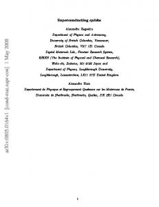
the need for tunable couplings, in contrast to earlier work [16, 17], and without restrictions on the number of and distance between physical qubits defining a given stabilizer operator. We thus extend the superconducting qubit toolbox with functionality similar to that recently demonstrated for trapped ions [18]. Central to our proposal is the off-resonant coupling between a superconducting qubit and a single mode of a microwave resonator [19] described by the dispersive Hamiltonian Hdisp = χ σ z a† a, where σ z = |eihe| − |gihg| is the Pauli matrix in the computational basis {|gi, |ei} of the qubit and a (a† ) denotes the photon annihilation (creation) operator of the cavity mode. This coupling describes a qubit-state-dependent frequency shift ±χ of the cavity, or equivalently a photon-number-dependent frequency shift 2nχ of the qubit. In the weakly dispersive regime 2χ ∼ 1/T2 , κ, where κ is the bare cavity linewidth and T2−1 = (2T1 )−1 + Γφ is the qubit coherence time composed of relaxation 1/T1 and pure dephasing Γφ , this interaction enables a qubit-readout by measuring the phase-shift of transmitted or reflected microwaves [19]. In this work, we are interested in the ultrastrong dispersive regime of well-resolved resonances [20], where κ, T2−1 ≪ χ. In this regime, we show how to encode the two eigenvalues of an arbitrary multi-qubit Pauli operator onto quasi-classical oscillations of light that differ in phase by π. Although our scheme is applicable to other types of superconducting qubits, for clarity we will frame our discussion around the specific case of transmon qubits. A transmon qubit [21, 22] is formed by a superconducting dipole-antenna with a Josephson junction at its center with Josephson energy EJ ≫ EC ≡ e2 /(2CΣ ), where CΣ represents the total capacitance between the antenna pads. Neglecting charge-dispersion effects, which are suppressed exponentially in EJ /EC [21], the lowenergy spectrum of an isolated transmon is well approximated by that√ of an anharmonic oscillator with frequency ω01 ≈ 8EJ EC − EC and weak anharmonicity ω01 − ω12 ≈ EC ≪ ω01 . In state-of-the-art realizations, the qubit linewidth 1/T2 is close to being limited by relaxation [22–25]. In this work we are interested in a setup such as depicted in Fig. 1 (a), where N transmons are coupled dispersively with strength χ to a microwave field

2 (a) readout/reset cavity

readout (b) port 2N χ

2N χ

ω c − χA

ω c + χA

ω

transmon qubit

ancilla qubit

Josephson Junction

(c)

~ E

0 1 ωqi ωqi

drive port

√ ¯χ 2 n

2χ

1 0 ωqi+1 ωqi+1

ω

FIG. 1. (Color online) (a) 2D array of N transmon qubits in a 3D cavity. The ancilla qubit and the upper cavity are used for readout/reset and manipulation purposes. Cavity (b) and qubit (c) spectra in the ultra-strong dispersive regime.

inside a 3D cavity. For simplicity, we here discuss the case of equal dispersive couplings. In the supplemental material we show how to cope with the more realistic case of unequal dispersive shifts. For control and readout purposes, an ancilla qubit, is further dispersively coupled to both the high-Q cavity containing the N qubits with χA ≫ N χ and to a low-Q (readout) cavity, similar to the setup used in [26]. We assume that both the ancilla qubit and the readout cavity remain in the ground state, except during readout and manipulation. Thus omitting, for now, the corresponding degrees of freedom, we model this system in an appropriately rotating frame (see supplemental material for details), by the effective Hamiltonian H0 = χ

N X i=1

σiz a† a − Ka† a† aa .

(1)

The transmons are treated here as two-level systems assuming their anharmonicity is larger than their linewidth (i.e. EC > 1/T2 ). Furthermore, assuming the qubits to be sufficiently detuned from each other, we neglect the cavity-mediated qubit-qubit interaction. The latter leads to frequency shifts of the order of χ2 /∆, where ∆ is the detuning between the two qubits. For the parameters used below (χ = 5 MHz and ∆ ≥ 2 GHz), these shifts are smaller than about 10 KHz. The second term on the rhs of Eq. (1) accounts for the (negative) qubit-induced anharmonicity of the cavity [27, 28]. In the weak dispersive regime, this term can usually be neglected as K ≪ χ. We find that in the ultra-strong dispersive regime it is necessary to account for its leading order effect. next NN We z σ of an show how to encode the parity ZSN = i=1 i N -qubit state |ψiN onto two quasi-orthogonal coherent states of the cavity differing in phase by π. Parity encoding. Suppose the system is initially prepared in the product state |Ψit=0 = |αi|ψiN , where |αi is

a coherent state of the cavity with amplitude α. Making PN use of the identity exp[−i(π/2) i=1 σiz ] = (−i)N ZSN , one can show that under the action of (1), at time T = π/(2χ), the state becomes
|ΨiT = UK |αN iPS+N + |−αN iPS−N |ψiN , (2)

where PS±N = (11 ± ZSN )/2 are the projectors onto the even (+) and odd (−) qubit parity subspaces as measured by the ±1 eigenvalues of the multi-qubit Pauli operator ZSN and αN = (−i)N α. Note that the self-Kerr term is qubit-independent [29] and conserves the photon number a† a. Because it commutes with the dispersive term, its effect factors out and is captured in (2) by the unitary operator UK = exp[iπK/(2χ)a† a† aa]. For weak nonlinearity such that πK ≪ χ, the leading order effect of UK acting on the coherent states |±αN i is a rotation of the mean amplitude by an angle ∆φnl = π¯ nK/χ with the 2 mean photon number n ¯ = |α| . To leading order in K/χ, the state (2) is thus well approximated by ˜ N iPS−N |ψiN , |ΨiT = |˜ αN iPS+N |ψiN + |−α

(3)

with α ˜ N = αN e−i∆φnl . The sub-leading order effect is a damping of the mean amplitude by a factor exp(−∆φ2nl /(2¯ n)) [30]. We emphasize that in the ultrastrong dispersive regime κ/χ ≪ 1 considered here, photon decay only weakly damps the amplitude of the coherent states in (3) by a factor exp(−κT /2) ≈ 1 − (π/4)(κ/χ). Ignoring these small effects, we thus see that the dispersive interaction can be used to encode the parity of the multi-qubit state onto two coherent states of the cavity differing in phase by π. Subset selectivity. Typically stabilizer operators are defined on subsets of qubits. Selectivity to M ≤ N qubits, labeled by the set SM ⊆ SN = {1, . . . , N }, can be achieved as follows. Consider the identity USM (t) =

 O

i∈S / M

 t  O  t  σix USN , (4) σix USN 2 2 i∈S / M

P where US (t) = exp(−itχa† a i∈S σiz ). Eq. (4) can be easily shown using σ x σ z σ x = −σ z . Thus, by splitting the dispersive evolution of all N qubits into two equal halves and interspersing them with bit-flip operations on the qubits not in SM , we can effectively echo away the contribution of the latter to the total “magnetization” and implement the dispersive evolution USM (t) of the qubits in SM alone. Acting on an initial state of (T = π/(2χ)) then encodes the the form |αi|ψiN , USMN z subset-parity ZSM = i∈SM σi onto the state of the cavity as explained above. The case of unequal dispersive shifts is treated in the supplemental material. Physically, the initial unconditional cavity displacement and bit-flips can be implemented via fast microwave pulses (see supplemental material). Because

3 of the dispersive interaction, the qubit transition frequency of the i-th qubit splits into a ladder of frequencies n 0 ωqi = ωqi + 2nχ, corresponding to different photon numbers in the cavity (Fig. 1 (c)). The latter are Poisson distributed and peaked around n ¯ . Hence, to best approximate an unconditional rotation of the i-th qubit, 0 the pulse must be centered at the frequency ωqi + 2¯ nχ √ ¯ χ. and have a frequency-width large compared with 2 n For |α| ≥ 1/π √ the duration of such a π-pulse is thus Tπ ≪ 1/(2 n ¯ χ) ≤ T . Similarly, the initial coherent state of the cavity |αi can be prepared from the vacuum by driving the cavity at the frequency ωc − χA with a pulse of area α and a frequency-width large compared with 2N χ; the maximal frequency spread of a cavity dispersively coupled with strength χ to N qubits (Fig. 1 (b)). Again the duration Td of this pulse is short since Td ≪ 1/(2N χ) < T . The total duration of the encoding is thus dominated by the dispersive evolution time T = π/(2χ), which is independent of N and M .

(a)

|0ic 1 |ψi4 2 3 4

(b)

0.

0.

1.

Dα

πx T1/2

1. 2.

T1/2

πx 2.

3. 3.

4. 4.

N tor QSM = i∈S τi , with τi ∈ {σix , σiy , σiz }. M Parity readout. The encoded state is of the form ˜ M iPS−M |ψiN , where PS±M = |ΨiT = |˜ αM iPS+M |ψiN + |−α ˜ M = (−i)M e−i∆φnl α. The overlap be(11±QSM )/2 and α tween the two cavity states, h˜ αM | − α ˜ M i = exp(−2|α|2 ), is independent of K and M . For large |α|, these two states are distinguishable in principle and a measurement of the cavity state is equivalent to a multi-qubit parity measurement. A fast readout of the cavity state with Tmeas ≪ 1/κ, may be achieved by lowering the Q-factor of the cavity containing the qubits (κ → κ′ ≫ κ), as recently demonstrated [31]. This Q-switching adversely affects the lifetime of the qubits via the Purcell effect. However, the latter is expected to be weak as long as κ′ ≪ χ. Alternatively, the cavity state can be mapped onto the ancilla qubit, which can subsequently be measured through standard homodyne measurement of the low-Q readout cavity. The mapping is achieved physically in three steps. First, the high-Q cavity field is displaced unconditionally by α ˜ M . To a good approximation, this maps the encoded state onto

πx

Dα˜ M |ΨiT = |2α ˜ M iPS+M |ψiN + |0iPS−M |ψiN .

πx

The second step consists in performing a π-pulse on the ancilla qubit, which so far was in its ground state, conditioned on the cavity being in the vacuum state. As first proposed in [32] and demonstrated in [26], this can be achieved by applying a pulse centered on the bare ancilla qubit transition frequency, which is narrow in frequency compared with 8¯ nχA (the additional factor of 4 is due to the twice as large amplitude of the cavity state in the first term on the rhs of Eq. (5)). Because χA ≫ N χ, a pulse duration TA can be chosen such that 1/(2χA ) ≪ TA ≪ 1/(2N χ). For n ¯ > 1/4 the first inequality guarantees conditionality while the second one allows us to neglect the dispersive evolution during this operation. The state then becomes approximately     |2α ˜ M i PS+M |ψiN |giA + |0i PS−M |ψiN |eiA . (6)

5. 5.

α ˜

−α ˜ FIG. 2. (Color online) (a) Quantum circuit diagram for encoding the parity of qubits 2 and 4 (full (blue) lines). Dα represents the displacement operation, πx a single-qubit πpulse and T1/2 a free dispersive evolution of duration π/(4χ). (b) Numerical simulation of the evolution of the Q-function of the cavity [30], with an initial qubit state |ψi4 = (|gggei + √ |ggegi + |eeegi)/ 3. Dissipation from photon loss at a rate κ/(2π) = 10 KHz and qubit decoherence with T1 = T2 = 20 µs are included as well as a finite displacement and π-pulse duration of 1 ns. Other parameters are: α = 2, χ/(2π) = 5 MHz and K/(2π) = 80 KHz. The self-Kerr term leads to an additional phase rotation ∆φnl = 2K n ¯ ∆t, where ∆t = 50.3 ns is the total duration of the encoding. Taking this rotation into account, we obtain a fidelity of F = 98% to the ideal target − + |ψi4 . |ψi4 + |−α ˜ 2 iP{2,4} state |Ψiideal = |α ˜ 2 iP{2,4}

As an example, Fig. 2 shows the results of a numerical simulation encoding the parity of M = 2 out of N = 4 qubits, which accounts for finite (square) pulse duration, decoherence and qubit-induced cavity nonlinearity. For the parameter values given in the caption, we find a fidelity (overlap with the ideal target state) of 98%. By applying single-qubit rotations to individual qubits before and after the encoding one may similarly encode the parity of an arbitrary weight M Pauli opera-

(5)

In the third and final step, a displacement of −2α ˜M is performed on the cavity conditioned on the ancilla qubit being in the ground state. This is achieved with a pulse centered at frequency ωc − χA , with a frequencywidth small compared with 2χA but large compared with 2N χ. Neglecting again the dispersive evolution during this step, the state finally becomes h    i |0i PS+M |ψiN |giA + PS−M |ψiN |eiA . (7)

Note that the state (7) is now stationary with respect to the dispersive interaction, there being no photons in the cavity. Reading out the state of the ancilla qubit amounts to measuring QSM . After the measurement, the ancilla qubit may be reset to the ground state efficiently via the readout cavity [33].

4 1.0e-01

(8)

Note that χA ≫ N χ guarantees that the adiabatic condition wrt χA can be satisfied while still remaining fast wrt the dispersive time scale 1/(N χ). In (8) we omitted the state of the ancilla qubit, since it starts and ends in the ground state and thus factors out. The cavity is disentangled from the state by applying the encoding protocol with α replaced by −α ˜ M . After unconditionally displacing the cavity back to the vacuum, taking into account an additional nonlinear phase acquired during the decoding, the N -qubit state finally becomes PS+M |ψiN + e2iθ PS−M |ψiN = eiθ e−iθQSM |ψiN ,

(9)

which up to an unimportant global phase factor, represents the action of the desired unitary. Application. To test the feasibility of the above protocols, we simulated the preparation of a logical qubit state of the four-qubit erasure channel code [34]. The stabilizer generators of this code are S = {Z1 Z2 , Z3 Z4 , X1 X2 X3 X4 }, where we have switched to the standard notation Xi and Zi for the Pauli operators of qubit i. The code-space is spanned by the two +1 eigenstates of the stabilizer operators: |±i =

1 (|ggi ± |eei)(|ggi ± |eei). 2

(10)

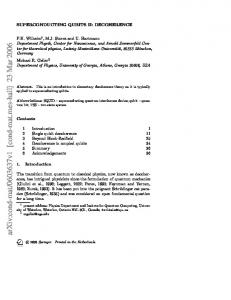
The logical qubit Pauli operators are Z = X1 X2 = X3 X4 and X = Z1 Z3 = Z2 Z4 = Z1 Z4 = Z2 Z3 . Because of the redundancy of the logical operators, this code protects a logical qubit state α|+i+β|−i from the loss (i.e. arbitrary error) of a known qubit [34]. Here we prepare the logical qubit state ψ = exp[−i(π/8)X]|+i as follows. (i) We start with the fully polarized four-qubit state |ggggi, which is already a +1 eigenstate of the Z stabilizer operators. (ii) Using the encoding protocol, we measure the logical Z operator X1 X2 . If we obtain −1, we apply Z1 . (iii) We measure the operator X3 X4 . If we obtain −1 we apply Z3 . (iv) We reset the cavity to the vacuum. These four steps prepare the logical state |+i. We next use the ancilla (with χA = 10N χ) to implement the rotation as described above with QS4 = X and θ = π/8. Fig. 3 shows the obtained fidelity to the ideal target state

κT6.8e-03

1.0e-02

5.1e-03

4.1e-03

0.94

0.80

30 25

Fqb

0.67

20

0.54

15 10

0.40 5 0

|2α ˜ M iPS+M |ψiN + e2iθ |0iPS−M |ψiN .

2.0e-02

35

K/κ

Simulated time evolution. The ancilla qubit can also be used to simulate the “time evolution” exp[−iθQSM ] under the action of an arbitrary Pauli operator QSM . This is useful e.g. for manipulating a logical qubit state encoded in a stabilizer subspace in which case QSM is taken to be a logical qubit Pauli operator. Starting from the state Eq. (5), this is achieved by adiabatically driving the ancilla around a closed loop on its Bloch sphere subtending a solid angle 4θ, conditioned on there being no photons in the cavity. The component in Eq. (5) with zero photons then acquires a phase of 2θ (half the solid angle) and the state becomes

200

400

600

χ/κ

800

1000

0.27

FIG. 3. (Color online) Fidelity of the prepared state to exp[−i(π/8)X]|+i. The (red) dashed curve represents the boundary of the inequality K ≥ χ2 /(4αq ) which relates the self-Kerr K with the dispersive shift χ and the single-qubit anharmonicity αq [27]. Here αq /(2π) = 200 MHz.

exp[−i(π/8)X]|+i as a function of χ and K in units of κ/(2π) = 10 KHz and for T1 = T2 = 20 µs. The total duration T of the state preparation is shown on the upper x-axis in units of 1/κ. Focusing on the line K = 0, when χ is small T is large and dominated by the dispersive evolutions and the fidelity is limited by a combination of qubit decoherence, photon loss and faulty conditional ancilla rotation. The fidelity then increases with increasing χ, which reduces the preparation time T and hence the effects of decoherence and improves the fidelity of the conditional ancilla rotation. It reaches a maximum in a regime where both conditional and unconditional operations can be performed with high fidelity. A further increase in χ degrades the unconditional cavity displacement and qubit rotations (a 1 ns pulse corresponds to a width of ∼ 160 MHz) and the fidelity drops. The cavity nonlinearity K and the dispersive shift χ are in fact not independent, but rather related via the single-qubit anharmonicity αq , by the inequality K ≥ χ2 /(4αq ) [27], which is shown as a dashed (red) curve in Fig. 3 for αq /(2π) = 200 MHz. In conclusion, we proposed a protocol to measure stabilizer operators defined on an arbitrary subset of superconducting qubits in the ultra-strong dispersive regime of cQED. Challenges for the future will be to extend the present protocol to carry out multiple stabilizer measurements in parallel and to make it scalable perhaps by using multiple cavities as in [14] and an efficient encoding of multiple bits of information onto the photonic Hilbert space [32]. We thank L. Jiang, M. Mirrahimi, D. Poulin, M. Devoret and R. Schoelkopf for discussions. The simulations were coded in Python using the QuTip library [35]. This work was supported by the Swiss NSF, the NSF (DMR1004406) and the ARO (W911NF-09-1-0514).

5

[1] M. Ansmann, H. Wang, R. C. Bialczak, M. Hofheinz, E. Lucero, M. Neeley, A. D. O’Connell, D. Sank, M. Weides, J. Wenner, A. N. Cleland, and J. M. Martinis, Nature 461, 504 (2009). [2] M. D. Reed, L. DiCarlo, S. E. Nigg, L. Sun, L. Frunzio, S. M. Girvin, and R. J. Schoelkopf, Nature 482, 382 (2012). [3] D. Gottesman, Stabilizer Codes and Quantum Error Correction, Ph.D. thesis, Caltech (1997). [4] D. J. C. MacKay, G. Mitchison, and P. L. McFadden, IEEE Transactions on Information Theory 50, 2315 (2004); A. A. Kovalev and L. P. Pryadko, “Quantum ”hyperbicycle” low-density parity check codes with finite rate,” (2013), arXiv:quant-ph/1212.6703v2. [5] A. Kitaev, Annals of Physics 303, 2 (2003). [6] S. Bravyi and A. Kitaev, “Quantum codes on a lattice with boundary,” (1998), arXiv:quant-ph/9811052. [7] D. S. Wang, A. G. Fowler, A. M. Stephens, and L. C. L. Hollenberg, Quantum Information & Computation 10, 456 (2010); A. G. Fowler, M. Mariantoni, J. M. Martinis, and A. N. Cleland, Phys. Rev. A 86, 032324 (2012). [8] E. Dennis, A. Kitaev, A. Landahl, and J. Preskill, Journal of Mathematical Physics 43, 4452 (2002). [9] O. Landon-Cardinal and D. Poulin, Phys. Rev. Lett. 110, 090502 (2013). [10] S. Chesi, B. R¨ othlisberger, and D. Loss, Phys. Rev. A 82, 022305 (2010). [11] A. Hutter, J. R. Wootton, B. R¨ othlisberger, and D. Loss, Phys. Rev. A 86, 052340 (2012). [12] R. Alicki, M. Horodecki, P. Horodecki, and R. Horodecki, Open Systems & Information Dynamics 17, 1 (2010). [13] K. Lalumi`ere, J. M. Gambetta, and A. Blais, Phys. Rev. A 81, 040301 (2010). [14] D. P. DiVincenzo and F. Solgun, (2012), arXiv:1205.1910 [quant-ph]. [15] T. Tanamoto, V. M. Stojanovic, C. Bruder, and D. Becker, (2013), arXiv:1301.4796 [quant-ph]. [16] T. P. Spiller, K. Nemoto, S. L. Braunstein, W. J. Munro, P. van Loock, and G. J. Milburn, New Journal of Physics 8, 30 (2006). [17] C. R. Myers, M. Silva, K. Nemoto, and W. J. Munro, Phys. Rev. A 76, 012303 (2007). [18] J. T. Barreiro, M. M¨ uller, P. Schindler, D. Nigg, T. Monz, M. Chwalla, M. Hennrich, C. F. Roos, P. Zoller, and R. Blatt, Nature 470, 486 (2011); M. M¨ uller, K. Hammerer, Y. L. Zhou, C. F. Roos, and P. Zoller, New. J. Phys. 13, 085007 (2011). [19] A. Blais, R.-S. Huang, A. Wallraff, S. M. Girvin, and R. J. Schoelkopf, Phys. Rev. A 69, 062320 (2004). [20] D. I. Schuster, A. A. Houck, J. A. Schreier, A. Wallraff, J. M. Gambetta, A. Blais, L. Frunzio1, J. Majer, B. Johnson, M. H. Devoret, S. M. Girvin, and R. J. Schoelkopf, Nature 445, 515 (2007). [21] J. Koch, T. M. Yu, J. Gambetta, A. A. Houck, D. I. Schuster, J. Majer, A. Blais, M. H. Devoret, S. M. Girvin, and R. J. Schoelkopf, Phys. Rev. A 76, 042319 (2007). [22] H. Paik, D. I. Schuster, L. S. Bishop, G. Kirchmair, G. Catelani, A. P. Sears, B. R. Johnson, M. J. Reagor, L. Frunzio, L. I. Glazman, S. M. Girvin, M. H. Devoret, and R. J. Schoelkopf, Phys. Rev. Lett. 107, 240501 (2011).

[23] M. Lenander, H. Wang, R. C. Bialczak, E. Lucero, M. Mariantoni, M. Neeley, A. D. O’Connell, D. Sank, M. Weides, J. Wenner, T. Yamamoto, Y. Yin, J. Zhao, A. N. Cleland, and J. M. Martinis, Phys. Rev. B 84, 024501 (2011). [24] G. Catelani, R. J. Schoelkopf, M. H. Devoret, and L. I. Glazman, Phys. Rev. B 84, 064517 (2011). [25] G. Catelani, S. E. Nigg, S. M. Girvin, R. J. Schoelkopf, and L. I. Glazman, Phys. Rev. B 86, 184514 (2012). [26] G. Kirchmair, B. Vlastakis, Z. Leghtas, S. E. Nigg, H. Paik, E. Ginossar, M. Mirrahimi, L. Frunzio, S. M. Girvin, and R. J. Schoelkopf, Nature 495, 205 (2013). [27] S. E. Nigg, H. Paik, B. Vlastakis, G. Kirchmair, S. Shankar, L. Frunzio, M. H. Devoret, R. J. Schoelkopf, and S. M. Girvin, Phys. Rev. Lett. 108, 240502 (2012). [28] J. Bourassa, F. Beaudoin, J. M. Gambetta, and A. Blais, Phys. Rev. A 86, 013814 (2012). [29] Qubit-state-dependent corrections to the self-Kerr are of order ϕ ˆ6 in an expansion of the Josephson potential p EJ cos(ϕ) ˆ and are smaller by a factor ∼ EC /EJ . [30] D. F. Walls and G. J. Milburn, Quantum optics, 2nd ed. (Springer, 2008). [31] Y. Yin, Y. Chen, D. Sank, P. J. J. O’Malley, T. C. White, R. Barends, J. Kelly, E. Lucero, M. Mariantoni, A. Megrant, C. Neill, A. Vainsencher, J. Wenner, A. N. Korotkov, A. N. Cleland, and J. M. Martinis, (2012), arXiv:1208.2950 [cond-mat]. [32] Z. Leghtas, G. Kirchmair, B. Vlastakis, M. H. Devoret, R. J. Schoelkopf, and M. Mirrahimi, Phys. Rev. A 87, 042315 (2013). [33] K. Geerlings, Z. Leghtas, I. M. Pop, S. Shankar, L. Frunzio, R. J. Schoelkopf, M. Mirrahimi, and M. H. Devoret, (2012), arXiv:1211.0491 [cond-mat.mes-hall]. [34] M. Grassl, T. Beth, and T. Pellizzari, Phys. Rev. A 56, 33 (1997). [35] J. Johansson, P. Nation, and F. Nori, Computer Physics Communications 183, 1760 (2012). [36] A derivation which goes beyond this simple dipole approximation to include the exact linear normal modes is given in [27, 28]. [37] We also neglect multi-photon processes. [38] M. Boissonneault, J. M. Gambetta, and A. Blais, Phys. Rev. Lett. 105, 100504 (2010). [39] H.-P. Breuer and F. Petruccione, The theory of open quantum systems (Oxford Univ. Press, 2007). [40] R. Raussendorf and H. J. Briegel, Phys. Rev. Lett. 86, 5188 (2001). [41] R. Raussendorf, D. E. Browne, and H. J. Briegel, Phys. Rev. A 68, 022312 (2003).

6

Supplemental Material for “Stabilizer quantum error correction toolbox for superconducting qubits” Simon E. Nigg and S. M. Girvin Departments of Physics, Yale University, New Haven, CT 06520, USA (Dated: May 6, 2013) In these notes, we derive the effective Hamiltonian of Eq. (1) in the main text. We generalize the subset parity encoding to arbitrary dispersive shifts. We calculate finite pulse-width effects for the unconditional displacement and single-qubit rotations and discuss the constraints imposed on the drive and system spectrum. We describe a modification of the parity measurement protocol for stabilizer pumping. We briefly discuss our treatment of decoherence and present the state tomography of the encoded logical qubit state of the erasure code. Finally we conclude with a discussion of possible applications and extensions.

DERIVATION OF THE EFFECTIVE MODEL OF EQ. (1)

In terms of its two conjugate variables ϕ and n, which represent the superconducting phase difference and the number of Cooper pairs transferred across the Josephson junction (JJ), a transmon qubit is conventionally described by the Hamiltonian [21] H = 4EC (n − ng )2 + EJ (1 − cos(ϕ)) = 4EC (n − ng )2 +

EJ 2 ϕ + Vnl (ϕ) . 2

(11)

In the second equality we have explicitly separated the harmonic and anharmonic parts of the Josephson potential EJ (1 − cos(ϕ)) = ϕ2 EJ /2 + Vnl (ϕ). For EJ ≫ EC , the “phase particle” essentially undergoes quasi-harmonic oscillations around a local minimum of the cosine potential, with rare 2π quantum phase-slip events, which lead to a weak (exponentially suppressed in EJ /EC ) dependence of the energy levels on the offset charge ng [21]. In the following we will neglect the latter and set ng = 0. p It is convenient to diagonalize the√harmonic part by introducing p the bare mode operator a0 = EJ /(2~ω0 ) ϕ + 2i EC /(~ω0 ) n and frequency ~ω0 = 8EJ EC . Then expanding the non-linear potential to leading order (ϕ4 ) one obtains H = ~ω0 (a†0 a0 + 1/2) −

EC (a0 + a†0 )4 + O(ϕ6 ) 12

(12)

p Note that the coefficient of a given term in the expansion is smaller than the previous one by a factor ∼ p EC /EJ . We are primarily interested in low-lying energy levels, for which the wavefunctions are localized in phase i.e. hϕ2 i ≪ π. Hence we consider here only the leading order ϕ4 non-linearity. The coupling of a transmon with the electromagnetic field of a resonator is typically described in the dipole P approximation [36] by a term ∼ n · E where E = k iǫk (bk − b†k ) is the quantized electric field of the (multi-mode) resonator written in terms of its eigenmodes bk . In a straightforward generalization of the above, the Hamiltonian of Nqb transmons coupled to multiple harmonic modes can be written in the general form (suppressing from now on the zero-point energies) v u qb Nqb Nqb X X X X u ǫ j t ~ωi (i) † † qb † c † Vnl (ϕi ) with gij = gij (ai − ai )(bj − bj ) + ~ωj bj bj + ~ωi ai ai + H= (13) (i) 2 E i=1 ij j i=1 C

(i)

(i)

Here Vnl (ϕi ) = EJ [(1 − cos(ϕi )) − ϕi 2 /2]. As before, it is convenient to diagonalize the harmonic part. As shown in [27], this diagonalization can be achieved from the knowledge of the Nqb × Nqb impedance matrix Z of the corresponding linearized circuit with each one of the Nqb JJs representing a port. Denoting the normal modes by cp and their frequencies by ωp , one obtains explicitly (k) ϕi

=

φ−1 0

M X Zik (ωp ) Z kk (ωp ) p=1

r

~ eff Z (cp + c†p ) with 2 kp

eff Zkp =

2 ωp Im[∂ω Yk (ωp )]

(14)

7 Here φ0 = ~/(2e) is the reduced flux quantum and we have introduced the admittance at port k defined as Yk = 1/Zkk . The choice of the port k is arbitrary and reflects a particular basis choice. The total number of modes is denoted by M . The mode frequencies ωp are given by the zeros of the imaginary part of the admittance, i.e. ImYk (ωp ) = 0 (note that in the dissipationless case, the elements of Z are purely imaginary). Keeping the leading order ϕ4 non-linearity and normal-ordering the latter, the Hamiltonian of the system then takes the form   X X (15) H4 = ωp c†p cp − γpp′ 2c†p cp′ + c†p c†p′ + cp cp′ p

−

X

pp′

pp′ qq′

  βpp′ qq′ 6c†p c†p′ cq cq′ + 4c†p c†p′ c†q cq′ + 4c†p cp′ cq cq′ + cp cp′ cq cq′ + c†p c†p′ c†q c†q′ ,

with βpp′ qq′ = R0−2

Nqb (i) q X EJ Zik (ωp ) Zik (ωp′ ) Zik (ωq ) Zik (ωq′ ) eff Z eff Z eff Z eff Zkp ′ ′ kp kq kq 6 Zkk (ωp ) Zkk (ωp′ ) Zkk (ωq ) Zkk (ωq′ ) i=1

(16)

P where R0 = ~/e2 and γpp′ = 6 q βqqpp′ . Eqs. (15) and (16) together with a model for the impedance matrix, allow one to design the circuit Hamiltonian [27, 28]. Importantly, the above derivation provides the functional dependence among the parameters ωp , γp′ and βpp′ qq′ . By applying a generalized RWA in the dispersive limit of large detuning between the modes [37], we may neglect rapidly-rotating and non-diagonal terms and thus consider the simplified form X 1X χpq c†p c†q cq cp Heff = ωp′ c†p cp + (17) 2 pq p where we have defined χpq = −24βpqqp for q 6= p and χpp = −12βpppp . The frequencies have been renormalized as ωp′ = ωp − 2γpp . The second term on the rhs of (17) describes self-Kerr (χpp ) and cross-Kerr (χqp with q 6= p) interactions between the modes. From the Cauchy-Schwarz inequality and Eq. (16), it can be shown that χ2qp ≤ 4χqq χpp ; equality holding in the single-qubit case. In the dispersive regime of interest here, the hybridization of qubit and cavity modes is small and one can unambiguously identify the qubit-like modes as those with the strongest anharmonicities. Assuming the latter are much larger than the linewidth and as long as the drive frequencies used are different from transitions between the first and second excited states, the qubit Hilbert space can be truncated to the lowest two levels. From (17) we then obtain, denoting the cavity modes with ai and suppressing constant terms H0 =

Nqb qb X ω i

i=1

2

σiz +

X

ωjc a†j aj +

Nqb X X i=1

j

j

χij σiz a†j aj −

X

Ki a†i a†i ai ai ,

(18)

i

where Ki ≡ χii and we have kept only the dispersive and qubit-cavity cross-Kerr shifts. We note that in addition to these interaction terms there exist in general also qubit-qubit (∼ σiz σjz , i 6= j) and cavity-cavity (∼ a†i ai a†j aj , i 6= j) cross-Kerr shifts. However in the regime of interest here, the coefficients of these terms are small and will consequently be neglected. A qubit-induced cavity non-linearity has previously been derived within the dispersive approximation of a multilevel generalization of the Tavis-Cummings model [38]. In addition to the qubit independent term discussed here, such a treatment also yields qubit dependent non-linearities. In our derivation, qubit dependent self-Kerr terms appear only at order ϕ6 and higher and are parametrically small for large ratios EJ /EC . We can now apply (18) to our system depicted in Fig. 1 of the main text. From the above derivation, we see that in principle all qubits (N active qubits and 1 ancilla qubit) couple to multiple modes of both cavities. However, in the weakly coupled dispersive limit for the readout cavity and appropriately chosen parameters, we may neglect the coupling of the active qubits with the readout (low-Q) cavity mode and higher modes of the active (high-Q) cavity. Similarly the ancilla approximately only couples to a single mode in each cavity. Denoting the dispersive shift of the N qubits by χi and that of the ancilla with the active cavity mode a by χA ≫ N χ and with the readout cavity mode b by χ′A we obtain H0 =

N X ω qb i

i=1

2

σiz + ωc a† a +

N X i=1

χi σiz a† a + χA σzA a† a − Ka† a† aa + Hreadout ,

(19)

8 with Hreadout = ωc′ b† b + χ′A σzA b† b h− K ′b† b† bb. Finally, moving to a frame i rotating with qubits and cavity by the P qb z † χ unitary transformation U (t) = exp −it yields: i (ωi /2)σi + (ωc − A )a a H0 =

N X i=1

χi σiz a† a − Ka† a† aa ,

(20)

which for equal dispersive shifts χi = χ reduces to Eq. (1) of the main text. This model is a valid when the ancilla qubit and readout cavity remain in their ground state, in which case Hreadout = 0. FINITE PULSE-WIDTH EFFECTS ON UNCONDITIONAL OPERATIONS

Having motivated the form of our Hamiltonian (20) [Eq. (1) of the main text], we here use it to investigate the effects due to finite pulse-width when driving the system with simple realistic pulses. To distinguish these effects from the nonlinear effects we here set K = 0. In the following discussion, we concentrate on the unconditional operations necessary for the parity encoding protocol and neglect the ancilla qubit and readout cavity. Pulse duration constraints for the conditional pulses are discussed in [32]. We further assume independent drives for the qubits and the cavity mode. For the latter to be a valid approximation, the qubits need to be sufficiently detuned from each other and from the cavity. In the rotating frame of Eq. (20), a cavity drive at frequency ωd is then described by Hdc (t) = ε0 (t)(eit(ωc −

χA −ωd )

a† + h.c.).

(21)

In the same rotating frame, a simultaneous drive of the qubits in a set S ∈ SN = {1, . . . , N } at frequencies ωid for i ∈ S, is described by a term Hdqb (t) =

X Ωi (t) 2

i∈S

qb

(σi+ eit(ωi

−ωid )

+ h.c.).

(22)

Unconditional displacement

At the start of the encoding, we need to be able to displace the cavity from the vacuum into a coherent state with amplitude α independently of the state of the qubits. We choose ωd = ωc − χA and consider the Hamiltonian ! N X z σi a† a + ε0 (t)(a + a† ). (23) H(t) = χ i=1

Let us denote the computational basis states of N qubits by |i1 , . . . , iN i, with σjz |iP j i = ij |ij i and ij ∈ {−1, 1}. Under the action of the Hamiltonian (23), the initial product state |0ic |ψiN with |ψiN = i1 ,...,iN ci1 ,...,iN |i1 , . . . , iN i evolves into Z t  X iχ(τ −t)Ai1 ,...,iN |i1 , . . . , iN i, (24) ci1 ,...,iN −i dτ ε0 (τ )e |ψ(t)i = 0

i1 ,...,iN

PN where Ai1 ,...,iN = j=1 ij . For simplicity, we consider a square pulse with envelope ε0 (t) = ǫ0 θ(T − t). The amplitude of the coherent state associated with the qubit component |i1 , . . . , iN i at time T becomes αT = −iǫ0 T e−

χAi1 ,...,iN T

i

2

sinc (χAi1 ,...,iN T /2) ,

(25)

where sinc(x) = sin(x)/x. Thus there is both a qubit-state dependent rotation and a suppression of the amplitude of the coherent state. Since −N ≤ Ai1 ,...,iN ≤ N , if N χT ≪ 1, we can expand and obtain αT = −iǫ0 T − ǫ0 T 2 χ

Ai1 ,...,iN + O((N χT )2 ). 2

(26)

9 Thus the first-order correction to the displacement of the cavity state is a qubit-state dependent rotation. The change in amplitude is second order in N χT . This has important consequences for the encoding protocol, since it allows for a partial compensation of the finite pulse-length effect of the displacement simply by shortening the duration of the subsequent free evolution part. Retaining only the leading order term, the state in (24) factorizes and we have |ψ(T )i ≈ |−iǫ0 T i|ψiN .

(27)

which corresponds to a cavity displaced by α = −iǫ0 T , while the qubits were left unchanged. In terms of the drive strength and final coherent state amplitude, this is valid when |α| ≪ ǫ0 /(N χ). Because −N ≤ Ai1 ,...,iN ≤ N , the maximum amplitude difference is given to first order by ǫ0 T 2 N χ = |α|N χT . We may then define a fidelity of the displacement operation as the absolute value of the overlap between an ideally displaced coherent state and a state with maximal phase difference. To leading order, this is found to be   1 2 F ≈ exp − (|α|T χ) . (28) 8 Thus we see that to achieve high fidelity, the average number of photons in the cavity n ¯ = |α|2 should satisfy √ χ n ¯ N T ≪ 8. Fig. 4 shows the numerically computed fidelity to the target displaced state obtained from the initial state |0ic |ggggi as a function of the square pulse duration T . For this simulation we took χ/(2π) = 10 MHz, α = 2.5.

1.0

0.9

0.8

F

0.7

0.6

0.5

0.4

0.3

0.2

0.2

0.4

NχT/π

0.6

0.8

1.0

FIG. 4. Fidelity of un-conditional displacement for the initial state |0ic |ggggiN=4 as a function of square pulse duration T . The dashed (red) curve shows F = exp[−(|α|N χT )2 /8]. We took a dispersive shift χ/(2π) = 10 MHz, and a cavity displacement α = 2.5.

Unconditional qubit selective π-pulses

In order to perform subset-selective parity measurements, one needs to perform unconditional π-pulses on subsets of qubits as explained in the main text. Following the discussion in the main text we choose the drive frequencies to be ωid = ωiqb + 2¯ nχ and thus consider the following Hamiltonian in the rotating frame ! N  X Ωj (t)  X χ z σi a† a + H(t) = χ e2i¯n t σj− + h.c. . (29) 2 c i=1 j∈SM

Note that here we have neglected the off-resonant driving of the qubits in SM . In order √ for this to be valid, we must ¯ χ, such that we may find a require the frequency detuning between any two qubits to be large compared with 2 n

10 √ c pulse duration T satisfying |ωqi − ωqj |i6=j ≫ T −1 ≫ 2 n ¯ χ. Moving to a frame rotating with the qubits in SM at frequency n ¯ χ, we can write the Hamiltonian as (we use the same symbol H to denote the Hamiltonian in the new frame)     X X X Ωj (t) σjx . (30) H = χ σjz  a† a + χ  σjz  (a† a − n ¯) + 2 c c j∈SM

j∈SM

j∈SM

Clearly the first term on the rhs commutes with the remaining terms and leads to a “free” evolution of the qubits in P SM and of the cavity given by USM (t) = exp(−itχa† a i∈SM σiz ). The action of the last two terms on each qubit in c SM is described by a single qubit Hamiltonian of the form H1 = χσ z (a† a − n ¯) + Defining β(t) =

Rt 0

Ω(τ ) 2 dτ ,

Ω(t) x σ . 2

(31)

the associated evolution operator is

Rt z 2 2 y x χ † U1 (t) = e−iβ(t)σ e−i (a a−¯n) 0 dτ {σ [cos (β(τ ))−sin (β(τ ))]+2σ sin(β(τ )) cos(β(τ ))}.

(32)

For χ = 0 this reduces to a simple σ x rotation, the angle of which is determined by the integral of the pulse envelope. The total evolution operator, including the contribution from the first term on the rhs of (30), is then U (t) = USM (t)e

−iβ(t)

P

j∈S c M

σjx −iχ(a† a−¯ n)

e

P

j∈S c M

Rt 0

dτ {σjz [cos2 (β(τ ))−sin2 (β(τ ))]+2σjy sin(β(τ )) cos(β(τ ))}

.

For a square pulse envelope Ω(t) = Ω0 θ(T − t) with T = π/Ω0 such that β(T ) = π/2 it is easy to show that   P P χ x π − iπ − 2i (a† a−¯ n) j∈S c σjy c σ M e 2 j∈SM j e Ω0 U (T ) = USM . Ω0

(33)

(34)

We are interested in the action of this operator on a coherent state or superposition √ of coherent states, for which the ¯ χ ≪ Ω0 , we have photon number is Poisson distributed around n ¯ with variance equal to n ¯ . Hence if 2 n     √ Y χ n ¯ T 2 . (35) U (T ) ≈ USM (T ) (−i)M σjx + O π j∈SM

If furthermore, we require that 2χM π ≪ Ω0 , then USM ≈ 11 + O(2χM T ) so that  √  Y 2 n ¯ χT U (T ) ≈ (−i)M σjx + O , 2χM T . π

(36)

j∈SM

Fig. 5 shows the fidelity as a function of the p square pulse duration T , of an unconditional two-qubit π rotation acting on an initial state |αic |ψi4 with |ψi4 = 1/3(|eeggi + |egggi − |eggei), α = 2.5 and for χ/(2π) = 10 MHz. Fidelity of subset selectivity

The infidelity of the displacement and π pulses, due to finite pulse duration discussed in the previous two sections, reduces the fidelity of the subset selectivity. To illustrate this, Fig. 6 shows the fidelity of the subset parity encoding of two out of four qubits discussed in the main text (See Fig. 2 in the main text), as a function of the displacement and π-pulse duration. As expected, the fidelity decreases monotonically with increasing pulse duration. As pointed out above, by reducing the duration of the free evolution periods, one can partially compensate for the finite duration of the displacement operation. This is illustrated by the full curve in Fig. 6, obtained by subtracting the displacement pulse duration from the free evolution periods. In contrast, the dashed curve shows the result without the correction. For the simulation we used square pulses and the same parameters (including dissipation and Kerr-nonlinearity) as in the main text. It is natural to expect that more sophisticated pulse shapes designed by optimal control techniques can be used to significantly improve the encoding fidelity, by suppressing the spectral weight at undesired frequencies.

11

1.1

1.0

F

0.9

0.8

0.7

0.6

0.5

0.02

0.04

0.06

0.08

nχT/π

0.10

0.12

0.14

FIG. 5. Fidelity of un-conditional π rotation of the first two qubits of the initial state |αic |ψi4 as a function of square pulse duration T . The cavity displacement is α = 2.5 and the dispersive shift is χ/(2π) = 10 MHz.

1.0 0.9 0.8

F

0.7 0.6 0.5 0.4 0.3 0.2 0

2

4

Tp (ns)

6

8

10

FIG. 6. Fidelity of subset parity encoding as a function of pulse duration. The parameters are the same as used in the example given in the main text. Full curve: encoding with shortened free evolution periods (Tfree → Tfree − Tp ). Dashed curve: encoding without adjustment of free evolution period.

SUBSET PARITY ENCODING FOR ARBITRARY DISPERSIVE SHIFTS

In the main text we discuss the case of equal dispersive shifts χi = χ. Although this could in principle be realized by fine tuning of the coupling strengths and detunings of the qubits with respect to the cavity mode, we here discuss a simple way to circumvent the need for tunability. This is advantageous since tunability invariably leads to shorter coherence times. For variable dispersive shifts, the main difference is that we now need to apply appropriately timed πpulses to all qubits. For simplicity we consider here instantaneous pulses and disregard the non-linear cavity self-Kerr

12 term. Thus we start from the dispersive interaction 

H0 = 

N X j=1

T



χj σjz  a† a.

(37)

T /2 t2 t1 t3

FIG. 7. Schematic representation of pulse sequence for arbitrary dispersive shifts. Each horizontal full line represents the time-line of a qubit the time origin being at the far right end. The vertical lines indicate the positions in time of bit-flips (pi-pulses).

As illustrated in Fig. 7, the idea is to use a pair of bit-flips for each qubit appropriately separated in time to adjust the cavity-phase contribution of each individual qubit. To simplify the discussion, let us label the M ≤ N qubits we wish to encode the parity of by the indices SM = {1, . . . M }. Denoting the total duration of the pulse sequence by T , the condition for qubit j ∈ SM to contribute to the encoded parity is χj (T − 2tj ) =

T π π , ⇔ tj = − 2 2 4χj

(38)

where tj ≤ T is the time delay between two bit-flips (applications of σjx ). To cancel the contribution to the total parity of the qubits not in SM it suffices to require that tj = T /2 for j ∈ / SM . Let us now further order the indices tj for j ∈ SM in order of increasing magnitude, i.e. 0 ≤ t1 ≤ t2 ≤ · · · ≤ tM ≤ T . The following operator then implements the desired subset-parity encoding     N N Y Y tM −tM −1 T −t T −tM t1 t2 −t1 t1 x −iH0 x x −iH0 2 M 2 e σM−1 . . . σ1x e−iH0 2  e . σjx  e−iH0 2 σ1x e−iH0 2 . . . σM UT =  σjx  e−iH0 2 σM j=M+1

j=M+1

(39)

Indeed, after some algebra one finds that UT =

Y

j∈SM

Y z † π z † χ e−i 2 σj a a . e−i j (T −2tj )σj a a =

(40)

j∈SM

Note that the time ordering used here is not unique and depending on the experimental conditions, a particular choice may be favored over others. Acting on a coherent state with amplitude α one finds + Y M z UT |αi = (−i) α σj , (41) j∈SM

which is the desired subset parity mapping. Note that the condition tj ≥ 0 implies that T ≥ π/(2 minj∈S (χj )). For χj = χ and T = π/(2χ) we recover the case discussed in the main text. STABILIZER PUMPING

In the main text we show how to measure a stabilizer by first encoding its eigenvalues onto the cavity state and then reading out the latter either directly or via the ancilla qubit and the readout cavity. Alternatively one can also

13 Q implement conditional jump operators of the form σix PS−M where PS±M = (11 ± ZSM )/2 with ZSM = i∈SM σiz and i ∈ SM . Such operators can be used to digitally simulate an artificial bath that pumps the system onto the stabilizer subspace as first proposed for trapped ions in [18]. The dissipative evolution under the action of such jump operators can be implemented with the protocol shown in Fig. 8. As for a parity measurement, one first encodes the eigenvalues of the parity operator onto the cavity state and applies and unconditional displacement to obtain the state (see Eq. (5) of the main text) |Ψi = |2α ˜ N iPS+M |ψiN + |0iPS−M |ψiN .

(42)

Instead of mapping the cavity state onto an ancilla as in the measurement protocol, one then applies a rotation by an angle θ around x of qubit i ∈ SM conditioned on the cavity being in the vacuum state. Note that this does not require an ancilla qubit. Because {σix , ZSM }+ = 0 for i ∈ SM , the state becomes PS+M (|ψiN |2αic + i sin(θ/2)σix |ψiN |0ic ) + cos(θ/2)PS−M |ψiN |0ic .

(43)

By resetting the cavity to the vacuum (via an ancilla qubit or a cavity Q-switch [31]) and repeating the procedure one generates the dissipative (non-unitary) evolution [18]   |0ih0| ⊗ ρN → |0ih0| ⊗ E0 (θ)ρN E0† (θ) + Ex(i) (θ)ρN Ex(i)† (θ) , (44) (i)

with E0 (θ) = PS+M + cos(θ/2)PS−M and Ex (θ) = i sin(θ/2)σix PS−M . Thus with probability sin2 (θ/2), a −1 eigenstate of ZSM is converted into a +1 eigenstate. For θ = π, this “stabilizer pumping” occurs with unit probability. Generalization to arbitrary weight-M Pauli-operators can be achieved with suitable single qubit rotations. |0ic 1 .. . .. .

Dα

Dα

T1/2

c Π SM

T1/2

c Π SM

•

reset|0ic

0 Xi∈S M ,θ

N FIG. 8. Quantum circuit diagram for stabilizer pumping. Dα denotes an unconditional displacement by α. T1/2 represents a c 0 c represents a (parallel) multi-qubit π-pulse on qubits in S free evolution of duration T1/2 = π/4χ. ΠSM M . Xi∈SM ,θ represents a conditional rotation of qubit i by θ around the x-axis, conditioned on the cavity being in the vacuum. reset|0ic represents the (dissipative) cavity reset operation.

DECOHERENCE

Decoherence due to photon losses and qubit decay and dephasing are treated within the Lindblad master equation formalism [39]. The master equation we solve numerically is  X  Γϕ D[σiz ]ρ + Γ− D[σi− ]ρ + Γ+ D[σi+ ]ρ , (45) ρ˙ = −i[H, ρ] + κD[a]ρ + 2 i where D[L]ρ = (2LρL† − L† Lρ − ρL† L)/2. Here κ is the single photon decay rate of the cavity, Γϕ is the phase relaxation (pure dephasing) rate of the qubits and the qubit relaxation rate is given by 1/T1 = Γ− + Γ+ . We consider the zero-temperature limit Γ+ = 0. LOGICAL QUBIT STATE TOMOGRAPHY

In Fig. 3 of the main text, we show the state fidelity of the encoded logical qubit state to the target state exp[−i(π/8)X]|+i as a function of the dispersive shift χ and cavity nonlinearity K. In the left panel of Fig. 9, we compare the resulting four-qubit state with the ideal target state in the Pauli-bar representation of the reduced

14 density matrix (tracing out the cavity), for K/(2π) = 80 KHz, χ/(2π) = 5 MHz and κ/(2π) = 10 KHz. The fidelity to the target state is 94%. The right panel of Fig. 9 shows the Bloch-sphere representation of the prepared logical qubit state. From the latter, we see that the infidelity is due to both a loss of purity and a deviation from the ideal rotation.

FIG. 9. (Color online) Left panel: Pauli-bar representation of the prepared four qubit state (full (blue) bars) and of the target state exp[−i(π/8)X]|+i (lighter (red) bars). Here P4 = {11, σ x , σ y , σ z }⊗4 is the Pauli-group of order four. Right panel: Bloch-sphere representation of the prepared logical qubit state (full (blue) vector) and corresponding target state (full (red) vector).

DISCUSSION & OUTLOOK

We conclude these notes by an informal discussion of a few possible applications of our protocol to illustrate its versatility.

Implementation of the toric code

Because we can measure Pauli operators on arbitrary subsets of qubits, it becomes possible to implement “in software” non-trivial topologies such as required e.g. by the toric code [5], in which 2g logical qubits can be encoded into the ground state stabilizer subspace of a qubit manifold with genus g. Let us consider the case g = 1 of a ring torus as depicted in Fig. 10. The stabilizers of the 2N -qubit toric code for example are the N plaquette Pi and N star operators Si defined as Pi =

Y

j∈plaquettei

σjz ,

Si =

Y

σjx .

(46)

j∈stari

Q Q Crucially, because of the toric boundary conditions it holds true that i∈lattice Pi = i∈lattice Si = 11. These two constraints then lead to a four-fold degeneracy (22g -fold degeneracy in general) of the ground state manifold. A ground state of the toric code can be prepared by starting from the fully polarized state |g, . . . , gi of the 2N qubits in the Z basis and sequentially measuring all the star operators and applying a corrective single qubit Z operation on a qubit in any star with eigenvalue −1. Fig. 10 illustrates a minimal 8-qubit toric code and its planar implementation.

15 (x)

5 4

Lh L(z) h 3

6

(z)

5 1

2

7

3

4

1

7

2

6 Lv (x) Lv 8

8

FIG. 10. Left panel. 8-qubit toric code. The qubits are represented by read beads. Right panel. Corresponding planar representation. The latter is easier to implement experimentally and the toric boundary conditions are imposed when defining (j) the stabilizers. Li indicate the incontractible loops used to define the logical qubit operators (see text).

The stabilizers of this code are explicitly: P1 = Z1 Z4 Z7 Z8 P2 = Z2 Z3 Z7 Z8

S 1 = X1 X2 X5 X7 S 2 = X3 X4 X5 X7

P3 = Z1 Z4 Z5 Z6

S 3 = X1 X2 X6 X8

P3 = Z2 Z3 Z5 Z6

S 3 = X3 X4 X6 X8

(47)

Here Zi = σiz and Xi = σix . Clearly, unfolding the torus onto a plane entails the appearance of non-local stabilizer operators. Finally we note that our protocol can also be used to measure the logical Pauli operators of the toric code, which are defined in terms of the incontractible X or Z loop operators winding the torus in either vertical or horizontal directions (see Fig. 10). Explicitly Z

(1)

=

Y

σiz

Z

(2)

=

(z)

X

(1)

=

(x) i∈Lv

σiz

(z)

i∈Lh

Y

Y

i∈Lv

σix

X

(2)

=

Y

σix .

(48)

(x) i∈Lh

Preparation of cluster states & measurement based quantum computation

Cluster states are the central resource of measurement based quantum computation [40, 41]. A cluster state is a stabilizer Q state defined on a graph G, where each vertex i is associated with a stabilizer generator of the form Si = Xi j∈nn(i) Zj where nn(i) denotes nearest neighbor vertices to vertex i. By applying a single qubit Hadamard rotation on qubit i at the beginning and at the end, we can use our encoding procedure to measure Si and hence prepare arbitrary cluster states. To perform a quantum computation one requires in addition the ability to perform single-qubit measurements. Because single qubit operators are weight-one Pauli operators, we can again use our measurement protocol to perform such measurements and hence perform one-way measurement based quantum computation. In practice these single-qubit measurements can be done either as explained in the main text, by applying parallel echo π-pulses on all the qubits except the one being measured, or alternative by first performing a parity measurement of all the (appropriately rotated) qubits (i.e. without any echo π-pulses) yielding Ptot ∈ {±1} and then repeating the (i) measurement, echoing-out only the qubit that is to be measured yielding Pcomp ∈ {±1}. The parity of the qubit to (i) be measured is then given by Pi = Ptot /Pcomp . The advantage of the latter approach is a drastic reduction in the number of necessary π-pulses (from N − 1 to 1 where N is the total number of qubits). This reduction applies in general for subset parity measurements when the total number of qubits N is larger than twice the number of qubits in the subset M .

16 Conclusion

The proposed protocols offer a direct route to implement stabilizer quantum error correction and to “digitally simulate “ models of topological quantum computation with superconducting qubits in the ultra-strong dispersive regime. From an experimental point of view, the main challenge presumably lies in engineering a system of multiple qubits with long coherence times and with sufficient separation of time scales to validate the approximations made in our derivations. A proof of principle experiment seems within reach of current technology. As an outlook for future research, an interesting question is whether our approach can be extended to measure all stabilizers of a given code in parallel rather than sequentially. This should be possible in principle as these operators all commute with each other. A naive extension to encode an entire syndrome (collection of N stabilizers, each of which can have values ±1) into 2N -component cavity cat-states, would seem to require an unfortunate exponential increase in the required cat-size.