Stabilizing Reconfiguration in Wireless Sensor Networks∗

Stabilizing Reconfiguration in Wireless Sensor Networks∗ Sandip Bapat

Anish Arora

Department of Computer Science and Engineering The Ohio State University, Columbus, OH 43210, USA {bapat,anish}@cse.ohio-state.edu

Abstract A commonly desired feature of large-scale, multi-hop, wireless sensor networks is the ability to reconfigure them after deployment. This reconfiguration could be as simple as a single parameter change or as complex as replacement of the entire program. Several protocols have been proposed to enable reconfiguration in wireless sensor networks, many of which use version numbers to distinguish new configurations from old ones. Due to physical constraints, these version numbers are bounded in size and use wraparound arithmetic to handle rollover. While this simple scheme works well in the common case, problems may occur if the nodes in the network have arbitrary version numbers. In this paper, we identify a serious version management problem in existing reconfiguration protocols. We analyze potential causes of this problem and its effects on the quality and lifetime of the network. Through extensive simulations and experiments, we demonstrate the significant likelihood of this problem occurring in practice and measure its impact. Finally, we provide a solution to this problem using a novel approach to stabilization which we call Human-In-The-Loop stabilization. Our stabilizing reconfiguration protocol uses local detectors and correctors that can detect version inconsistencies and prevent their propagation in a timely and efficient manner, while ultimately allowing the human operator to restore the network to the correct configuration.

Keywords: wireless sensor networks, stabilization, fault-tolerance, reconfiguration protocol, version management, detectors and correctors ∗

This work was sponsored by DARPA NEST contract OSU-RF program F33615-01-C-1901 and NSF grants CNS-0520222, CCR-0341703.

1

Introduction The maturation of hardware and software technology in wireless sensor networks has led to deployments

of increasing size, scale, complexity and lifetime over the last few years. Over their extended lifetime, these large networks are subject to different forms of changes. First, sensor networks are often deployed in physical environments that change over time. For example, the temperature, moisture or wind conditions in a region depend on the climate of that region and the current seasonal conditions. Further, wireless sensor devices themselves undergo changes. For example, the battery levels of sensor nodes may decrease, thereby leading to changes in sensor sensitivity, communication range, etc. Finally, the programs that need to run on these sensor nodes may evolve as a result of changing application requirements, protocol enhancements, bug fixes, etc. Ideally, designers of large scale wireless sensor networks would like to build protocols, services and applications that can automatically adapt to these changes; however, this is an especially hard problem. For this reason, most current sensor network deployments are designed using a baseline application or protocol suite that can be reconfigured over time. Reconfiguration of a given application can have several forms. In some cases, reconfiguration could mean changing the values of certain application parameters. Changing the signal-to-noise threshold for sensor detection, changing transmit power levels or duty cycles of nodes are some examples of parameter reconfiguration. In other instances, the term reconfiguration could be used to describe replacement of certain modules within the application. For instance, a signal-processing application for sensing could replace a low-pass filter with a band-pass one depending on the environmental noise conditions. Existing systems such as Mate [1], SOS [2], Contiki [3], etc. allow specific sub-components of a program to be replaced dynamically. In the extreme case, reconfiguration could imply replacing the entire application itself. Such reconfiguration is required in cases where the previous program is faulty or if the application requirements change. Regardless of the type of change involved, existing reconfiguration services and protocols allow a network administrator to specify new configurations to be run on sensor nodes in the network. They also ensure dissemination of updates to the desired nodes in the network in a reliable and timely manner. Trickle [4], MOAP [5], Deluge [6] are some examples of reliable data dissemination protocols that are used for reconfiguration. All of the above protocols use version numbers to distinguish new configurations from old ones. Due to physical constraints, version numbers are bounded in size, hence reconfiguration protocols use wraparound arithmetic to handle rollovers. For example, in a reconfiguration protocol with 2

3 version numbers 0,1 and 2; a configuration would be updated from version 0 to 1, then to version 2 and then again to version 0. In the common case scenario where version numbers in the network are consistent, these reconfiguration protocols can successfully identify and install a new configuration in the network. However, under certain fault conditions, such as when nodes start executing the reconfiguration protocol with arbitrary initial version numbers, this property may not hold - in fact the reconfiguration protocol may not stabilize. Given that most existing implementations use a large version space – Deluge uses 16-bit version numbers, thus allowing for 65536 distinct versions – one might be misled into believing that rollovers would never occur in practice. However, data or message corruption, operator errors and other such faults could lead to the version numbers in the network being changed to arbitrarily high values, thereby necessitating rollover. Experiences From a Real Deployment. In December 2004, as a part of the ExScal [7] experiments, we deployed over 1000 sensor nodes over a 1.3 km x 300m area in Florida, which remains one of the largest sensor network deployments till date. During the manufacturing process for these sensor nodes, the installation of the initial programs in the factory was performed in several small batches, with the downloading software automatically incrementing version numbers between batches. Consequently, the sensor nodes which were delivered to be deployed in ExScal had the same initial program but with different version numbers. To make matters worse, this set of version numbers was such that there was no single version which dominated all the others (this situation is analogous to having all 3 versions – 0, 1 and 2 – for the 3-version reconfiguration protocol). Unfortunately, since Deluge, the reprogramming protocol used in ExScal, was non-stabilizing under this fault, network operators in ExScal could not deploy these nodes and assume the risk of letting them download the same program onto each other forever. As a result, a manual, cumbersome procedure had to be executed which involved batch-wise reprogramming of all 1000 nodes with a dummy image having a predetermined version number. During this procedure, the operators also had to continuously monitor all nodes to ensure that they were reinitialized to a common version. Our calculations show that in the absence of such a stabilization procedure, the deployed network would have consumed 2% of its battery life per hour without doing any useful work due to persistent reprogramming operations involving flash read/writes and message transmissions. However, this procedure imposed an additional overhead of almost 10% on the entire human effort in ExScal, thereby motivating this work. 3

Contributions. In this paper, we address the problem of version management in sensor network reconfiguration. Specifically, we identify fault scenarios under which existing reconfiguration protocols fail to stabilize and analyze the impact of non-stabilization on the quality and lifetime of the network. We also present a stabilizing reconfiguration protocol to overcome this problem. Our solution introduces a novel approach of combining autonomous stabilization using local detectors and correctors with stabilization actions involving the Human-In-The-Loop or the network operator. Our solution has low overheads in terms of processing, memory and radio and can be easily composed with existing reconfiguration protocols to make them stabilizing. We validate the effectiveness of our proposed solution through extensive simulations and experiments that highlight significant performance improvements over its non-stabilizing counterparts. Organization of the paper. The rest of the paper is organized as follows. We describe the system model and the protocol used for reconfiguration in Section 2. The problem of non-stabilizing reconfiguration is described in Section 3 along with prior work related to ours which addresses some of the same issues. We describe our stabilizing reconfiguration protocol in Section 4 along with proofs of correctness. We compare the performance of the original, non-stabilizing protocols to that of ours through simulation and experimental results in Section 5 and conclude in Section 6.

2

System Model Our system consists of two parts – a network of wireless sensor nodes and a framework for reconfiguring

these nodes. In this section, we describe the network and the reconfiguration framework setup that is assumed in the rest of the paper.

2.1 Network model We assume a multi-hop wireless sensor network of n nodes. Nodes can join or leave the network at any time, as would be the case with mobile nodes or nodes that are duty-cycled for power management. However, we assume that at any time the nodes that are up and running the reconfiguration protocol form a connected network. We assume that wireless links between neighboring nodes are reliable. Although this is a strong assumption, experimental studies such as the one by Zhao and Govindan [8] have shown that there exists an inner-band radius for sensor nodes in which the packet reception probability is uniformly high. 4

It has also been shown that the per-hop reliability of wireless links can be substantially improved by mechanisms such as explicit or implicit acknowledgements with retransmission, TDMA scheduling, [9–11] etc. We define the diameter D of the network to be the maximum number of hops needed for a message originating at any node to reach all other nodes in the network.

2.2 Reconfiguration Framework Configuration. Associated with each node in the network are one or more configurations. As discussed in Section 1, a configuration can be of several forms such as a parameter, a module or a program. For simplicity, we assume that all nodes in the network share the same configuration, although our results also apply to networks with multiple configurations per node or where groups of nodes have different configurations. We denote a configuration as C which represents a block of data that is stored on each node in the network. Each configuration C is associated with a version number V and meta-data M , such as a CRC or hash value which is different for different configurations. The configuration of a network can be updated by downloading a new configuration on all nodes in the network – this is the reconfiguration problem. Reconfiguration. Reconfiguration consists of replacing an existing configuration C in the network with a new configuration C 0 . The reconfiguration service is specified by the following interface – reconfigure(C 0 , M 0 , V 0 ) – where C 0 is the new configuration, M 0 is its associated meta-data and V 0 is the version number for this configuration. Intuitively, a reconfiguration invocation will succeed in replacing the existing configuration C having version V with the new C 0 if V 0 > V . We assume a reconfiguration system with 3 versions – 0, 1 and 2 – in which newer versions are distinguished from older ones according to the following update rules – (i) version 1 > version 0, (ii) version 2 > version 1 and (iii) version 0 > version 2. It can be easily seen 3 versions are necessary to identify new configurations correctly because a 2-version protocol would have update rules – (i) version 1 > version 0 and (ii) version 0 > version 1 – leading to non-determinism. Remarks on Version Update Rules. A common generalization of the update rules assumed in this paper to an N-version system, which is used in Trickle, Deluge and other reconfiguration protocols, is the use of a sliding window of size N/2. Under this scheme, version v2 is newer than v1 if (v2 - v1 ) mod N < N/2. Actual implementations of such schemes often use signed integers with normal arithmetic operations. 5

We use positive integers with wraparound for simplicity of presentation. Update Protocol. Any practical reconfiguration protocol must be reliable and execute in bounded time. Reliability implies that starting from a correct initial state, the reconfiguration protocol updates all nodes in the network and does not leave the network in an inconsistent state. Bounded time execution implies that nodes propagate configuration updates in bounded time. Since the up nodes in the network are connected, the total time in which an update is propagated in the entire network is also bounded, although this bound is a function of the diameter of the network. We consider two variants of a canonical periodic broadcast based reconfiguration protocol as shown in Figure 1. In both variants, each node advertises its version data at a random instant in each interval of time T (Action A1 ). Neighboring nodes that hear this advertisement can then update their state if they have an older version (Action A2 ). The only difference in variant 2 is that if a node hears that a neighbor has an older version, it broadcasts its own data to enable its neighbor to catch up faster (Action A02 ). Thus, from a steady state, if a new version is introduced in the network, variant 2 propagates it more aggressively. Also, once every node has acquired the update, the protocol falls back to the slower broadcast rate. Since the second variant subsumes the actions of the first, we will restrict subsequent protocol presentations to this variant, except when we evaluate and compare the performance and stabilization properties of the two variants. Note that the {>, vnum) vnum := v fi [] hA02 i :: rcv m(v) −→ if (v > vnum) vnum := v elseif (v < vnum) broadcast m(vnum) fi

Figure 1. A canonical periodic broadcast based reconfiguration protocol

It can be easily seen that this protocol satisfies our assumptions of reliability and bounded latency. Specifically, since each node continually broadcasts its version number and the network is connected, a new version will eventually propagate in the entire network. Further, since a node is guaranteed to

6

broadcast its version data at least once every interval, this propagation will complete in bounded time. This protocol is similar to the update protocol used in Mate, Deluge and SOS, among others, with only minor differences in the exact timing parameters of the various actions. It should also be noted that the protocol actions presented above only deal with updating the version information in the network during reconfiguration. Upon updating its state after learning of a newer version in the network, a node initiates a download phase to get the actual configuration associated with this version.

2.3 Rate of Updates We assume a bounded rate of invocation for the reconfiguration protocol. Specifically, we require that the time interval between successive updates must be at least 2D×T where T is the broadcast interval in the update protocol and D is the diameter of the network. As we shall see later, this rate of updates corresponds to the worst-case convergence time of the reconfiguration protocol.

3

The Problem of Non-stabilizing Reconfiguration In this section, we describe a problem that may occur in the reconfiguration protocol presented above,

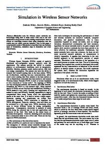
under certain fault conditions. This problem occurs due to the cycling or non-convergence of version numbers in the network. One of the properties of the reconfiguration protocol presented in Figure 1 is that starting from a good state, i.e. one in which all nodes have the same version number v, executing the protocol with a new version update v 0 such that v 0 > v will result in all nodes eventually acquiring the new version v 0 . However, an important question now arises: how does this protocol behave when started from, or somehow driven into a bad state, i.e. one in which not all nodes have the same version number. In particular, we focus on the problem of stabilizing from a global state in which all 3 version numbers exist simultaneously in the network. Figure 2 illustrates this problem in a 4-node network which has initial state as shown in (a). The ∗ symbol next to a node indicates that it will transmit next in the given interval and the edges connecting the nodes indicate wireless connectivity. As shown in the figure, after nodes 0, 1, 2 and 3 transmit in that order (Figure 2(b)-(e)), the network reaches a state in which all 3 version numbers still exist in the network. In fact, if this same sequence of broadcasts takes place in each interval, the version numbers will never converge. It can be argued that due to the random choice of the transmission instant in an interval 7

Figure 2. Cycling of version numbers during reconfiguration

for each node in action A1 of the protocol presented earlier, it is very unlikely that such a worst-case sequence can be obtained forever, and that the version numbers will eventually stabilize. However, the same argument may not hold for a much larger network in which nodes have arbitrary numbers to begin with, and in fact the version numbers may indeed keep cycling in the network forever. In general, such a scenario may occur if there exist at least 3 distinct version numbers in the network such that no one version is newer than all of the others. We call such sets of version numbers as inconsistent. Definition. A set S of distinct version numbers is defined to be inconsistent if no element of S is newer than all other elements of S. Formally, S is inconsistent ≡ (@x : x ∈ S : (∀y : y ∈ S ∧ x 6= y : x > y)) Again, recall that the > operator follows the version update rules listed earlier.

3.1 Causes of Non-stabilization In this subsection, we present some of the reasons due to which a reconfiguration protocol may enter a globally inconsistent state in which version numbers cycle through the network and may never stabilize. 1. Operator errors. Reconfiguration protocols are often designed under the assumption that only one operator or node initiates configuration updates. However, this is not always the case in practice. Large scale networks are often administered by several operators who manage different regions of the network at the same time. A common scenario in such networks is one where conflicting updates are initiated by multiple network operators. Alternatively, the same human operator may also mistakenly initiate multiple updates in an unsafe manner. As illustrated by the 8

ExScal experience in Section 1, an operator could also initialize the network in an arbitrary manner, leading to non-stabilization. 2. Transient corruption. One of the main challenges in wireless sensor networks is the severely constrained nature of node and network resources. Sensor nodes have limited processing capability, memory and battery power - all of which serve as potential sources of data corruption. Configuration updates, which are communicated as messages over the wireless channel, may be subject to corruption either due to undetected packet corruptions due to collisions or accidental buffer overwrites within the send/receive messaging stack in a node. Often, nodes store critical information such as version numbers and configuration updates in non-volatile memory such as flash to survive crashes and reboots. However, flash read/write operations may fail or return garbage values when operated under insufficient battery power. These and other such factors could result in the transient corruption of data within one or more nodes in the network, thereby producing globally inconsistent configuration sets. 3. Network dynamics. Wireless sensor networks are often deployed in harsh physical environments in which they may be subject to loss of radio connectivity and network partitioning effects. Often, subsets of wireless nodes enter a low-power sleep state for power management. Thus, under changing connectivity conditions, a sleeping node may not receive a wake-up message and may therefore miss subsequent configuration updates. Another possible scenario may occur in solar-powered networks wherein some nodes only intermittently join the network because they are deployed in sunlightdenied areas. Mobility also introduces a new challenge where nodes from a different region of the network or perhaps from another network join the network. Under all of the above conditions, the network could be left in a state where different nodes or regions of nodes in the network have different configurations, forming a globally inconsistent set.

3.2 Self-stabilization and Related Work In his seminal paper [12], Dijkstra defined a self-stabilizing protocol as one which starting from an arbitrary state, converges to a legitimate state in finite time. In [13], Katz and Perry describe a reset scheme based on a global snapshot by a central leader to achieve self-stabilization. In [14], Arora and Gouda describe a distributed reset protocol where nodes can locally initiate reset requests which are processed along a self-stabilizing spanning tree structure. In [15], Awerbuch et al. present a generalized 9

reset protocol for arbitrary graphs which uses local checking and correction to achieve self-stabilization. In [16], Awerbuch et al. extend this idea to deal with problems that can be locally checked but require global correction to achieve self-stabilization. Our work, though closely related, differs from those described above in two key aspects. First, we assume a wireless network model where we do not assume unique identifiers for nodes and neighbor links in the connectivity graph. The second difference is that in our problem, we cannot achieve selfstabilization without the involvement of an external user - the Human-In-The-Loop. Proposition 1. There does not exist a self-stabilizing reconfiguration protocol with bounded version numbers. The ideal invariant (or legitimate state) for a reconfiguration protocol can be stated as: Every node in the network has the most recent configuration. To be self-stabilizing, a reconfiguration protocol should converge to this invariant state on its own. However, in the presence of an inconsistent set, it is not possible for any node or group of nodes in the network to decide which version number is most recent due to their bounded size and rollover properties. Further, there may even be multiple configurations that share the same version number due to rollover. We therefore contend that a reconfiguration system with bounded version numbers cannot self-stabilize to the ideal invariant stated above. We therefore break down the stabilization process into two phases. In the first phase, we require the reconfiguration protocol to guarantee convergence to the following weaker invariant: Every node in the network has the same configuration. We leave the choice of deciding which configuration is the most recent one to the Human-In-The-Loop and present an external reset mechanism to achieve convergence to the ideal invariant. Despite not being fully self-stabilizing, a reconfiguration protocol that guarantees the weaker invariant presented above is quite useful in practice. Recall from Section 2.2 that reconfiguration involves not only identifying which configuration is the latest but also actually obtaining that configuration from neighboring nodes. An epidemic reprogramming protocol such as Deluge, for instance, keeps trying to download the entire program from neighbors that advertise a newer version. Thus, as long as the advertised version numbers do not stabilize, nodes will continue to expend valuable resources such as processing, radio and battery thereby resulting in degraded performance and reduced lifetime of the network. Even if this cycling problem is detected by a network operator, there is no version number 10

that the operator can download to break the cycle. However, if we guarantee stabilization to the weaker invariant, then once the protocol stabilizes to a single version, the operator can inject a higher version to update all the nodes.

4

A Stabilizing Reconfiguration Protocol In this section, we present a stabilizing solution to the reconfiguration problem discussed above. Our

solution uses local detectors and correctors to guarantee convergence to the weaker invariant without imposing any additional communication or coordination overhead. We also present an external reset mechanism initiated by the Human-In-The-Loop to achieve strong convergence.

4.1 Local Detection and Correction We first prove that the existence of a stable inconsistent set in the network can be detected locally in a bounded time. By stable, we mean an inconsistent set that does not converge before it can be detected. For sets that converge before they can be detected using our algorithm, stabilization is trivially achieved. We also prove consistency of our detectors by showing that local detection at a node implies the existence of an inconsistent set within a bounded computational history. Our detector thus does not generate any false assertions. Recall that for our canonical 3-version reconfiguration protocol, the only inconsistent set possible is {0,1,2}, each node broadcasts its version data at least once every T seconds and that n is the number of nodes and D is the diameter of the network. Theorem 1 (Completeness of local detection). For every computation starting from a state where an inconsistent version set exists in the network, and in which this inconsistency persists during the entire computation, there exists at least one node with an inconsistent set of versions in its local computation history within an interval D×T. Proof.

We first show that at least one node detects the inconsistency locally. Assume for contradiction

that this does not hold. This implies that each node in our 3-version system can assume at most 2 distinct versions in the given computation implying that its version number can change at most once. To achieve the contradiction we show that the total number of version changes in the network is a monotonically increasing function. Since an inconsistent set exists in the network, there must exist at

11

least one neighbor pair with different version numbers. It therefore follows from the protocol actions that in the next interval, at least one of these nodes must change their version number. Since the inconsistent set persists, the number of version changes exceeds n at some point implying that at least one node undergoes two version changes, thereby contradicting our assumption. We now prove that the version history of at least one node contains an inconsistent set within an interval D×T. Since inconsistency persists in the network, there must be at least two nodes with different version transitions enabled in the initial state. This is because if all nodes have no transitions or the same transitions enabled, it implies that the network has converged or will converge in the next interval. Without loss of generality, consider two nodes n1 and n2 that undergo transitions 0 → 1 and 1 → 2 respectively. Consider the shortest path between n1 and n2 and consider the immediate neighbors of n1 and n2 along this path (n01 and n02 respectively). In the next interval, n1 and n2 will either be dominated by their neighbors, dominate them or discover them to be the same. If either of n1 or n2 is dominated in the next interval, we immediately have the witness that locally detects the inconsistency. If n1 or n2 dominate their neighbors then we now have the same transitions occurring at nodes n01 and/or n02 and we can carry out the same proof for these new node pairs which are at least one hop closer to each other than the original pair. Finally, we have the case where n1 and n2 are the same as their neighbors. However, since n1 and n2 had different versions to begin with, this symmetry will be broken at some point along the path. Also, since the path between n1 and n2 can have length at most D, this symmetry-breaking will take place in D×T time which means that at least one node along this path will undergo more than one transition in a window of time D×T, leading to an inconsistent set in its local history. Theorem 2 (Consistency of local detection). In any computation with correct protocol invocation, if the local history for the last D×T time at any node contains an inconsistent set, there must exist a global state with an inconsistent set within a finite history of 2D×T in this computation. Proof.

Consider that a node whose local history at time t contains an inconsistent version set in the last

D×T time. This implies that this node assumed all 3 versions at some point in the interval [t-D×T .. t]. Without loss of generality, assume that the version observed by the node at time t is version 2. This scenario is depicted in Figure 3. From the rate assumption in Section 2.3, we know that there can be at most one reconfiguration invocation in the interval [t-D×T .. t]. If there was no invocation in this interval, no new versions could

12

Figure 3. Consistency of local detection

be added to the network after time t-D×T. Thus, if this node assumed versions 0,1 and 2 in this interval, they must all have been present in the network at time T-D×T, thereby proving the theorem. Now consider that there was one invocation in this interval. Again, without loss of generality, assume that this invocation was for version 2 as shown in the figure. This now implies that at time t-D×T, versions 0 and 1 must have been present in the network to be assumed by the node later. Now consider the time interval [t-2D×T .. t-D×T]. According to our rate assumption, there could not have been any invocations after time t’-2D×T as shown in the figure, hence there was no invocation and now new versions added during this interval. This now implies that versions 0 and 1 must have been present at time t-2D×T. However, if these were the only 2 versions present in the network at time t-2D×T, we know that they must have converged before time t-D×T. This is a contradiction. Having proven the completeness and consistency of local detection, we now present the following algorithm that performs local detection and correction. We augment the original set of version numbers with a special version number, φ, which indicates a special reset state and the update rules with the condition ∀i : i ∈ {0, 1, 2} : φ > i. Also, we update A02 from the original protocol with a set of special actions for local detection and correction. This modified action DCA02 of the original protocol shown in Figure 4 guarantees stabilization to the weaker invariant described in Section 3. Again, it should be noted that the {>, vnum) curr time := get Local T ime(); hist[] := get V ersion History(log , curr time − D×T , curr time); if is inconsistent(hist[]) vnum := φ; clear log(); else vnum := v; log := log ∪ (v , curr time); fi elseif (v < vnum) broadcast m(vnum) fi

Figure 4. Stabilizing reconfiguration using local detection/correction

this node will now periodically broadcast version φ and since φ dominates all other versions, every node in the network will switch to a null configuration with version φ within time D×T. Since we know, from Theorem 1, that an inconsistent set either converges or is detected by at least one node within D×T time, we can prove the following theorem for this stabilizing action. Theorem 3 (Local Stabilization). Starting from an arbitrary state, every execution of the locally stabilizing reconfiguration protocol stabilizes to a state where all nodes have the same value within time 2D×T.

4.2 Correction using Human-In-The-Loop The protocol actions described in the previous subsection guarantee local stabilization to the weak invariant that all nodes eventually have the same version number. Since the version φ dominates all other versions, this condition is stable. An alternate approach to local stabilization could be one in which versions present in the network are monitored by collecting a global snapshot using network querying protocols such as SNMS [17]. However, experimental studies [18] have shown that global state collection in large scale networks may only be about 50% reliable. It is therefore quite likely that a single global snapshot collected by an operator may miss the inconsistency in the network. The operator would thus have to continuously query and monitor the network - an energy expensive solution. However, since our local detectors/correctors reset the version number to φ which is then propagated in the rest of the network using the reliable update protocol itself, the operator can easily learn about the inconsistency

14

by querying only its local neighborhood. Our approach thus does not require any additional messages to be sent and also eliminates the need for global querying making it energy efficient. Upon learning of the inconsistent state in the network, the Human-In-The-Loop or the operator can take steps to restore the network to the ideal invariant by re-downloading the latest configuration update in the network. Before doing this, the operator may also choose to wake up nodes that may be in low power sleep states to avoid inconsistencies that may arise in the future. Stabilizing Reset. In the state where all nodes have version φ, the operator cannot successfully download a new configuration with any version since all nodes will reject the update due to the dominance of φ over other versions. To enable the operator to restore the network to the ideal state, we modify the original interface exposed to the operator to include a special reset operation. The purpose of the reset operation is to restore the network to a consistent state from which new configurations can be downloaded. To guarantee stabilization even in the presence of multiple initiating operators, nodes use the policy of updating their version to the predetermined value 0 upon receiving a reset. Also, a reset is a one-time operation as opposed to an epidemic one and it terminates when every node forwards the reset message once. Note that a one-time forwarding of the reset message is sufficient because of our assumption of a connected network with reliable links. A simple way of relaxing this assumption is to forward each reset message k times. When the reset operation terminates, all nodes have version 0 and the operator can now restore the network by downloading the correct (most recent) configuration with version 1. During the propagation of a reset operation, a node which has received a reset message and updated its version to 0 may roll back to a different version if it hears an advertisement from a neighbor that has not yet received the reset. To guarantee stabilization, we require that after receiving the first reset message, a node ignores all advertisements for a bounded time δ. This δ time bound is a function of the time taken for the reset to propagate in the network. We can thus prove the following theorem about the reset operation. Theorem 4 (Stabilizing Reset). Starting from an arbitrary state, executing the reset operation results in a stable state where all nodes have version 0 in bounded time. The complete stabilizing reconfiguration protocol is presented in Figure 5. The local detection and correction action is denoted as DCA02 while the reset operation is represented in action RA3 .

15

Protocol Const

Var

StabilizingP eriodicBroadcast T : integer N umV er : integer D : integer δ: real vnum : integer m : message log[] : integer × real hist[] : integer curr time : real reset start time : real sent reset : boolean

Actions [kT..(k+1)T ]

hA1 i :: T imer.f ired −→ broadcast m(vnum) [] hDCA02 i :: rcv m(v) −→ curr time := get Local T ime(); if (curr time − reset start time < δ) skip; elseif (v > vnum) hist[] := get V ersion History(log , curr time − D×T , curr time); if is inconsistent(hist[]) vnum := φ; clear log(); sent reset := F ALSE; else vnum := v; log := log ∪ (v , curr time); fi elseif (v < vnum) broadcast m(vnum) fi [] hRA3 i :: rcv m(reset) −→ reset start time := get Local T ime(); vnum := 0; if (sent reset = F ALSE) sent reset := T RU E; broadcast m(reset); fi

Figure 5. The stabilizing reconfiguration protocol

5

Performance In this section, we present results from both simulations and experiments that measure the likelihood

of non-stabilization of the canonical reconfiguration protocols in reasonable time, its impact on network performance and also the effectiveness of our local detectors and correctors in achieving stabilization.

5.1 Setup We used the TOSSIM [19] simulator to simulate the two canonical protocols described in Section 2.2. By appropriately choosing link reception probabilities, we created a regular grid topology for our simulations in which each node could communicate only with its four grid-neighbors (left, right, above and 16

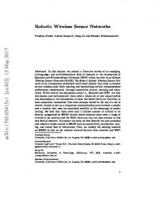
Figure 6. Performance evaluation.

below). Our experimental setup consisted of 105 XSM [20] sensor nodes deployed in a 15x7 grid in the indoor Kansei [21] testbed with 3 ft grid spacing. We used a very low power level setting of 2 to limit the transmission range and create a multi-hop network for our experiments. During the initialization phase of each simulation or experiment run, each node in the network chose its initial version number randomly from {0,1,2}. We chose the time T which is the periodicity of version advertisements in the given protocols as 15 seconds. To factor out this specific choice of the time interval, the experimental measurements and results for convergence time in this section are presented in terms of number of intervals.

5.2 Results In this subsection, we first show that the non-stabilizing version problem occurs in practice in the canonical protocols presented earlier. To say that a run is non-stabilizing, we would ideally have to let the simulation or experiment run forever. For the results presented in this section, we call a run as non-stabilizing if it did not stabilize within 50D intervals of execution time where D is the diameter of the network. We argue that this is a reasonable choice especially since we know from Theorem 1 that our local detectors and correctors will detect an inconsistency in no worse than D intervals. Hence, even if the run were to stabilize after 50D intervals, there would be a significant performance overhead. Figure 6 shows the performance of the canonical protocols and of the local stabilization strategy. The first row in the table indicates the likelihood of a run being non-stabilizing. As the data indicates, even for relatively small networks like 10×10 and 15×7, a significant number of runs in fact do not stabilize. Also, variant 2 of the broadcast protocol, in which nodes aggressively try to update their neighbors has slightly better convergence properties than variant 1, although this difference is less pronounced for the larger networks. The performance impact of non-stabilization can be seen from row 2 which shows the average number

17

of messages transmitted by a node in the network per broadcast interval. As expected, variant 1 transmits at the fixed rate of one message per interval. However, the aggressive nature of variant 2 implies that for non-stabilizing runs, it consumes significantly more resources, thereby depleting the network at a much faster rate. The third row in the table lists the average number of intervals required for convergence in runs that stabilize on their own (for non-stabilizing runs, this number is infinite), while the fourth row lists the worst case time for local stabilization using our detection and correction actions. As seen from the data, local stabilization results in faster convergence even for those runs that stabilize on their own. Recall that a reconfiguration operation also involves a data download phase operating concurrently with version update. Hence, the faster the network converges, the lesser is the amount of bandwidth and energy consumed while trying to download data. Our simulation and experimental results thus demonstrate that non-stabilization is indeed a problem that occurs in practice in existing reconfiguration protocols. Our results also validate the efficiency of the local detection and correction algorithm presented in this paper.

6

Conclusions and Future Work In this paper, we demonstrated, both theoretically and through simulations and experimental studies,

that due to different types of faults such as operator errors, data corruption, etc., there is a non-trivial probability that existing protocols for reconfiguration of wireless sensor networks may not stabilize. We presented, both qualitatively and quantitatively, the adverse impact of this non-stabilization on the quality and lifetime of the network. Our findings were validated in practice during the large scale ExScal experiments when we had to expend significant manual resources to overcome this problem. We also presented a stabilizing reconfiguration protocol that solves this problem. Our solution uses a novel mix of both autonomous and Human-In-The-Loop stabilization by locally detecting and correcting version inconsistencies, thereby allowing the human operator to easily restore the network back to the desired configuration. Our solution can be easily incorporated into existing reconfiguration protocols to make them stabilizing or can also be composed with them in the form of wrappers or interceptors to achieve stabilization. Achieving the right balance between those stabilization tasks locally performed at a node and those left to the Human-In-The-Loop is of particular interest to us. Specifically, we intend to look at problems

18

in the areas of fault monitoring and diagnostics where parts of the system run autonomously and part are managed explicitly by a human operator. We hope that this will bring us one step closer to closing the loop and creating a fully autonomous management system for wireless sensor networks.

References [1] Philip Levis and David Culler. Mat: a tiny virtual machine for sensor networks. In ASPLOS-X: Proceedings of the 10th international conference on Architectural support for programming languages and operating systems, pages 85–95, 2002. [2] C. Han, R. Kumar, R. Shea, E. Kohler, and M. Srivastava. A dynamic operating system for sensor nodes. In MobiSys ’05: Proceedings of the 3rd international conference on Mobile systems, applications, and services, pages 163–176, 2005. [3] A. Dunkels, B. Gronvall, and T. Voigt. Contiki - A Lightweight and Flexible Operating System for Tiny Networked Sensors. In LCN ’04: Proceedings of the 29th Annual IEEE International Conference on Local Computer Networks (LCN’04), pages 455–462, 2004. [4] P. Levis, N. Patel, D. Culler, and S. Shenker. Trickle: A Self-Regulating Algorithm for Code Propagation and Maintenance in Wireless Sensor Networks. In NSDI: 1st Symposium on Networked Systems Design and Implementation, pages 15–28, 2004. [5] T. Stathopoulos, J. Heidemann, and D. Estrin. A remote code update mechanism for wireless sensor networks. Technical Report CENS-TR-30, UCLA, 2003. [6] J. Hui and D. Culler. The dynamic behavior of a data dissemination protocol for network programming at scale. In SenSys ’04: Proceedings of the 2nd international conference on Embedded networked sensor systems, pages 81–94, 2004. [7] A. Arora et al. ExScal: Elements of an Extreme Scale Wireless Sensor Network. In 11th IEEE International Conference on Embedded and Real-Time Computing Systems and Applications, pages 102–108, 2005. [8] J. Zhao and R. Govindan. Understanding packet delivery performance in dense wireless sensor networks. In SenSys ’03: Proceedings of the 1st international conference on Embedded networked sensor systems, pages 1–13, 2003. [9] S. Kulkarni and M. Arumugam. TDMA Service for Sensor Networks. In ICDCSW ’04: Proceedings of the 24th International Conference on Distributed Computing Systems Workshops, pages 604–609, 2004. [10] J. Polastre, J. Hill, and D. Culler. Versatile low power media access for wireless sensor networks. In SenSys ’04: Proceedings of the 2nd international conference on Embedded networked sensor systems, pages 95–107, 2004.

19

[11] H. Zhang, A. Arora, Y. Choi, and M. Gouda. Reliable bursty convergecast in wireless sensor networks. In MobiHoc ’05: Proceedings of the 6th ACM international symposium on Mobile ad hoc networking and computing, pages 266–276, 2005. [12] E. Dijkstra. Self-stabilizing systems in spite of distributed control. Communications of the ACM, 17(11):643– 644, 1974. [13] S. Katz and K. Perry. Self-stabilizing extensions for message-passing systems. In PODC ’90: Proceedings of the ninth annual ACM symposium on Principles of distributed computing, pages 91–101, 1990. [14] A. Arora and M. Gouda. Distributed Reset. IEEE Transactions on Computers, 43(9):1026–1038, 1994. [15] B. Awerbuch, B. Patt-Shamir, and G. Varghese. Self-stabilization by local checking and correction (extended abstract). In Proceedings of the 32nd annual symposium on Foundations of computer science, pages 268–277, 1991. [16] B. Awerbuch, B. Patt-Shamir, G. Varghese, and S. Dolev. Self-Stabilization by Local Checking and Global Reset (Extended Abstract). In WDAG ’94: Proceedings of the 8th International Workshop on Distributed Algorithms, pages 326–339, 1994. [17] G. Tolle and D. Culler. Design of an Application-Cooperative Management System for Wireless Sensor Networks. In Proceedings of the EWSN’04. [18] S. Bapat, V. Kulathumani, and A. Arora. Analyzing the Yield of ExScal, a Large-Scale Wireless Sensor Network Experiment. In ICNP ’05: Proceedings of the 13TH IEEE International Conference on Network Protocols (ICNP’05), pages 53–62, 2005. [19] P. Levis, N. Lee, M. Welsh, and D. Culler. TOSSIM: accurate and scalable simulation of entire tinyOS applications. In SenSys ’03: Proceedings of the 1st international conference on Embedded networked sensor systems, pages 126–137, 2003. [20] P. Dutta, M. Grimmer, A. Arora, S. Bibyk, and D. Culler. Design of a wireless sensor network platform for detecting rare, random, and ephemeral events. In IPSN, pages 497–502, 2005. [21] OSU NEST ExScal Team. Kansei: Sensor Testbed For At-Scale Experiments. http://www.cse.ohio-state. edu/kansei.

20