... in the hospitals. Each resident has a ranking over the hospitals, and conversely, each hospital ... residents in the USA [29,32] or the detailing process of the US Navy [27]), and in the recent ... frequently studied variants are the case when preference lists involve ties and may be ...... Enlisted Assignment Process. PhD thesis ...
Stable Assignment with Couples: Parameterized Complexity and Local Search? D´ aniel Marx1 and Ildik´ o Schlotter2 1
2
Tel Aviv University, Israel Budapest University of Technology and Economics, Hungary
Abstract. We study the Hospitals/Residents with Couples problem, a variant of the classical Stable Marriage problem. This is the extension of the Hospitals/Residents problem where residents are allowed to form pairs and submit joint rankings over hospitals. We use the framework of parameterized complexity, considering the number of couples as a parameter. We also apply a local search approach, and examine the possibilities for giving FPT algorithms applicable in this context. Furthermore, we also investigate the matching problem containing couples that is the simplified version of the Hospitals/Residents with Couples problem modeling the case when no preferences are given.
1
Introduction
The classical Hospitals/Residents problem (which is a generalization of the wellknown Stable Marriage problem) was introduced by Gale and Shapley [11] to model the following situation. We are given a set of hospitals, each having a number of open positions, and a set of residents applying for jobs in the hospitals. Each resident has a ranking over the hospitals, and conversely, each hospital has a ranking over the residents. Our aim is to assign as many residents to a hospital as possible, with the restrictions that the capacities of the hospitals are not exceeded and the resulting assignment is stable. Stability will be formally defined in Section 3, but essentially an assignment is unstable, if there is a hospital h and a resident r such that r is not assigned to h, but both h and r would benefit from contracting with each other instead of accepting the given assignment. The original version of the Hospitals/Residents problem is well understood: a stable assignment always exists, and every stable assignment has the same size. (The size of an assignment is the number of residents that have a job.) Moreover, the classical Gale-Shapley algorithm [11] can find a stable assignment in linear time. However, several practical applications motivate some kind of extension or modification of the problem (see e.g. the NRMP program for assigning medical residents in the USA [29, 32] or the detailing process of the US Navy [27]), and in the recent decade various versions have been investigated. Among the most ?
Supported by ERC Advanced Grant DMMCA and by the Hungarian National Research Fund OTKA 67651.
frequently studied variants are the case when preference lists involve ties and may be incomplete [20, 21], the case when the market of the agents is one-sided, called the Stable Roommates problem [14, 15], and the case when the assignment may be a many-to-many matching [30, 4, 8]. Here we study an extension of this problem, called Hospitals/Residents with Couples, where residents may form couples, and thus have joint rankings over the hospitals. This extension models a situation that arises in many real world applications [32, 31], and was first introduced by Roth [29] who also discovered that a stable assignment need not exist when couples are involved. Later, Ronn [28] proved that it is NP-hard to decide whether a stable assignment exists in such a setting. Since then, various approaches have been investigated to deal with the intractability of this problem, but most researchers examined different assumptions on the preferences of couples that guarantee some kind of tractability [17, 5, 7, 25]. For the investigation of this problem, we use the framework of parameterized complexity which has been developed by Downey and Fellows [6]. This approach deals with hard problems, where polynomial-time algorithms are unlikely to exist. To do this, we define an integer parameter k for each problem instance, and we try to find algorithms whose running time remains tractable if the parameter k is small. More precisely, we look for algorithms whose running time is of the form f (k)nc , where n is the size of the instance having parameter k, f is an arbitrary function, and c is a constant. Note that the running time may depend exponentially or worse on the parameter k, but it yields a polynomial of degree c for each fixed k. Problems admitting such an algorithm are called fixed-parameter tractable or FPT. Up to our knowledge, no version of the Hospitals/Residents problem has been studied from the parameterized point of view. When considering Hospitals/Residents with Couples, the number of couples in an instance can be a natural parameter. We prove the negative result of Theorem 8 stating that deciding the existence of a stable assignment for the Hospitals/Residents with Couples problem is not FPT, provided that W[1] 6= FPT holds (which is a standard assumption of parameterized complexity theory). Local search is a basic technique that has been widely applied in heuristics for practical optimization problems for several decades [1]. However, investigations considering the connection of local search and parameterized algorithms have only been started a few years ago, and research in this area has been gaining increasing attention lately [22]. The basic idea of local search is to find an optimal solution by an iteration in which we improve the current solution step by step through local modifications. Local search can become more efficient if we can decide whether there exists a better solution S 0 that is ` modification steps away from a given solution S. Typically, the `-neighborhood of a solution S can be explored in nO(`) time by examining all possibilities to find those parts of S that should be modified. (Here n is the input size.) However, in some cases the dependency on ` can be improved by getting ` out of the exponent of n, resulting in a running time of the form f (`)nc for some constant c, meaning that 2
Task:
Existence problem
Maximum problem |C|
Parameter:
Local search algorithm with FPT running time `
(|C|, `)
Without preferences
P (trivial)
randomized FPT (Theorem 1)
No permissive alg. (Theorem 7)
Permissive alg. (Theorem 1)
With preferences
No FPT alg. (Theorem 8)
No FPT alg. (Theorem 8)
No permissive alg. (Theorem 10)
Strict alg. (Theorem 11)
Table 1. Summary of our results (assuming W[1] 6= FPT).
the neighborhood exploration problem is FPT. This question has already been studied in connection with different optimization problems ([16, 18, 23, 9, 33]). In Theorem 11, we give an algorithm for the following problem: given a stable assignment S, find a stable assignment S 0 of greater size which can be obtained from S by modifying the assignment for at most ` residents. The presented algorithm guesses the structure of the modification needed to obtain the larger stable assignment S 0 , and applies color-coding to localize this structure step by step in the original instance, using only simple steps. The running time of this algorithm for an instance of size n involving a set C of couples is f (`, |C|)nc for some function f and constant c, so this yields an FPT algorithm with parameters ` and |C|. In contrast, if we only regard ` as a parameter, then Theorem 10 shows that no FPT algorithm exists for this problem unless W[1] = FPT. We also contribute to the framework of parameterized local search algorithms by distinguishing between “strict” algorithms that perform the local search step in some neighborhood of a solution as described above, and “permissive” algorithms whose task is the following: given some problem with an initial solution S, find any better solution, provided that a better solution exists in the local neighborhood of S. Our motivation for this distinction is that finding an improved solution in the neighborhood of a given solution may be hard, even for problems where an optimal solution is easily found. We hope that this differentiation clarifies the role of local search in such cases, helping the parameterized complexity analysis of such problems. Most of the questions examined here are also worth studying in a model that does not involve preferences. This simplification leads to a matching problem that we call Maximum Matching with Couples. Using a result by the first author concerning matroids from the parameterized view-point [24], we propose a randomized algorithm in Theorem 1 that finds a matching of maximum size, and runs in FPT time if the parameter is the number |C| of couples. Therefore, this problem becomes easier without preferences. By contrast, the local search problem still remains hard to solve (Theorem 7). For a summary of our results see Table 1. The paper is organized as follows. Section 2 covers our notation and the preliminaries, and Section 3 introduces the formal definitions of the problems 3
examined in the paper. In Section 4, we investigate the Matching with Couples problem, and we present our results on the Hospitals/Residents with Couples problem in Section 5. Finally, we give a short summary of our results in Section 6.
2
Preliminaries
� For some integer k, we use [k] = {1, 2, . . . , k}, and [k] 2 = {(i, j) | 1 ≤ i < j ≤ k}. For a graph G, V (G) denotes its vertices and E(G) its edges. A matching in G is a set M of edges such that no two edges in M share an endpoint. If x is an endpoint of some edge in M , then x is covered by M . For some x covered by M , M (x) = y if xy ∈ M . A decision problem Q over some alphabet Σ is an arbitrary subset of Σ ∗ , and an algorithm decides Q if for every x ∈ Σ ∗ , its output is ’Yes’ if and only if x ∈ Q. With each instance of an optimization problem Q we associate a set of solutions and an objective function which we want to maximize or minimize. In this paper we consider only maximization problems. Parameterized complexity. A parameterized problem is a pair (Q, κ) where Q ⊆ Σ ∗ is a decision problem over some alphabet Σ, and κ : Σ ∗ → N is a parameterization of the problem, assigning a parameter to each instance of Q. An algorithm is fixed-parameter tractable or FPT, if its running time is f (k)|I|c for some computable function f , where I is the input, k is the parameter and c is a constant. A parameterized problem is FPT, if there is an FPT algorithm that decides it. Analogously to the classical complexity theory, the theory of W[1]-hardness can be used to prove that some problem is not FPT, unless the widely believed F P T ⊂ W [1] conjecture fails. Given two parameterized problems (Q1 , κ1 ) and (Q2 , κ2 ) over the alphabet Σ, an FPT reduction from (Q1 , κ1 ) to (Q2 , κ2 ) is a function g : Σ ∗ → Σ ∗ , computable by an FPT algorithm, such that I ∈ Q1 if and only if g(I) ∈ Q2 and κ2 (g(I)) ≤ f (κ1 (I)) for some computable function f , for every I ∈ Σ ∗ . To prove W[1]-hardness results, we use that the class of W[1]-hard problems is closed under FPT reductions. The FPT reductions in this paper are from the W[1]-hard parameterized problem Clique, in which a graph G and a parameter k is given, and the task is to decide whether there is a clique of size k in G. For further details on parameterized complexity, see e.g. [6], [26], or [10]. Local search. To formalize the task of a local search algorithm, let Q be an optimization problem with an objective function T which we want to maximize. To define the concept of neighborhoods, we suppose there is some distance d(x, y) defined for each pair (x, y) of solutions for some instance I of Q. We say that x is `-close to y if d(x, y) ≤ `. The input of a local search algorithm for Q is an instance I of Q, a solution S0 for I, and an integer `. A strict local search algorithm for Q has the following task: Strict local search for Q Input: (I, S0 , `) where I is an instance of Q, S0 is a solution for I, and ` ∈ N. Task: If there exists a solution S for I such that d(S, S0 ) ≤ ` and T (S) > T (S0 ), then output such an S. 4
In contrast, a permissive local search algorithm for Q is allowed to output a solution that is not close to S0 , provided that it is better than S0 . In local search methods, such an algorithm is as useful as its strict version. Formally, its task is as follows: Permissive local search for Q Input: (I, S0 , `) where I is an instance of Q, S0 is a solution for I, and ` ∈ N. Task: If there exists a solution S for I such that d(S, S0 ) ≤ ` and T (S) > T (S0 ), then output any solution S 0 for I with T (S 0 ) > T (S). On the one hand, note that if an optimal solution can be found by some algorithm, then this yields a permissive local search algorithm for the given problem. On the other hand, finding a strict local search algorithm might be hard even if an optimal solution is easily found. An example for such a case is the Minimum Vertex Cover problem for bipartite graphs [18]. Besides, proving that no permissive local search algorithm exists for some problem is clearly more relevant than proving that no strict local search algorithm exists for it (having a certain running time). We also present results of this kind. We remark that the distinction between permissive and strict local search algorithms cannot be maintained when addressing the standard decision version of these problems. To see this, consider the following formulation of such a local search problem: given an instance I of some optimization problem Q, a solution S0 to I, and some ` ∈ N, decide whether there is a solution S for I such that d(S, S0 ) ≤ ` and T (S) > T (S0 ). Clearly, the difference between the strict and the permissive approach is no longer applicable in this definition. Consequently, instead of proving W[1]-hardness for problems considering local search algorithms, our hardness results will be formulated as statements that no (permissive) local search algorithm can run in FPT time with a certain parameterization, assuming FPT6=W[1].
3
Problem definitions
In this section we give the formal descriptions of the different models that we investigate. Model without preferences. First, we define two versions of the Hospitals/Residents problem that involve couples, but do not deal with preferences, using only a notion of acceptability instead. A couples’ market with acceptance, or cma for short, consists of a set S of singles, a set C of couples, a set H of hospitals together with a capacity f (h) for each hospital h, a set A(s) ⊆ H for each single s ∈ S representing acceptable e for each couple c ∈ C representing acceptable hospitals for s, and a set A(c) ⊆ H e = (H ∪ {�}) × (H ∪ {�}) \ {(�, �)} where � is a hospital pairs for c. Here H special symbol indicating that someone is unemployed. If f ≡ f0 for some f0 ∈ N, then we say that the cma is f0 -uniform. Each couple c is a pair (c(1), c(2)), and 5
S we call the elements of the set R = c∈C {c(1), c(2)} ∪ S residents. The couples are mutually disjoint, i.e. each resident appears in at most one couple. An assignment for a cma (S, C, H, f, A) is a function M : R → H ∪ {�} such that M (s) ∈ A(s) ∪ {�} for each s ∈ S, M (c) ∈ A(c) ∪ {(�, �)} for each c ∈ C, and the number of residents assigned to a hospital h is at most its capacity f (h). Here, M (c) denotes the pair (M (a), M (b)) for some couple c = (a, b), and the set of residents assigned to h in M is the set {r | r ∈ R, M (r) = h}, denoted by M (h). We say that an assignment M covers a resident r if M (r) 6= �, and M covers a couple c, if it covers c(1) or c(2). We define the size of M , denoted by |M |, to be the number of residents covered by M . The Maximum Matching with Couples problem is an optimization problem, where given a cma I, the set of solutions is the set of assignments for I, and the task is to find an assignment for I of maximum size. To consider the local search versions of the Maximum Matching with Couples problem, we define the distance d(M, M 0 ) of two assignments M and M 0 for some cma I as the number of residents r for which M (r) 6= M 0 (r). Using this, the task of a strict local search algorithm for Maximum Matching with Couples is the following: given a cma I together with an assignment M for I, and some integer `, find an assignment M 0 for I with d(M, M 0 ) ≤ ` that has size greater than M . The input of a permissive local search algorithm for Maximum Matching with Couples is the same, but in this case the task is to find any assignment for I having size greater than M , if such an assignment exists in the `-neighborhood of M . Model with preferences. Next, let us define some versions of the Hospitals/Residents problem, where couples are involved and preferences play an important role. A couples’ market with preference, or cmp for short, consists of the sets S, C, and H representing singles, couples, and hospitals, respectively, a capacity f (h) for each h ∈ H, and a preference list L(a) for each a ∈ S ∪ C ∪ H. The set A = S ∪ C ∪ H is called the set of agents. The preference lists can be incomplete, but cannot involve ties, so if s ∈ S then L(s) is a strictly ordered set of hospitals, e and if h ∈ H then L(h) if c ∈ C then L(c) is a strictly ordered subset of H, e is a strictly ordered set of residents. Here, H and the symbol � are defined the same way as for the case without preferences, and we also adopt the notion of f0 -uniformity. The set of elements appearing in the list L(a) is AL (a), and we say that x is acceptable for a if x ∈ AL (a). Clearly, we may assume that acceptance is mutual, so h ∈ AL (s) holds if and only if s ∈ AL (h) for each s ∈ S and h ∈ H, and (h1 , h2 ) ∈ AL (c) implies c(i) ∈ AL (hi ) or hi = � for both i ∈ {1, 2}, for each c ∈ C. For some x ∈ AL (a), the rank of x w.r.t. a, denoted by ρ(a, x), is r ∈ N if x is the r-th element in L(a). If x ∈ / AL (a), then we let ρ(a, x) = ∞ for all meaningful x. Let I = (S, C, H, f, L) be a cmp. An assignment for I is an assignment for the underlying cma (S, C, H, f, AL ). We say that x is beneficial for the agent a with respect to an assignment M if x ∈ AL (a) and one of the following cases holds: (1) a ∈ S ∪ C and either a is not covered by M or ρ(a, x) < ρ(a, M (a)), 6
(2) a ∈ H and either |M (a)| < f (a) or there exists a resident r 0 ∈ M (h) such that ρ(a, x) < ρ(a, r 0 ). A blocking pair for M can be of three types: – it is either a pair formed by a single s and a hospital h such that both s and h are beneficial for each other w.r.t. M , – or a pair formed by a couple c and a pair (h1 , h2 ) with h1 6= h2 such that (h1 , h2 ) is beneficial for c w.r.t. M , and for both i ∈ {1, 2} it holds that if hi 6= � then either c(i) is beneficial for hi w.r.t. M or c(i) ∈ M (hi ), – or a pair formed by a couple c and a hospital h such that (h, h) is beneficial for c w.r.t. M , and the couple c is beneficial for h. If h prefers c(1) to c(2), this latter means that either |M (h)| ≤ f (h) − 2, or |M (h)| ≤ f (h) − 1 and ρ(h, c(1)) < ρ(h, r) for some r ∈ M (h), or ρ(h, c(1)) < ρ(h, r1 ) and ρ(h, c(2)) < ρ(h, r2 ) for some r1 6= r2 in M (h). 3
An assignment M for I is stable if there is no blocking pair for M . The input of the Hospitals/Residents with Couples problem is a cmp I, and the task is to determine a stable assignment for I, if such an assignment exists. We denote by Maximum Hospitals/Residents with Couples the optimization problem where the task is to determine a stable assignment of maximum size for a given cmp. Another variant of this optimization problem which we will address is the Increase Hospitals/Residents with Couples problem. Here, the input is a cmp I and a stable assignment M0 for I, and the task is to find a stable assignment with size at least |M0 |+1.
4
Matching without preferences
In this section we investigate the parameterized complexity of the Maximum Matching with Couples problem. In Subsection 4.1 we present a randomized FPT algorithm for it, where the parameter is the number of couples. Then we turn our attention to an application of this algorithm in the context of scheduling problems in Subsection 4.2. We also examine the possibility of finding a local search algorithm for the Maximum Matching with Couples problem in Subsection 4.3. 4.1
Fixed-parameter tractability
Let us examine the complexity of the Maximum Matching with Couples problem. Clearly, if there are no couples in a given instance, then the problem is equivalent to finding a maximum matching in a bipartite graph, and can be solved by standard techniques. If couples are involved, the problem becomes hard. More precisely, the decision version of this problem is NP-complete [13, 3], even in the special case where each hospital has a capacity of 2, and the acceptable hospital pairs for a couple are always of the form (h, h) for some h ∈ H. However, if the number of couples is small, which is a reasonable assumption in many practical applications, Maximum Matching with Couples becomes tractable, as shown by Theorem 1. 3
We thank David Manlove for pointing out this case.
7
Theorem 1. Maximum Matching with Couples can be solved in randomized FPT time with parameter |C|. We will use the following lemma to solve a special case of the Maximum Matching with Couples problem. Lemma 2. There exists an algorithm running in randomized FPT time with parameter |C| that, given an instance of the 1-uniform Maximum Matching with Couples problem and some integer n, finds an assignment covering at least n singles and also each resident that is a member of some couple, if such an assignment exists. To prove Lemma 2, we need some results from [24] concerning matroids. Although we only use basic concepts from matroid theory, here we give a brief outline of the main definitions used. For some set U and collection I ⊆ 2U , the pair (U, I) is a matroid if the following hold: (1) ∅ ∈ I, (2) if X ∈ I and X 0 ⊆ X then X 0 ∈ I, and (3) if X, Y ∈ I and |X| < |Y | then X ∪ {y} ∈ I for some y ∈ Y \ X. The elements of I are called independent sets. A matrix A over a field F is a linear representation of a matroid ({ui | i ∈ [n]}, I), if for any set J of indices in [n], the set of columns in A corresponding to the indices J are independent over F if and only if {uj | j ∈ J} ∈ I. A matroid is linear if it admits a linear representation. A maximal independent set of a matroid is called a basis of the matroid. The dual of a matroid (U, I) with basis set B is the matroid with ground set U whose basis set is {U \ B | B ∈ B}. The k-truncation of (U, I) is the matroid (U, I 0 ) where I ∈ I 0 if and only if I ∈ I and |I| ≤ k. Given a bipartite graph G(A, B; E), its transversal matroid has ground set A, and X is defined to be independent if there is a matching in G covering X. Theorem 3 ([24]). Let M(U, I) be a linear matroid where the ground set U is partitioned into blocks of size b. Given a linear representation A of M, it can be determined in f (k, b) · ||A||O(1) randomized time whether there is an independent set that is the union of k blocks. (||A|| denotes the length of A in the input.) The following generalization of Theorem 3 will be convenient for our purposes. Corollary 4. Let M(U, I) be a linear matroid and let X = {X1 , X2 , . . . Xn } be a collection of subsets of U , each of size b. Given a linear representation A of M, it can be determined in f (k, b) · ||A||O(1) randomized time whether there is an independent set that is the union of k disjoint sets in X . Proof. First, let us make n(u) copies for each u ∈ U , where n(u) is the number of sets in X containing u, i.e. let U 0 = {ui | u ∈ U, n(u) > 0, i ∈ [n(u)]}. Let M0 (U 0 , I 0 ) be the matroid where I 0 contains those sets which can be obtained from some set I ∈ I by replacing each u ∈ I with an arbitrary element from {ui | i ∈ [n(u)]}. A representation A0 of M0 can be obtained from A by putting n(u) copies of the column representing u into A0 for each u ∈ U . For each i ∈ [n], let Xi0 ⊆ U 0 be obtained by replacing each element u in Xi with uj if Xi is the j-th 8
set in X containing u. Clearly, by letting Xi0 be a block (having size b) for each i ∈ [n], we get a partition of U 0 . The sets {Xij | j ∈ [k]} satisfy the requirements (being disjoint and having an independent union in M) if and only if the sets {Xi0j | j ∈ [k]} are k blocks whose union is independent in M0 , and thus the algorithm of Theorem 3 provides the solution. t u Lemma 5 ([24]). (1) Given a representation A over a field F of a matroid M, a representation of the dual matroid M∗ over F can be found in polynomial time. (2) Given a representation A over N of a matroid M and an integer k, a representation of the k-truncation of Mk can be found in randomized polynomial time. (3) Given a bipartite graph G(A, B; E), a representation of its transversal matroid over N can be constructed in randomized polynomial time. Now, we are ready to prove Lemma 2. Proof (of Lemma 2). Let (S, C, H, f, A) be the given cma with f ≡ 1 for which we have to find an assignment covering at least n singles and each resident that is a member of some couple in C. Clearly, we can assume A(c) ⊆ H × H. Let G(H, S; E) be the bipartite graph where a single s ∈ S is connected with a hospital h ∈ H if and only if h ∈ A(s). We can assume w.l.o.g. that G has a matching of size at least n as otherwise no solution may exist, and this case can be detected easily in polynomial time. We define M(H, I) to be the matroid where a set X ⊆ H is independent if and only if there is a matching in G that covers at least n singles but covers no hospitals from X. Observe that M is exactly the dual of the n-truncation of the transversal matroid of G, and thus it is indeed a matroid. By Lemma 5, we can find a linear representation A of M in randomized polynomial time. We define the matroid M0 (U, I 0 ) with ground set U = H ∪ C such that X ⊆ U is independent in M0 if X ∩ H is independent in M. A representation of M0 can be obtained by appending a unit matrix of size k × k to A in the intersection of k newly introduced rows and columns, each containing only zeros in the remaining entries. Let X be the collection of the sets that are of the form {c, h1 , h2 } where c ∈ C and (h1 , h2 ) ∈ A(c). Observe that if X1 , X2 , . . . , Xk are k disjoint sets in X whose union is independent in M0 , then we can construct an assignment covering each resident that is a member of some couple and at least n additional singles as follows. For each {c, h1 , h2 } ∈ {X1 , . . . , Xk } we choose M (c) from {(h1 , h2 ), (h2 , h1 )} ∩ A(c) arbitrarily. The disjointness of the sets X1 , . . . , Xk guarantees that this way we S assign exactly one resident to each hospital in X = i∈[k] Xi ∩ H. Now, let N be a matching in G that covers at least n singles, but no hospitals from X. Such a matching exists, as X is independent in M. Thus, letting M (s) be N (s) if s is covered by N and � otherwise for each s ∈ S yields that M is an assignment with the desired properties. Conversely, if M is an assignment covering each member of the couples and n additional singles, then the sets {c, h1 , h2 } for 9
each c ∈ C and M (c) = (h1 , h2 ) form a collection of k disjoint sets in X whose union is independent in M0 . By Corollary 4, such a collection can be found in randomized FPT time when k is the parameter, yielding a solution if exists. t u Using Lemma 2, we can prove Theorem 1. Proof. Let I = (S, C, H, f, A) be the given cma in the Maximum Matching with Couples problem. We give an algorithm that decides whether there is an assignment covering t residents in this instance. First, we reduce the general problem to the 1-uniform case by “cloning” the hospitals. To this end, substitute each h ∈ H with newly introduced hospitals h1 , . . . , hf (h) ; the set of acceptable residents will be A(h) for each of these hospitals. Now, for each single s and for each hospital h acceptable for s, replace h with the elements h1 , . . . , hf (h) in the set of acceptable hospitals for s. Also, for each couple c and for each entry (ha , hb ) in A(c), replace the entry (ha , hb ) in the set of of acceptable hospital pairs for c with the elements in {(hia , hjb ) | i ∈ [f (ha )], j ∈ [f (hb )]}. (The cases where ha = � or hb = � can be handled similarly.) It is easy to see that an assignment for I covering a certain set of residents can be transformed into an assignment for the modified instance covering exactly the same residents, and vice versa. Note that this modification increases the input 2 length of the instance by at most a factor of fmax , where fmax is the maximum capacity of some hospital in H. Since we can assume fmax ≤ |S| + 2|C| without losing generality, this means that the input increases only by a polynomial factor. Next, we show how to solve the 1-uniform Maximum Matching with Couples problem using the algorithm of Lemma 2. For each couple c ∈ C, we branch into three cases, according to the cases where want to cover 0, 1, or 2 of the residents of the couple c. In the branch where we do not want to cover any member of c, we simply delete c from the market. In the branch where we only want to cover one member of the couple c, we can replace c with a new single sc that finds exactly those hospitals h acceptable for which either (�, h) or (h, �) was acceptable for c. (We also have to replace the members of c with sc in the acceptance lists of the hospitals.) After branching for each couple in C, we look for an assignment that covers each resident in the remaining set C 0 of couples, and also t − 2|C 0 | additional singles. This task can be accomplished by using the algorithm of Lemma 2. Notice that the branchings only increase the running time by a factor of 3|C| . Clearly, such an assignment yields an assignment of size t in the original instance I. Conversely, if there is an assignment of size t in I, then at least one branch will lead to such an assignment. t u We remark that the main obstacle to derandomize the algorithm of Theorem 1 is the fact that the proof of Theorem 3 makes use of the Zippel-Schwartz Lemma in some issues connected to matroid representations, and hence is inherently randomized (see also [24]). 10
4.2
An application in scheduling
Lemma 2 can be generalized in a straightforward way to the case when there are groups having some fixed size p ∈ N instead of couples of size 2 in the given market. Then, in the proof of Lemma 2 we have to use blocks of size p+1 instead of size 3, and hence we need to apply Corollary 4 with setting b = p + 1. The running time of this more general version of the algorithm is randomized FPT, if we regard both the number of groups and p as parameters. This has a useful consequence in connection to the following scheduling problem. We are given a set M of parallel machines and a set J of independent jobs. With each job j ∈ J we associate a processing time pj and a processing set Mj ⊆ M of machines that can process j. The task is to find a scheduling where each job j is (entirely) processed by a machine in Mj . Formally, a scheduling in this setting is an assignment µ : J → M mapping each job j ∈ J to some machine inPits processing set Mj . The makespan of a scheduling µ is the value maxm∈M µ(j)=m pj , which describes the latest completion time when some machine in M finishes all the jobs assigned to it. We consider the following problem in this context: given the set of jobs with their processing times and processing sets, find a scheduling that minimizes the makespan. In the standard three-field notation of the area of scheduling algorithms, this problem is abbreviated as P |Mj |Cmax . Similar scheduling problems have been widely studied by researchers, see the recent survey of Leung and Li [19]. Due to the computational hardness of these problems, most of the work in this area focuses on either approximation or exponential-time algorithms. Also, researchers have extensively studied special cases which are more likely to be tractable, such as scheduling with unit length jobs, or cases where the job processing restrictions exhibit some specific structure. Here we complement this line of research by providing a randomized fixedparameter tractable algorithm for the special case of the P |Mj |Cmax problem where k jobs have processing time p ∈ N and all other jobs have processing time 1, and we regard k as a parameter. This problem was proved to be NPcomplete even if p = 2 (see [13, 3]), so investigating the parameterized complexity of this problem might be of practical importance. Theorem 6. There is a randomized FPT algorithm for the special case of the P |Mj |Cmax problem where k jobs have processing time p ∈ N and all other jobs have processing time 1, and we regard k and p as the parameter. Proof. Let us be given some instance I of the P |Mj |Cmax problem where k jobs have processing time p ∈ N and all other jobs have processing time 1. Let J and M denote the set of jobs and machines, and let pj and Mj denote the processing time and the processing set for some job j ∈ J, respectively. To construct a minimum makespan scheduling, we will use the generalized version of the algorithm presented in Lemma 2, dealing with case when there are groups of some fixed size p instead of couples having size 2 in the market. This algorithm runs in randomized FPT time, if both k and p are parameters. 11
We provide an algorithm that for any T ∈ N can construct a scheduling for the given instance I with makespan at most T , if such a scheduling exists. By applying a binary search on the value of T we can extend this to finding a minimum makespan scheduling. For a given value T ∈ N, we construct a 1uniform cma as follows. Let z = bT /pc. For each machine m ∈ M we define T hospitals h1m , h2m , . . . , hTm (each with capacity 1). For each job j with processing time 1, we add a corresponding single resident sj that finds exactly the hospitals in {him | m ∈ Mj , i ∈ [T ]} acceptable. For each job j with processing time p, we add a corresponding group gj consisting of p newly introduced residents, and we (i−1)p+1 (i−1)p+2 let the acceptable p-tuple of hospitals for gj be {(hm , hm , . . . , hip m) | m ∈ Mj , i ∈ [z]}. We apply the generalized version of the algorithm of Lemma 2 to find an assignment covering each resident in this instance. Note that the number of groups is k (the number of jobs with processing time p) and the number of singles is |J| − k (the number of remaining jobs). It is also easy to see that the construction time is polynomial in T and the original input length, observe that T ≤ p|J| can also be assumed. Thus, the presented algorithm runs in randomized FPT time with parameters k and p. It remains to show the correctness of the algorithm. First we prove that any assignment covering each resident can be used to construct a scheduling µ for I with makespan at most T as follows. If some single sj is assigned to some hospital in him , then we let µ(j) = m; note that µ(j) ∈ Mj holds. Similarly, for each (i−1)p+1 group gj assigned to a p-tuple of hospitals (hm , . . . , hip m ) for some m ∈ Mj and i ∈ [z], we let µ(j) = m. Clearly, this is a scheduling for I with makespan at most T . For the other direction, suppose that µ is a scheduling with makespan T . Let Jm be the set of jobs assigned to some machine m, and suppose that Jm contains the jobs jx1 , . . . , jxa with processing time p, and the jobs jy1 , . . . , jyb with processing time 1. In this case, we assign each group gxi to the p-tuple of hospitals (i−1)p+1 pa+i (hm , . . . , hip . It is easy m ), and we assign each single syi to the hospital hm to verify that this way we indeed obtain an assignment in the constructed cma covering each resident. t u 4.3
Local search
Here, we investigate the applicability of the local search approach to handle the intractability of the Maximum Matching with Couples problem. Theorem 7. There is no permissive local search algorithm for the 2-uniform Maximum Matching with Couples that runs in FPT time with parameter ` denoting the radius of the explored neighborhood, unless W[1] = FPT. Proof. Let G be the input graph for the Clique problem and k be the parameter given. We denote the vertices of G by v1 , v2 , . . . , vn . We claim that if there is a permissive local search algorithm A for Maximum Matching with Couples running in FPT time with parameter `, then we can use A to solve Clique in FPT time. To prove this, we construct an input Λ = (I, M0 , `) of A with the 12
following properties: every assignment for I with size at least |M0 | + 1 is `-close to M0 , and there is such an assignment for I if and only if G has a clique of size k. Thus, G has a clique of size k if and only if A outputs an assignment for I with size at least |M0 | + 1. To construct Λ, we first define the cma I together with S the assignment M0 for it. Let the set H of hospitals be the union of D = B ∪ {H i,j | i, j ∈ [k]}, S 0i,j 0 0 D = B ∪ {H | i, j ∈ [k]} and F = {fi | i ∈ [k]}, where B = {bi | i ∈ i,j [2k − 1]}, H i,i = {hi,i = {hi,j x,y | vx vy ∈ E(G)} for j,j | j ∈ [n]} for each i ∈ [k], H each i 6= j, {i, j} ⊆ [k], and for each hospital h in B (H i,j , respectively) we also define a hospital h0 to be in B 0 (H 0i,j , respectively). For brevity, we will use the i,j i,j i,j i,j i,j notation Hh,• = {h | ∃y : h = hi,j h,y ∈ H } and H•,h = {h | ∃x : h = hx,h ∈ H }. The capacity of each hospital is 2. For each hospital h ∈ D we define a couple denoted by c(h), and for each h0 ∈ D0 we define two singles s1 (h0 ) and s2 (h0 ). Let C = {c(h) | h ∈ D} and let S = {s0 } ∪ {si (h0 ) | h0 ∈ D0 , i ∈ {1, 2}}. Before defining A(p) for each p ∈ S ∪ C, we define the assignment M0 for I, as this will not cause any confusion. Let M0 (s0 ) = �, and let M0 (p) = h where either h ∈ D and p is a member of the couple c(h), or h ∈ D 0 and p ∈ {s1 (h), s2 (h)}. Now, for each p ∈ S ∪ C, we define the set of acceptable hospitals or pairs of hospitals A(p) to be the union of {M0 (p)} and the set A0 (p) of hospitals, defined below, that can be assigned to p besides M0 (p). We define A0 (p) for each p ∈ S ∪ C as follows. A0 (c(h)) = {(h0 , h0 )} for each h ∈ D A0 (s0 ) = {b1 } A0 (s1 (b0i )) = H 1,i for each i ∈ [k] A0 (s2 (b0i )) = {bi+1 } for each i ∈ [k] A0 (s1 (b0k+i )) = H i,1 for each i ∈ [k − 1] A0 (s2 (b0k+i )) = {bk+i+1 } for each i ∈ [k − 2] A0 (s2 (b02k−1 )) = H k,1 i,j+1 A0 (s1 (h0i,j for each i ∈ [k], j ∈ [k − 1] and every possible x and y x,y )) = Hx,• 0 0i,k A (s1 (hx,y )) = {fi } for each i ∈ [k] and every possible x and y i+1,j A0 (s2 (h0i,j for each i ∈ [k − 1], j ∈ [k] and every possible x and y x,y )) = H•,y 0 0k,i A (s2 (hx,y )) = {fi } for each i ∈ [k] and every possible x and y This completes the definition of the cma I = (S, C, H, f, A). Observe that M0 indeed is an assignment for I. Finally, setting ` = 4k 2 + 8k − 3 finishes the definition of the instance Λ = (I, M0 , `). Figure 1 shows an illustration. First, suppose that M is an assignment for I such that |M | > |M0 |. We do not require M to be (4k 2 +8k −3)-close to M0 , but we will actually prove that this is necessary. Observe that M0 covers each resident except for s0 , so M must cover all residents to satisfy |M | > |M0 |. As A(s0 ) = {b1 }, M must assign b1 to s0 . This implies M (c(b1 )) = (b01 , b01 ), and therefore we also have M (s2 (b01 )) = b2 , implying M (c(b2 )) = (b02 , b02 ), and so on. Following this argument, it can be seen that M (c(bi )) = (b0i , b0i ) for every i ∈ [2k − 1], and M (s2 (b0i )) = bi+1 for every i ∈ [2k − 2]. 13
b1 b01
H k,1 H 0k,1
bi b0i
bk−1 b0k−1
bk b0k
bk+1 b0k+1
H 1,1 H 01,1
H 1,i H 01,i
H 1,k H 01,k
f1
bk+i b0k+i
H i,1 H 0i,1
H i,i H 0i,i
H i,k H 0i,k
fi
b2k−1 b02k−1
fk−1 H k,1 H 0k,1
H k,i H 0k,i
H k,k H 0k,k
fk
Fig. 1. A block diagram showing the hospitals in the proof of Theorem 7. For two sets H1 , H2 of hospitals, (H1 , H2 ) is an arc if A0 (s) ⊆ H2 for some s ∈ S with M0 (s) ∈ H1 .
We say that a single s enters H i,j if M (s) ∈ H i,j but M0 (s) ∈ / H i,j , and leaves 0i,j 0i,j H if M0 (s) ∈ H but M (s) ∈ / H . A couple c moves from a hospital h if M0 (c) = (h, h) 6= M (c), and we say that c moves from a set J ⊆ H of hospitals if it moves from a hospital in J. Observe that if c moves from H i,j , then two singles leave H 0i,j , one of them entering H i+1,j if i 6= k, and the other entering H i,j+1 if j 6= k. If a single s leaves H 0i,j but does not enter H i+1,j or H i,j+1 , then M (s) ∈ F must hold, and therefore there can exist at most 2k such single s. Moreover, if a set of m singles enter H i,j then at least dm/2e couples have to move from H i,j . For each i ∈ [k], exactly one single from {s1 (b01 ), s1 (b02 ), . . . , s1 (b0k )} enters H 1,i , and exactly one single from {s1 (b0k+1 ), s1 (b0k+2 ), . . . , s1 (b02k−1 ), s2 (b02k−1 )} enters H i,1 . These altogether imply that exactly one couple moves from H i,j for each i, j ∈ [k], and that if s and s0 enter H i,j then M (s) = M (s0 ) must hold. Suppose that c moves from the hospital hi,j x,y . Observe that if j < k then a i,j+1 couple must move from Hx,• , and similarly, if i < k then a couple must move i+1,j from H•,y . For each i ∈ [k], letting σh (i) be x if for some j a couple moves j,i i,j , we obtain , and σv (i) be y if for some j a couple moves from H•,y from Hx,• that σh (i) and σv (i) are well-defined. Observe that by the definition of H i,i we get σh (i) = σv (i) := σ(i), and from the definition of H i,j we get that if σ(i) = x and σ(j) = y for some i 6= j, then vx vy must be an edge in G. Thus, the set {vσ(i) | i ∈ [k]} forms a clique of size k in G. Remember that exactly one couple moves from H i,j for each i, j ∈ [k], which (considering also the size of F ) forces exactly two singles to leave H 0i,j for each i, j ∈ [k]. Taking into account the couples c(bi ) and the singles s1 (b0i ), s2 (b0i ) for each i ∈ [2k − 1] and the single s0 , we get that M is 4k 2 + 4(2k − 1) + 1 = (4k 2 + 8k − 3) = `-close to M0 . 0i,j
14
Now, suppose vσ(1) , vσ(2) , . . . , vσ(k) form a clique in G. By defining M as below, it is straightforward to verify that M is an assignment for (S, C, H, f, A) which covers every resident, and is `-close to M0 . M (c(bi )) = (b0i , b0i ) for each i ∈ [2k − 1] 0i,j 0i,j M (c(hi,j σ(i),σ(j) )) = (hσ(i),σ(j) , hσ(i),σ(j) ) for each i, j ∈ [k] M (s0 ) = b1 M (s1 (b0i )) = h1,i σ(1),σ(i) for each i ∈ [k]
M (s1 (b0k+i )) = hi,1 σ(i),σ(1) for each i ∈ [k − 1]
M (s2 (b02k−1 )) = hk,1 σ(k),σ(1) M (s2 (b0i )) = bi+1 for each i ∈ [2k − 2] i,j+1 M (s1 (h0i,j σ(i),σ(j) )) = hσ(i),σ(j+1) for each i ∈ [k], j ∈ [k − 1] i+1,j M (s2 (h0i,j σ(i),σ(j) )) = hσ(i+1),σ(j) for each i ∈ [k − 1], j ∈ [k]
M (s1 (h0i,k σ(i),σ(k) )) = fi for each i ∈ [k]
M (s2 (h0k,i σ(k),σ(i) )) = fi for each i ∈ [k] M (p) = M0 (p) for every p ∈ S ∪ C where M (p) was not defined above.
t u
Let us now remark that the proof of Theorem 7 implicitly contains an FPT reduction from Clique to the decision version of the local search problem for the 2-uniform Maximum Matching with Couples. However, as discussed in Section 2, the presented result is stronger than a W[1]-hardness proof.
5
Matching with preferences
In this section, we study the Hospitals/Residents with Couples problem in detail. If no couples are involved, then a stable assignment for a given couples’ market with preferences can always be found in linear time with the Gale-Shapley algorithm [11]. In the case when couples are present, a stable assignment may not exist, as first proved by Roth [29]. Here we also give a simple example. Let H = {h1 , h2 , h3 }, S = ∅, C = {(a, b), (c, d)} and f ≡ 1. The preference lists are defined below. It is straightforward to verify that no stable assignment exists for this cmp which will be denoted by I0 . For example, M (a) = h1 , M (b) = h2 and M (c) = M (d) = � is not stable, because (c, d) and (h1 , h3 ) form a blocking pair. L((a, b)) : (h1 , h2 ), (h2 , h3 ), (h3 , h1 ) L((c, d)) : (h1 , h3 ), (h2 , h1 ), (h3 , h2 )
L(h1 ) = L(h2 ) = L(h3 ) : c, a, b, d
Ronn proved that deciding whether a stable assignment exists for a cmp is NP-complete [28]. As the following example shows, an instance of the Hospitals/Residents with Couples problem may admit stable assignments of 15
different sizes. The example contains a single s, a couple c = (c1 , c2 ) and hospitals h1 and h2 with capacities f (h1 ) = 2 and f (h2 ) = 1. The preference lists are the following: L(s) : h2 , h1 L(h1 ) : s, c1 , c2 L(c) : (h1 , h1 ), (�, h2 ) L(h2 ) : c2 , s In this instance, assigning s to h1 and c to (�, h2 ) yields a stable assignment of size 2, whilst assigning s to h2 and c to (h1 , h1 ) results in a stable assignment of size 3. Note that Maximum Hospitals/Residents with Couples problem, where the task is to determine a stable assignment of maximum size for a given cmp, is trivially NP-hard, as it contains the Hospitals/Residents with Couples problem. The parameterized complexity of Hospitals/Residents with Couples is covered in Subsection 5.1. In Subsection 5.2, we present results concerning the applicability of local search for the Maximum Hospitals/Residents with Couples problem. 5.1
Fixed-parameter tractability
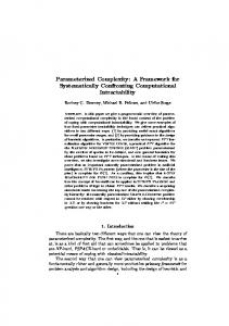
The main result of this subsection is Theorem 8, which shows the W[1]-hardness of the Hospitals/Residents with Couples problem with parameter |C|. As a consequence, the optimization problem Maximum Hospitals/Residents with Couples is also W[1]-hard with parameter |C|. However, supposing that a stable assignment has already been determined by some method, it is a valid question whether we can increase its size. Given a cmp I and a stable assignment M0 for I, the Increase Hospitals/Residents with Couples problem asks for a stable assignment with size at least |M0 |+1. If no couples are involved, then all stable assignments for the instance have the same size, so this problem is trivially polynomial-time solvable. Theorem 8 shows that Increase Hospitals/Residents with Couples is also W[1]-hard with parameter |C|. Theorem 8. (1) The decision version of Hospitals/Residents with Couples is W[1]-hard with parameter |C|, even in the 1-uniform case. (2) The decision version of Increase Hospitals/Residents with Couples is W[1]-hard with parameter |C|, even in the 1-uniform case. Before proving Theorem 8, we introduce a special construction that will be very useful in the proof. For a graph G and an integer k, we construct a cmp I G,k = (S, C, H, f, L) as follows. See Figure 2 for an illustration. Let V (G) = {vi | i ∈ [n]}, |E(G)| = m and let ν be a bijection from [m] into the set {(x, y) | vx vy ∈ E(G), x < y}. First, we construct a node gadget G i for � each i ∈ [k] and an edge gadget G i,j for each pair (i, j) ∈ [k] 2 . The node gadget G i contains hospitals H i ∪Gi ∪{f i }, singles S i ∪T i and a couple ai . Analogously, the edge gadget G i,j contains hospitals H i,j ∪ Gi,j ∪ {f i,j }, singles S i,j ∪ T i,j and a couple ai,j . Here T i = {tij | j ∈ [n − 1]} and T i,j = {ti,j e | e ∈ [m − 1]}, 16
Gi
Si 2
2 n+1 1 i 2
Hi
1 di1 1 di2
1
1 1
2
G i,j
Ti
Gi 2 1
4
1 2
3
f
f ai
n 2
1 din
1
S i,j H i,j
m+1 1 4 i,j 2
1
2
1
2
1
1
1
2
m 32
4
2
2 1
1 2
3
ai,j
1 1
Gi,j T i,j
1
2
1
32
1 1
2
Fig. 2. A node gadget and an edge gadget of I G,k . Hospitals are represented by rectangles, singles by black circles, and members of couples by double circles. A hospital h is connected to some resident r if r ∈ AL (h). The numbers on the edges represent ranks, bold edges represent M0G,k from Lemma 9, and dix is for |Qix | + 2. i i H i = {hij | j ∈ [n]} and H i,j = {hi,j e | e ∈ [m]}, and we define G , S and � k Gi,j , S i,j similarly to H i and H i,j . Observe that |C| = k + 2 . We let f ≡ 1, so I G,k is 1-uniform. The precedence lists for each agent in I G,k are defined below. The notation [X] for some set X in a preference list denotes an arbitrary ordering of the elements of X. We write Qix for the set j,i {si,j e | i < j ≤ k, ∃y : ν(e) = (x, y)} ∪ {se | 1 ≤ j < i, ∃y : ν(e) = (y, x)} and i,j i j Qe for {hx , hy } where ν(e) = (x, y). The indices in the precedence lists take all possible values if not stated otherwise, and the symbol α can be any index in [k] � or a pair of indices in [k] 2 . If α takes a value in [k] then N (α) = n, otherwise N (α) = m. (This notation will be used again later on.) α α L(gxα ) : tα if 1 < x < N (α) L(hix ) : ai (1), [Qix ], six x−1 , a (2), tx α α α i,j i,j L(g1 ) : a (2), t1 L(hi,j e ) : a (1), se α α i i i α α L(sx ) : hx , f L(gN (α) ) : tN (α)−1 , a (2), a (1) α α α i,j i,j i,j L(tx ) : gx , gx+1 L(si,j e ) : he , [Qe ], f α α α α α L(f ) : s1 , s2 , . . . , sN (α) , a (2) α α α α α α α α L(aα ) : (gN (α) , f ), (h1 , gN (α) ), (h2 , gN (α)−1 ), . . . , (hN (α) , g1 )
Lemma 9. For a graph G and k ∈ N, I G,k has a stable assignment M0G,k that covers each resident. Moreover, statements (1), (2) and (3) are equivalent: (1) There is a clique in G of size k. (2) There is a stable assignment M for I G,k with the following property, which � we will call property π: M (f i,j ) ⊆ S i,j for each (i, j) ∈ [k] 2 . (3) There is a stable assignment for I G,k with property π covering each resident. Proof. To see the first claim, we define an assignment M0 by letting M0 (aα ) = α α α α α α (gN (α) , f ), M0 (tx ) = gx , and M0 (sx ) = hx for all possible values of α and x. As each single and couple is assigned to his or their best choice, M0 is stable and covers each resident. 17
To prove (2) ⇒ (1), suppose that I G,k has a stable assignment M with � property π. Let us define σ(i, j) for each (i, j) ∈ [k] such that M (f i,j ) = 2 i,j i,j i,j i,j i,j {si,j σ(i,j) }. Since sσ(i,j) prefers hσ(i,j) to f , M (hσ(i,j) ) = {a (1)} follows from i,j i,j the stability of M . From this, we get that M (se ) = he must hold for each i,j e ∈ [m] \ {σ(i, j)} since otherwise si,j e and he would form a blocking pair. Note i,j that each single in S is assigned to a hospital in H i,j ∪ {f i,j }. As this holds for � i i i each (i, j) ∈ [k] 2 , we get that M (hx ) ⊆ S ∪{a� (1)} holds for each i ∈ [k], x ∈ [n]. [k] Let ν(σ(i, j)) = (x, y) for some (i, j) ∈ 2 . Since si,j σ(i,j) prefers the hospitals i j i,j in Qi,j , M can only be stable if both hix and hjy prefer their σ(i,j) = {hx , hy } to f
i i j j partner in M to si,j σ(i,j) . This implies M (hx ) = {a (1)} and M (hy ) = {a (1)}. i Thus, by defining σ(i) to be x if M (ai ) = (hix , gn+1−x ) for each i ∈ [k], we obtain ν(σ(i, j)) = (σ(i), σ(j)). From the definition of ν, this implies that vσ(i) � and vσ(j) are adjacent in G. As this holds for every (i, j) ∈ [k] 2 , we get that {vσ(i) | i ∈ [k]} is a clique in G. Now we prove (1) ⇒ (3). If vσ(1) , vσ(2) , . . . , vσ(k) form a clique in G, then define σ(i, j) such that σ(i, j) = ν −1 (σ(i), σ(j)). We define a stable assignment M fulfilling property π and covering every resident as follows. α M (sα σ(α) ) = f α α M (sx ) = hx if x ∈ [N (α)] \ {σ(α)} i M (aα ) = (hα σ(α) , gN (α)+1−σ(α) ) α α M (tx ) = gx if 1 ≤ x < N (α) + 1 − σ(α) α M (tα if N (α) + 1 − σ(α) ≤ x < N (α) x ) = gx+1
It is not hard to verify the stability of M by simply checking all possibilities to find a blocking pair. (We note that many of the agents are only contained in I G,k to assure that a clique in G indeed implies a stable assignment with the required properties.) As (3) ⇒ (2) is trivial, this finishes the proof. t u
Proof (of Theorem 8). Let G be an arbitrary graph and k ∈ N. We construct two 1-uniform cmps I1 and I2 , together with a stable assignment M2 for I2 such that the following three statements are equivalent: (a) G has a clique of size k, (b) I1 has a stable assignment, (c) I2 has a stable assignment of size greater than |M2 |.
� Furthermore, the construction will take FPT time, and there will be k + 3 k2 � couples in I1 , and k+ k2 +1 couples in I2 . Thus, (a) ⇐⇒ (b) yields an FPT reduction from Clique to Hospitals/Residents with Couples, and (a) ⇐⇒ (c) yields an FPT reduction from Clique to Increase Hospitals/Residents with Couples. To get I1 , we simply combine the cmp I0 having no stable assignment with i,j i,j the cmp I G,k . This is done by introducing new � new couples b and c , and i,j i,j [k] ¯ ¯ hospitals f1 and f2 for each (i, j) ∈ 2 , and adding these agents to I G,k . We � preserve the preference lists of I G,k , except for hospitals {f i,j | (i, j) ∈ [k] 2 }, and we give the missing preference lists below. 18
PSfrag replacements
f i,j
P
2 1
b(1)
2
p1
1
2 3
1
q1
2
p2
1
G i,j 2
3
1
3
1
1
p(k)+1 b(2) p(k)+2 2 2
qρ−1 (i,j)
q2
2
Fig. 3. The path gadget P in I2 . Bold edges represent M2 .
L(bi,j ) : (f i,j , f¯1i,j ), (f¯1i,j , f¯2i,j ), (f¯2i,j , f i,j ) L(ci,j ) : (f i,j , f¯2i,j ), (f¯1i,j , f i,j ), (f¯2i,j , f¯1i,j ) L(f¯1i,j ) = L(f¯2i,j ) : ci,j (1), bi,j (1), bi,j (2), ci,j (2) i,j i,j i,j i,j i,j i,j L(f i,j ) : si,j 1 , s2 , . . . , sm , c (1), b (1), b (2), c (2)
Observe that if we restrict I1 to contain only the hospitals f i,j , f¯1i,j and f¯2i,j � and the couples bi,j and ci,j for some (i, j) ∈ [k] 2 , we obtain a cmp isomorphic to I0 , having no stable assignment. Therefore, any � stable assignment M must assign a single in S i,j to f i,j , for each (i, j) ∈ [k] 2 . The restriction of such an M on the agents of I G,k must also be stable, because agents of I G,k cannot be assigned by M to agents outside I G,k . Thus, by Lemma 9, G has a k-clique. For the other direction, if there is a k-clique in G, then we can construct a stable assignment M10 for I1 by setting M10 (bi,j ) = (f¯1i,j , f¯2i,j ), M10 (ci,j ) = � 0 G,k G,k (�, �) for each (i, j) ∈ [k] , 2 , and M1 (r) = Mπ (r) for the residents in I G,k where Mπ (G, k) is the stable assignment for I with property π, guaranteed by Lemma 9. It is easy to see that M10 is stable, by using the stability of Mπ (G, k). This finishes the proof of the first claim. G,k To construct I2 , we add a path that contains the newly � gadget P to I � k introduced hospitals {pi | i ∈ [ 2 + 2]}, singles {qi | i ∈ [ k2 ]} and a couple b. See Figure 3 for an illustration. � As before, we only modify the preferences of the hospitals {f i,j | (i, j) ∈ [k] preference lists below. 2 }, and we give the missing � � k The notation ρ used there denotes a bijection from [ 2 ] into [k] 2 . � L(p1 ) : b(1), q1 L(pi ) : qi−1 , qi if 1 < i ≤ k2 L(p(k)+2 ) : b(2) L(p(k)+1 ) : q(k) , b(2) 2
2
2
i,j i,j i,j L(qi ) : pi , f ρ(i) , pi+1 L(f i,j ) : si,j 1 , s2 , . . . , sm , qρ−1 (i,j) , a (2) L(b) : (�, p(k)+1 ), (p1 , p(k)+2 ) 2 2 � We also let M2 (qi ) = pi for each i ∈ [ k2 ], M2 (b) = (�, p(k)+1 ), and M2 (r) = 2
M0G,k (r) for the residents in I G,k , where M0G,k is the stable assignment for I G,k , provided by Lemma 9. Note that M2 is indeed stable. Suppose, there is a stable assignment M for I2 with |M | > |M2 |. Observe that M2 covers each resident except for b(1), so M must cover every resident, implying M (b) = (p1 , p(k)+2 ). Also, since M (h) cannot be empty for any hospital h, we 2
19
PSfrag replacements
ui1
Gi S
i
H
Gi ei1
i 2
1
1
2
1
ci1
2
2 1
e¯i1 1
g¯1i
Ti 2
1
2
¯i
fi
1f 2
ai
n 1 2
2
1
2
1
n+1
2 1
1
2
1
2
Fig. 4. The modified node gadget in the proof of Theorem 10. Bold edges represent M3 .
� � get M (pi ) = {qi−1 } for each i = k2 + 1, k2 , . . . , 2. Therefore, f ρ(i) is beneficial � for qi for each i ∈ [ k2 ], so by the stability of M we obtain M (f i,j ) ⊆ S i,j for � G,k each (i, j) ∈ [k] must be 2 . Again, the restriction of M on the agents of I stable, and so Lemma 9 implies that G has a clique of size k. Conversely, if there is a k-clique in G, then we can define a stable assignment M20 for� I2 , covering each resident, as follows. We let M20 (qi ) = pi+1 for each i ∈ [ k2 ], M20 (b) = (p1 , p(k)+2 ), and M20 (r) = MπG,k (r) for the residents 2
in I G,k . Again M20 is stable, and has size greater than |M2 |, proving the second claim. t u
5.2
Local search
Here we investigate the applicability of the local search approach for the Maximum Hospitals/Residents with Couples problem. Theorem 10 shows that no permissive local search algorithm is likely to exist for this problem running in FPT time with parameter `, denoting the radius of the explored neighborhood. However, if we regard the combined parameterization (`, |C|), then even a strict local search algorithm with FPT running time can be given, as presented in Theorem 11. Theorem 10. There is no permissive local search algorithm for the 1-uniform Maximum Hospitals/Residents with Couples that runs in FPT time with parameter `, unless W[1] = FPT. Proof. Let G be a graph and k an integer. First, recall the cmp I2 defined in the proof of Theorem 8, and observe that the assignment M2 and the assignment M20 , constructed when a k-clique is present in G, may not be close to each other. Thus, in order to present an FPT-reduction here, we need to modify the node- and edge gadgets of I2 . We are going to construct a cmp I3 together with a stable assignment M3 for it such that the following statements are equivalent: 20
(a) G has a clique of size k. (b) There is a stable assignment for I3 with size at least |M3 | + 1. (c) There is a stable assignment for I3 with size at least |M3 | + 1 that is `-close � to M3 where ` = 8 k2 + 7k + 2. The construction will take FPT time, hence a permissive local search algorithm for Maximum Hospitals/Residents with Couples that runs in FPT time with parameter ` can be used to solve Clique in FPT time. See Figure 4 for an illustration of the modifications applied to the instance I2 in order to get I3 . For each node gadget and edge gadget G α , we take new singles α α {uα x | x ∈ [N (α)]} and the single tN (α) , new couples {cx | x ∈ [N (α)]}, and new S ¯α gxα , eα ¯α hospitals x∈[N (α)] {¯ x, e x } ∪ {f }. For most of the agents we preserve the preferences originally defined for I2 . The modifications and the preference lists of the newly defined agents are as follows. α L(gxα ) : cα L(tα ¯xα , f¯α x (1), a (2) x) : g α α α α α L(ex ) : ux , cx (1) L(ux ) : e¯α x , ex α α α α α α L(¯ ex ) : cx (2), ux L(cx ) = (ex , g¯x ), (gxα , e¯α x) α α α α α α L(¯ gx ) : cx (2), tx L(f¯α ) : tα , t , . . . , t 1 2 N (α) , a (1) α α α α α L(aα ) : (f¯α , f α ), (hα 1 , gN (α) ), (h2 , gN (α)−1 ), . . . , (hN (α) , g1 ) α α α α α α α ¯ We also define M3 (a ) = (f , f ), M3 (cx ) = (gx , e¯x ), M3 (uα x ) = ex and α α M3 (tx ) = g¯x for all possible values of α and x, and for each remaining resident r let M3 (r) = M2 (r). It is easy to observe that M3 is stable, and covers each resident except for b(1). Supposing that there is a stable assignment M with size greater than |M3 | and using exactly the same arguments as in the proof � of Theorem 8, we get M (b) = (p1 , p(k)+2 ), M (qi ) = (pi+1 ) for each i ∈ [ k2 ], and M (f i,j ) ⊆ S i,j for 2 � each (i, j) ∈ [k] 2 . By following the argument proving (2) ⇒ (1) in Lemma 9, we again obtain that G must have a k-clique. (The modifications of the gadgets in I3 to do not affect that reasoning.) This proves (b) ⇒ (a). Clearly, (c) ⇒ (b) is trivial, so we only have to prove (a) ⇒ (c). Suppose that G has a clique {vσ(i) | i ∈ [k]}. We again let σ(i, j) = ν −1 (σ(i), σ(j)), and we write σ 0 (α) for N (α) + 1 − σ(α). We define a stable assignment M30 for I in a very similar fashion as in the previous proofs: M30 (b) = (p1 , p(k)+2 ) M30 (uα ¯α σ 0 (α) ) = e σ 0 (α) 2 � k 0 α 0 α M3 (qi ) = pi+1 for each i ∈ [ 2 ] M3 (sσ(α) ) = f M 0 (tα0 ) = f¯α M 0 (aα ) = (hα , g α0 ) 3
σ(α)
3
σ (α)
σ (α)
α ¯σα0 (α) ) M30 (cα σ 0 (α) ) = (eσ 0 (α) , g For each remaining resident r we let M30 (r) = M3 (r). It is straightforward to verify that M30 is stable, and it is `-close to M0 . t u
Before stating our last result, we describe the trick of cloning hospitals, already mentioned in Section 4, for the case involving preferences. For each hospital h ∈ H in a given cmp, we take f (h) copies of h by replacing h with new hospitals h1 , . . . , hf (h) , each having capacity 1. The preference lists of these hospitals agree with the original preference list of h. For each single s containing 21
h in its preference list, we replace h in the list L(s) by the series h1 , . . . , hf (h) . For a couple c containing a pair (h, g) of two hospitals in L(c), we replace (h, g) by a series formed by the elements of {(hi , g j ) : i ∈ [f (h)], j ∈ [f (g)]} such that 0 0 (hi , g j ) precedes (hi , g j ) if i < i0 , or i = i0 and j < j 0 . (We assume that the cases h = � and g = � are also clear.) Now, if M is an assignment for the original cmp I, then it defines an assignment M c for the cmp I c obtained by the above cloning process, as follows. If M assigns r to h and there are i − 1 residents in M (h) that h prefers to r, then let M c (r) = hi . If M (r) = � for some r, then we let M c (r) = � as well. Observe that if M is stable then M c is also stable. Conversely, it is not hard to see that a stable assignment for I c can be transformed in the straightforward way to a stable assignment for I. Theorem 11. There is a strict local search algorithm for Maximum Hospitals/Residents with Couples running in FPT time with combined parameter (`, |C|). Proof. Let I = (S, C, H, f, L) be given with the stable assignment M0 and the integer `. W.l.o.g. we may assume that f ≡ 1, as otherwise we can apply the trick of cloning the hospitals, as argued above. Thus, if M (r) = h for some resident r, then we will write M (h) = r instead of M (h) = {r}. Before describing the strict local search algorithm for Maximum Hospitals/Residents with Couples, we introduce some notation to capture the structure of the solution. The bipartite graph G underlying I has vertex set H ∪ R and edge set E = {hr | h ∈ H, r ∈ AL (h)}. Clearly, an assignment M for I determines a matching E(M ) in G in the natural way: hr ∈ E(M ) if and only if M (r) = h for some resident r and hospital h. Suppose that M is a closest solution, i.e. a stable assignment for I with |M | > |M0 | and d(M, M0 ) ≤ ` that is the closest to M0 among all such assignments. Let Aδ = {a ∈ R ∪ H | M (a) 6= M0 (a)}, and E δ be the symmetric difference of E(M0 ) and E(M ). Note that E δ covers exactly the vertices of Aδ , and Gδ = (Aδ , E δ ) is the union of paths and cycles which contain edges from M0 and M in an alternating manner. It is well-known that for a cmp not containing couples, every stable assignment covers exactly the same agents [12]. Thus, it is easy to see that the stability of M and M0 imply that if a component of Gδ does not contain any resident from R \ S, then it must be a cycle. Let K0 denote the set of such cycles, and K1 the set of the remaining components of Gδ . We write C δ for (R \ S) ∩ Aδ , and we define B(a) = {b | a is beneficial for b w.r.t. M0 } for every a ∈ S ∪ H. We also let S + = {s ∈ S | M (s) is beneficial for s w.r.t. M0 }, and S − = {s ∈ S | M0 (s) is beneficial for s w.r.t. M }. Note that S + ∪ S − = S ∩ Aδ . We define H + and H − analogously. We call agents in A+ = S + ∪ H + winners and agents in A− = S − ∪ H − losers. For a simple illustration see Figure 5. Now, we describe an algorithm that finds vertices of Aδ . The algorithm ¯ of the graph Gδ . Let ϕ denote first branches on guessing |Aδ | and a copy G δ ¯ to G . The algorithm also guesses the vertex sets an isomorphism from G ¯M0 and E ¯M ϕ−1 (C δ ), ϕ−1 (H + ), ϕ−1 (H − ), ϕ−1 (S + ), ϕ−1 (S − ), and edge sets E 22
PSfrag replacements
1
+
2
−
1
2
1
+
2
−
1
2
2
−
1
2
+
1
2
−
1
2
+
1
2
−
1
1
+
Fig. 5. A possible component of Gδ . Winners and losers are marked by ’+’ and ’−’ signs, respectively. Bold edges represent M0 , normal edges represent M . ϕ(X) ¯ ϕ(X) (R6) (R3) (R1) (R2) − + − + ϕ(x) ϕ(y) ϕ(x) ϕ(y) ϕ(rc ) 1 3 + − 2 y (R4) (R5) h1 + c(1) 2 + c(1) 1 3 c(2) h2 + h c(2) + −x + Fig. 6. Figure (Ri) shows a subgraph of Gδ illustrating Extension Rule i, for i ∈ {1, 2, . . . , 6}. We represent agents of ϕ(X) by enclosing them in a rectangular box. ¯M0 and normal edges represent E ¯M . Bold edges represent E
denoting ϕ−1 (E(M0 ) ∩ E δ ) and ϕ−1 (E(M ) ∩ E δ ), respectively. Since |Aδ | ≤ 2`, it can be achieved by careful implementation that the algorithm branches into at most (2`)62` directions in this phase. Next, we apply the technique of color-coding [2], in order to help the localization of Aδ . To this end, the algorithm colors the vertices of G with |Aδ | ≤ 2` colors randomly with uniform and independent distribution; γ(a) denotes the ¯ where Γ color of a. The coloring γ is nice, if γ(ϕ(a)) = Γ (a) for each a ∈ V (G), ¯ ¯ is an arbitrary fixed ordering of V (G), i.e. a bijection from V (G) to [|Aδ |]. From now on, we suppose that γ is nice, which clearly holds with probabilδ ity |Aδ |−|A | ≥ (2`)−2` . ¯ on which ϕ is Given a coloring, the algorithm grows a subset X ⊆ V (G) already known. It applies the following extension rules repeatedly, until none of them is applicable. When Extension Rule 1 is applied, the algorithm branches into at most 2|C| branches, but no other branchings are involved. We write ¯ = V (G) ¯ \ X. See Figure 6 for an illustration. X Extension Rule 1 [guessing a member of a couple]: applicable if c ∈ ¯ ∩ ϕ−1 (C δ ). In this case we simply branch on the vertices of (R \ S) ∩ {a | X γ(a) = Γ (c)} to choose ϕ(c). Note that this means at most 2|C| branches. ¯ Extension Rule 2 [finding pairs by M0 ]: applicable if x ∈ X, y ∈ X ¯ and xy ∈ EM0 for some x and y. Clearly, we get ϕ(y) = M0 (ϕ(x)), so we can extend ϕ by adding y to X. Extension Rule 3 [finding pairs by M for losers]: applicable if x ∈ ¯ ∩ ϕ−1 (A+ ) and xy ∈ E ¯M for some x and y. Let y ∗ be the X ∩ ϕ−1 (A− ), y ∈ X first element in the preference list L(ϕ(x)) contained in the set B(ϕ(x)) having color Γ (y). We claim y ∗ = ϕ(y). Clearly, ϕ(y) ∈ B(ϕ(x)) holds because ϕ(y) is a winner, and its color must be Γ (y) as γ is nice. Now, suppose for contradiction that y ∗ precedes ϕ(y) in L(ϕ(x)). Since the only vertex in Aδ having color Γ (y) 23
is ϕ(y), we get M (y ∗ ) = M0 (y ∗ ) implying that y ∗ and ϕ(x) form a blocking pair for M . Thus, ϕ(y) = y ∗ can be found in linear time, so we can extend ϕ by adding y to X. Extension Rule 4 [finding pairs by M for couples with one winner ¯ ϕ−1 (c(i))y ∈ E ¯M , hospital]: applicable if c(i) ∈ C δ ∩ ϕ(X), y ∈ ϕ−1 (H + ) ∩ X, 0 0 and M (c(i )) is already known for some c ∈ C, i 6= i and y. W.l.o.g. we assume i = 1. Let h be defined such that (h, M (c(2))) is the first element in L(c) for which h ∈ B(c(1)) and h has color Γ (y). We claim ϕ(y) = h. Observe that ϕ(y) ∈ B(c(1)) must hold because ϕ(y) is a winner. As γ is nice, ϕ(y) indeed has color Γ (y). Thus, if h 6= ϕ(y) then (h, M (c(2))) precedes (ϕ(y), M (c(2))) in L(c), but this implies that the couple c and (h, M (c(2))) form a blocking pair for M . Therefore we get ϕ(y) = h, and we can extend ϕ in linear time by adding y to X. Extension Rule 5 [finding pairs by M for couples with two winner ¯ and ϕ−1 (c(i))yi ∈ hospitals]: applicable if c(i) ∈ C δ ∩ϕ(X), yi ∈ ϕ−1 (H + )∩ X, ¯ EM holds for both i ∈ {1, 2}, for some c ∈ C, y1 and y2 . We let (h1 , h2 ) be the first element in L(c) such that hi ∈ B(c(i)) and γ(hi ) = Γ (yi ) for both i ∈ {1, 2}. Using the same arguments as in the previous case, we can argue that ϕ(y1 ) = h1 and ϕ(y2 ) = h2 hold. Thus, in this case we can extend ϕ in linear time by adding both y1 and y2 to X. Extension Rule 6 [dissolving a blocking pair]: applicable if M (a) ∈ ϕ(X) if and only if a ∈ ϕ(X) for all a ∈ Aδ , and xy is a blocking pair for the actual assignment MX . We define MX by setting MX (a) = M0 (a) if a ∈ / ϕ(X) and MX (a) = M (a) if a ∈ ϕ(X), for each agent a. Note that by our first condition, MX is indeed an assignment. Now, as xy cannot be a blocking pair for M or M0 , either x ∈ ϕ(X) and y ∈ Aδ \ ϕ(X), or vice versa. W.l.o.g. we ¯ such that Γ (¯ suppose the former. By defining y¯ ∈ V (G) y ) = γ(y), it can be seen that ϕ(¯ y ) = y must hold because γ is nice. Thus, ϕ can be extended by adding y¯ to X. Lemma 12. If none of the extension rules is applicable, then ϕ(X) = Aδ . Proof. First, ϕ(X) ⊇ C δ is trivial, as Extension Rule 1 is not applicable. Claim 1: ϕ(X) ⊇ (H − ∪S + )∩V (K1 ). Suppose a ∈ (H − ∪S + )∩V (K1 )\ϕ(X) is chosen such that the distance dC (a) is minimal, where dC (a) is the minimum length of a path P in Gδ from a to some c ∈ C δ such that the first edge of P is in E(M0 ) if a ∈ H and it is in E(M ) if a ∈ S. If no such path exists then let dC (a) = ∞. First, if a is a winner single, then M (a) 6= �, and since a and M (a) cannot be a blocking pair for M0 , M (a) must be a loser hospital. Now, if M (a) ∈ ϕ(X) then Extension Rule 3 is applicable, a contradiction. Thus M (a) ∈ / ϕ(X), but as M (a) is on the path defining dC (a), we get dC (M (a)) < dC (a) contradicting to the choice of a. (Note that dC (a) 6= ∞ as a ∈ V (K1 ).) Second, if a is a loser hospital, then M0 (a) 6= �. Observe that if M0 (a) ∈ ϕ(X) then Extension Rule 2 is applicable, which cannot be the case, so M0 (a) can only be a single in S \ ϕ(X). If M0 (a) were a loser, then a and M0 (a) would form a blocking pair 24
for M , so we obtain M0 (a) ∈ S + \ ϕ(X). But this implies dC (M0 (a)) < dC (a), a contradiction. Thus, ϕ(X) indeed contains (H − ∪ S + ) ∩ V (K1 ). Claim 2: ϕ(X) ⊇ V (K1 ). By the statement of Claim 1, we only have to prove that (H + ∪ S − ) ∩ V (K1 ) \ ϕ(X) is empty. Analogously as in Claim 1, we choose a ∈ (H + ∪ S − ) ∩ V (K1 ) \ ϕ(X) such that the distance d0C (a) is minimal, where d0C (a) is the minimum length of a path P in Gδ from a to some c ∈ C δ such that the first edge of P is in E(M ) if a ∈ H and it is in E(M0 ) if a ∈ S. If no such path exists then let d0C (a) = ∞. Note that d0C 6= dC , as the requirements for the first edge of the path P are different. First, if a is a loser single, then M0 (a) 6= �, and since a and M0 (a) cannot be a blocking pair for M , M0 (a) must be a winner hospital. Now, if M0 (a) ∈ ϕ(X) then Extension Rule 2 is applicable, a contradiction. Thus M0 (a) ∈ / ϕ(X), but as M0 (a) is on the path defining d0C (a), we get d0C (M0 (a)) < d0C (a) contradicting to the choice of a. Again, d0C (a) 6= ∞ as a ∈ V (K1 ). Second, if a is a winner hospital, then M (a) 6= �. Observe that if M (a) is a member of some couple c, then if M (c(i)) is not known for some i ∈ {1, 2}, then M (c(i)) can only be a winner hospital by Claim 1, so Extension Rule 4 or 5 is applicable. If M (a) were a winner single, then a and M (a) would form a blocking pair for M0 , so we obtain M (a) ∈ S − . Now, if M (a) ∈ S − ∩ ϕ(X) then Extension Rule 3 is applicable. Thus, only M (a) ∈ S − \ ϕ(X) is possible. But this implies d0C (M (a)) < d0C (a), which is a contradiction proving Claim 2. Claim 3: ϕ(X) ⊇ V (K0 ). As already mentioned, each component of K0 is a cycle, and it easy to see that it must contain vertices from A+ and A− in an alternating manner. Thus, if neither of Extension Rule 2 and 3 is applicable, then each component of K0 is totally contained in either Aδ \ ϕ(X) or in ϕ(X). Thus, the first condition of Extension Rule 6 must hold. Now, if ϕ(X) 6= Aδ then clearly MX 6= M . As MX is closer to M0 than M , and M is a closest solution, MX cannot be stable. Thus Extension Rule 6 is applicable, a contradiction. Now, Claims 1, 2, and 3 together imply the lemma. t u If no extension rule is applicable, then we can easily obtain the solution M by Lemma 12. Each step takes linear time, the number of steps is at most 2`, and the algorithm branches into at most (2`)62` (2|C|)` branches in total, thus the overall running time is O(`(72|C|)` |I|). The output is correct if the coloring γ is nice, which holds with probability at least (2`)−2` . To derandomize the algorithm, we can use the standard method of k-perfect hash functions [2] instead of randomly coloring the vertices of G. This yields a running time of O(`O(`) |C|` |I| log |I|). t u
6
Summary
We addressed the parameterized complexity of different assignment problems in models where couples can be present in the market, considering them also in the context of local search. First, we investigated the extension of standard matching problems to the case where couples are involved. We obtained a randomized fixed-parameter 25
tractable algorithm for the Maximum Matching with Couples problem in the case where the parameter is the number of couples (Theorem 1). We applied the presented algorithm for a problem arising in the area of scheduling, where the task is to find a minimum makespan scheduling of jobs with processing restrictions, assuming that the job length are in {1, p} for some integer p (Theorem 6). We also examined the applicability of local search algorithms for Maximum Matching with Couples, and we obtained that no permissive algorithm can run in FPT time if the parameter is the radius of the explored neighborhood, even if all hospitals have capacity 2, unless W[1]=FPT (Theorem 7). Next, we studied the parameterized complexity of stable assignment problems, modeling situations where the agents of the market have preferences and may form couples. We obtained that the Hospitals/Residents with Couples problem is W[1]-hard, if the parameter is the number of couples (Theorem 8). On the one hand, we showed that no permissive algorithm for Hospitals/Residents with Couples runs in FPT time if the parameter is the radius of the explored neighborhood, even if all hospitals have capacity 1, unless W[1]=FPT (Theorem 10). On the other hand, we presented a strict local search algorithm for this problem, if both the radius of the explored neighborhood and also the number of couples are parameters (Theorem 11).
Acknowledgment We would like to thank David Manlove, P´eter Bir´ o, and Rolf Niedermeier for their useful advice and comments.
References 1. E. H. L. Aarts and J. K. Lenstra, editors. Local Search in Combinatorial Optimization. Princeton University Press, Princeton, NJ, 2003. Reprint of the 1997 original [Wiley, Chichester]. 2. N. Alon, R. Yuster, and U. Zwick. Color-coding. J. ACM, 42(4):844–856, 1995. 3. P. Bir´ o and E. J. McDermid. Matching with sizes (or scheduling with processing set restrictions). Technical Report TR-2010-307, University of Glasgow, Department of Computing Science, 2010. 4. C. Blair. The lattice structure of the set of stable matchings with multiple partners. Math. Oper. Res., 13(4):619–628, 1988. 5. D. Cantala. Matching markets: the particular case of couples. Economics Bulletin, 3(45):1–11, 2004. 6. R. G. Downey and M. R. Fellows. Parameterized Complexity. Monographs in Computer Science. Springer-Verlag, New York, 1999. 7. B. Dutta and J. Mass´ o. Stability of matchings when individuals have preferences over colleagues. J. Econom. Theory, 75(2):464–475, 1997. 8. F. Echenique and J. Oviedo. A theory of stability in many-to-many matching markets. Theoretical Economics, 1(2):233–273, 2006.
26
9. M. R. Fellows, F. V. Fomin, D. Lokshtanov, F. A. Rosamond, S. Saurabh, and Y. Villanger. Local Search: Is brute-force avoidable? In IJCAI 2009: Proceedings of the 21st International Joint Conference on Artificial Intelligence, pages 486–491, 2009. 10. J. Flum and M. Grohe. Parameterized Complexity Theory. Texts in Theoretical Computer Science. An EATCS Series. Springer-Verlag, New York, 2006. 11. D. Gale and L. S. Shapley. College Admissions and the Stability of Marriage. Amer. Math. Monthly, 69(1):9–15, 1962. 12. D. Gale and M. Sotomayor. Some remarks on the stable matching problem. Discrete Appl. Math., 11(3):223–232, 1985. 13. C. A. Glass and H. Kellerer. Parallel machine scheduling with job assignment restrictions. Naval Research Logistics, 54(3):250–257, 2007. 14. R. W. Irving. An efficient algorithm for the “stable roommates” problem. J. Algorithms, 6(4):577–595, 1985. 15. R. W. Irving and D. F. Manlove. The stable roommates problem with ties. J. Algorithms, 43(1):85–105, 2002. 16. S. Khuller, R. Bhatia, and R. Pless. On local search and placement of meters in networks. SIAM J. Comput., 32(2):470–487, 2003. 17. B. Klaus and F. Klijn. Stable matchings and preferences of couples. J. Econom. Theory, 121(1):75–106, 2005. 18. A. Krokhin and D. Marx. On the hardness of losing weight. To appear in ACM Transactions on Algorithms. 19. J. Y.-T. Leung and C.-L. Li. Scheduling with processing set restrictions: A survey. International Journal of Production Economics, 116:251262, 2008. 20. D. F. Manlove. Stable marriage with ties and unacceptable partners. Technical report, University of Glasgow, Department of Computing Science, 1999. 21. D. F. Manlove, R. W. Irving, K. Iwama, S. Miyazaki, and Y. Morita. Hard variants of stable marriage. Theor. Comput. Sci., 276(1-2):261–279, 2002. 22. D. Marx. Local search. Parameterized Complexity News, pages 7–8, volume 3, 2008. 23. D. Marx. Searching the k-change neighborhood for TSP is W[1]-hard. Oper. Res. Lett., 36(1):31–36, 2008. 24. D. Marx. A parameterized view on matroid optimization problems. Theor. Comput. Sci., 410(44):4471–4479, 2009. 25. E. J. McDermid and D. F. Manlove. Keeping partners together: algorithmic results for the hospitals/residents problem with couples. J. Comb. Optim., 19(3):279–303, 2010. 26. R. Niedermeier. Invitation to Fixed-Parameter Algorithms, volume 31 of Oxford Lecture Series in Mathematics and its Applications. Oxford University Press, Oxford, 2006. 27. P. A. Robards. Applying Two-Sided Matching Processes to the United States Navy Enlisted Assignment Process. PhD thesis, Naval Postgraduate School Monterey CA, 2001. 28. E. Ronn. NP-complete stable matching problems. J. Algorithms, 11(2):285–304, 1990. 29. A. E. Roth. The evolution of the labor market for medical interns and residents: A case study in game theory. Journal of Political Economy, 92:991–1016, 1984. 30. A. E. Roth. A natural experiment in the organization of entry-level labor markets: Regional markets for new physicians and surgeons in the United Kingdom. American Economic Review, 81(3):415–440, 1991.
27
31. A. E. Roth and E. Peranson. The redesign of the matching market for American physicians: Some engineering aspects of economic design. American Economic Review, 89(4):748–780, 1999. 32. A. E. Roth and M. Sotomayor. Two-Sided Matching: A Study in Game-Theoretic Modeling and Analysis, volume 18 of Econometric Society Monographs. Cambridge University Press, Cambridge, MA, 1990. 33. S. Szeider. The parameterized complexity of k-flip local search for SAT and MAX SAT. In SAT 2009: Proceedings of the 12th International Conference on Theory and Applications of Satisfiability Testing, volume 5584 of Lecture Notes in Computer Science, pages 276–283. Springer, 2009.
28