The finite horizon nominal MPC optimization problem with terminal cost and terminal constraint is the most general way of for- mulating the MPC controller [9].
Stable Constrained MPC without Terminal Constraint D. Limon 1 , T. Alamo and E.F. Camacho Departamento de Ingenier´ıa de Sistemas y Autom´atica, Universidad de Sevilla Escuela Superior de Ingenieros, Camino de los Descubrimientos s/n 41092. Sevilla Telephone: +34 954487357, Fax: +34 954487340, email:{limon,alamo,eduardo}@cartuja.us.es
Abstract Sufficient conditions to guarantee stability of MPC strategies require the use of a terminal cost function and a terminal constraint region [9]. This paper gives a procedure for removing the terminal constraint while maintaining asymptotic stability. This is specially interesting when the system is unconstrained on the state. In this case, the computational burden of the optimization problem does not have to be increased by introducing terminal state constraints due to stabilizing reasons. A region in which the terminal constraint can be removed from the optimization problem is characterized. Two methods are proposed to enlarge this region: increasing the prediction horizon and weighting the terminal cost. Furthermore, procedures to calculate the stabilizing prediction horizon and the weighting factor for a given initial state are presented. Combining both, any stabilizable state can be controlled. The presented results are illustrated by the application to a CSTR.
stabilizing formulation will be denoted as the general MPC formulation. It is worth remarking that the addition of the terminal constraint provides feasibility all the time and restricts a local area where a terminal cost may be obtained. The terminal constraint is added due to stabilizing reasons. We will show that under certain assumptions, it can be removed with no effect on the stability of the system. It may be interesting for instance, if the system is not constrained on the states. In this case, the terminal constraint is the only one that depends on the predicted state of the system. So, the removal of this constraint makes the problem much easier to solve that is, the computational burden is reduced. Early results on this topic were presented in [11] where a stabilizing MPC without terminal constraint is shown. In [5] these results are extended to the general MPC for unconstrained continuous time systems, where it is proved that the MPC without terminal constraint stabilizes the unconstrained system in a neighborhood of the origin. Recently, it has been proved in [4] that the general MPC without terminal constraint stabilizes the system for all initial state where the terminal constraint is not active.
The ease with which MPC incorporates constraints on both the state and the input of the system has proved very successful in the process industry and in academia. Furthermore, a theoretical framework for analyzing such topics as stability, robustness, optimality, etc. for nonlinear systems has recently been developed: see [9] for a survey, or [1] for process industry application issues.
This paper presents some new results on this topic. A region where the terminal constraint is not active in the optimization problem is characterized. This characterization allows us to present two different ways to enlarge this region: increasing the prediction horizon and weighting the terminal cost. For a given initial state, procedures to obtain this parameters are provided. Thus, combining both, any stabilizable set may be stabilized. Furthermore, weighting the terminal cost, the proposed controller may reach the same domain of attraction than the general MPC.
One of the most important results in the stability analysis of MPC is the addition of a terminal constraint based on an invariant set [10]. This technique improves previous terminal equality constraint results, but requires commutation to a local controller when the state reaches the terminal region. This is overcome by adding a terminal cost in the functional to be optimized [2]. In [9, 8], sufficient conditions on the terminal cost and terminal constraints are given, which generalizes previous MPC formulations. Thus, in the sequel, this
The paper is organized as follows: first, the system considered in the paper is presented, and next, some results on MPC technique are shown. In section 4, previous results on the MPC without terminal constraint are summarized, and in section 5 a region where the terminal constraint may be omitted is presented. In the following section, both procedures to enlarge it are given, and finally the proposed controller has been applied to a CSTR. The paper draws to a close with a section of conclusions.
1 Introduction
1 The authors acknowledge MCYT-Spain (contract DPI2002-04375C03-01) for funding this work.
0-7803-7896-2/03/$17.00 ©2003 IEEE
4893
Proceedings of the American Control Conference Denver, Colorado June 4-6, 2003
2 System description
The MPC control law stabilizes asymptotically the system under the following assumptions:
Consider a system described by a nonlinear invariant discrete time model x+ = f (x, u) (1) where x ∈ IRn is the system state, u ∈ IRm is the current control vector and x+ is the successor state. The system is subject to constraint on both states and control actions, and they are given by x∈X
(2)
u ∈U
(3)
where X is a closed set and U a compact set, both of them containing the origin. In what follows, xk and uk will denote the state and the control action applied to the system at sampling time k. Consider a sequence of control actions to be applied to the system at current state x. Then, the predicted state of the system at time j, if the initial state is x (at time 0) and the control sequence u is applied, will be denoted as x( j) = φ( j; x, u).
3 The MPC technique The MPC control law KN (x) is obtained by solving a constrained optimization problem at each sampling time and applying it to the system in a receding horizon way. The finite horizon nominal MPC optimization problem with terminal cost and terminal constraint is the most general way of formulating the MPC controller [9]. This problem PN (x, Ω) is given by min VN (x, u) = u
s.t.
N−1
∑ �(x(i), u(i)) + F(x(N))
i=0
x(i) ∈ X, u(i) ∈ U, i = 0, · · · , N − 1 x(N) ∈ Ω
where x(i) = φ(i; x, u). Taking into account that the optimal minimizer u∗ (x) depends only on the state x and the receding horizon policy, the control law is given by u = KN (x) = u∗ (0). Consider that the terminal cost and the terminal constraint satisfies the following assumption: Assumption 1 Let Ω ⊆ X be a neighborhood of the origin which is a control invariant set for the system with an associated Control Lyapunov Function (CLF) F(x) such that for all x ∈ Ω, min {F( f (x, u)) − F(x) + �(x, u) | f (x, u) ∈ Ω} ≤ 0 u∈U
(4)
Theorem 1 (Asymptotic stability of MPC [8]) Consider the MPC controller derived from an optimization problem with a terminal cost F(x) and terminal region Ω such that satisfy assumption 1, then it stabilizes asymptotically the system for all initial state where the optimization problem is feasible (x0 ∈ XN ). The invariance condition imposed on the terminal region makes the optimization problem feasible all the time. Furthermore, since it is a local region, it is possible to compute a CLF for the constrained system such that (4) holds. Under these assumptions, the optimal cost function VN∗ (x) is a Lyapunov function for the closed loop system and its domain of attraction XN is the set of states where the optimization problem is feasible. If the terminal constraint is removed from the optimization problem, then x(N) may not be in Ω, and hence the terminal cost does not satisfies (4). Consequently, the optimal cost VN∗ (x) may not be a Lyapunov function for the system and the feasibility is not guaranteed all the time. In the following section, conditions under which the terminal constraint may be removed with no effect on the stability are presented.
4 Removing the terminal constraint There are some predictive controllers with guaranteed stability which do not consider an explicit terminal constraint, as in [3, 11, 5, 4]. These controllers satisfy implicitly the terminal constraint by imposing additional conditions on the controller. In [11] an MPC controller for constrained discrete-time systems is proposed. Stability is guaranteed by considering a quadratic terminal cost function F(x) = a·xT ·P·x. It is proved that, for any stabilizable initial state, there is a triple (a, P, N) such that the system is stabilized. In [5], stability of the unconstrained MPC for a continuous system is analyzed and it is shown that there is a neighborhood of the origin given by Γ = {x : VN∗ (x) ≤ r}, where the unconstrained MPC controller without terminal constraint stabilizes an unconstrained system. If the region Ω = {x : F(x) ≤ α}, then it is proved that r > α. In [4], it is proved that by considering as terminal cost � F(x) x ∈ Ω Fs (x) = α x∈ /Ω
(5)
the general MPC stabilizes asymptotically any initial state where the terminal constraint is not active, that is, in XˆN = {x : F(x∗ (N)) ≤ α}.
4894
Proceedings of the American Control Conference Denver, Colorado June 4-6, 2003
In the following section, a region where the terminal constraint is not active is characterized. This region depends on the design parameters of the optimization problem.
5 Characterization of the domain of attraction In the sequel it will be considered that the terminal cost F(x) and the terminal region Ω = {x ∈ IRn : F(x) ≤ α} satisfy assumption 1. Furthermore, it will be considered that the terminal constraint is removed from the optimization problem. Thus, the optimization problem is given by min VN (x, u) = u
N−1
∑ �(x(i), u(i)) + F(x(N))
i=0
u(i) ∈ U, i = 0, · · · , N − 1 x(i) ∈ X, i = 0, · · · , N
s.t.
where x(i) = φ(i; x, u). This problem is denoted as PN (x, X). The obtained results are based on the following lemma, which states that if the optimal sequence of inputs is such that the terminal state does not reach the terminal region, then all the trajectory is outside of the terminal region. This lemma is a generalization of a similar one in [11, 4]. Lemma 1 Consider the optimization problem PN (x, X) such that F(x) and Ω satisfy assumption 1. Let u∗ be the optimal / Ω, then x∗ ( j) ∈ / sequence of inputs for any x ∈ XN . If x∗ (N) ∈ Ω, for any j = 1, · · · , N − 1. Proof: Assume that x∗ (N) ∈ / Ω and there exists an i ∈ [0, N − 1] such that x∗ (i) ∈ Ω. Consider that u∗ (x) = {u∗ (0; x), · · · , u∗ (N − 1; x)} is the optimal solution of PN (x, X). Consider that uˆ is the solution of the optimization problem PN−i (x∗ (i), X). Then, in virtue of the optimality principle, we have that uˆ = {u∗ (i; x), · · · , u∗ (N − 1; x)} and consequently the optimal predicted trajectory is the ˆ = φ(i + j; x, u) = x∗ (i + j) for all same, that is φ( j; x∗ (i), u) j = 0, · · · , N − i. Since for all x ∈ Ω, VN∗ (x) ≤ F(x) [9], we have that F(x
∗
∗ (i)) ≥ VN−i (x∗ (i)) ≥ F(x∗ (N)) > α
Hence, x∗ (i) ∈ / Ω, which contradicts the assumption.
Note that this constant exists since �(x, u) is positively definite and Ω is a neighborhood of the origin. For instance, if the stage cost is quadratic, i.e �(x, u) = xT ·Q·x + uT ·R·u, the terminal cost is chosen as a quadratic function V (x) = xT ·P·x (derived for instance from a linear controller which stabilizes the linearized system) and the terminal region is Ω = {x ∈ IRn : xT ·P·x ≤ α}, then the constant d may be given by � � d = λmin P−1/2 ·Q·P−1/2 ·α where λmin () denotes the minimum eigenvalue [6]. This definition and lemma 1 lead us to one of the main results of this paper. In the following theorem, a region where the MPC without terminal constraint stabilizes asymptotically the system is characterized. The main advantage of this region is that it depends explicitly on the parameters involved in the MPC, that is, the prediction horizon, the stage cost and the terminal region. This feature allows us to analyze the effect of these parameters on the size of the region. Therefore, based on this result, procedures to design the MPC such that this region is enlarged will be given. The following result and the aforementioned analysis are new results of this paper. Theorem 2 Consider F(x) and Ω = {x ∈ IRn : F(x) ≤ α} such that satisfy assumption 1. Then the MPC controller with N ≥ 1 derived from PN (x, X) stabilizes asymptotically the system for any initial state in ΓN = {x ∈ IRn : VN∗ (x) ≤ �(x, KN (x)) + (N − 1)·d + α}. Proof: First, it is proved that for any x ∈ ΓN , the optimal solution satisfies the terminal constraint. From lemma 1, it can be inferred that if the optimal sequence is such that the terminal region is not reached, then all the trajectory of the system is out of Ω and hence VN∗ (x) > �(x, KN (x)) + (N − 1)·d + α for all N ≥ 1. Therefore, for all x ∈ ΓN , we have that VN∗ (x) ≤ �(x, KN (x)) + (N − 1)·d + α and consequently the optimal solution of the MPC satisfies the terminal constraint. Secondly, it is proved that ΓN is a positively invariant set for the closed loop system. Consider that x ∈ ΓN , then x∗ (N) ∈ Ω. Hence, in virtue of the optimality of the solution [9], we have that VN∗ (x∗ (1)) ≤ VN∗ (x) − �(x, KN (x)) ≤ (N − 1)·d + α
Consider a positive constant d > 0 such that �(x, u) ≥ d,
∀x ∈ /Ω
and consequently, x∗ (1) ∈ ΓN .
4895
Proceedings of the American Control Conference Denver, Colorado June 4-6, 2003
Finally, asymptotic stability is a direct consequence from the previous statements and theorem 1.
Based on these properties, stability of the suboptimal controller is proved in the following theorem.
It is easy to show that the set ΓN contains the terminal region. Using similar arguments, it can be shown that the set
Theorem 3 Consider the MPC controller derived from the suboptimal solution of PN (x, X) such that property 1 holds. Then the controller stabilizes asymptotically the system for all x0 ∈ ϒN such that VNs (x0 ) ≤ N·d + α.
ϒN = {x ∈ IRn : VN∗ (x) ≤ N·d + α} is also a domain of attraction of the controlled system and it is contained in ΓN . Theorem 2 is based on lemma 1, which is derived from the optimality of the solution. In spite of this fact, the proposed controller stabilizes the system in case of suboptimal solution of the optimization problem. Note that this is particularly interesting in case of nonlinear systems, since the optimal solution may be difficult, if not impossible, to compute. Sufficient conditions for asymptotic stability are stated in the following theorem. First, some properties are proved. Property 1 Consider F(x) and Ω = {x ∈ IRn : F(x) ≤ α} such that assumption 1 holds. Let VNs (x, u) be the cost associated to a feasible solution u of the optimization problem PN (x, X), then (i) If VNs (xk , uk ) ≤ N·d + α then there exists a feasible solution uk+1 such that VNs (xk+1 , uk+1 ) < VNs (xk , uk ) ≤ N·d + α
Proof: For all x ∈ Ω we have that �(x, u) ≤ VNs (x) ≤ F(x). Then, the suboptimal cost is a definite positive function locally bounded above by a Lyapunov function. Consequently, there exists a couple of K functions 1 γ1 (·) and γ2 (·) such that γ1 (�x�) ≤ VNs (x) ≤ γ2 (�x�) [6]. Consider that x0 ∈ ϒN . Then there exists a solution u0 (which may be the optimal) such that VN (x0 , u0 ) ≤ N·d + α. From property 1 we have that there exists a feasible solution such that VNs (xk ) is strictly decreasing along the system evolution. Consequently, asymptotic stability of the closed loop system is inferred [13].
Remark 1 The condition (ii) from property 1 is a practical way of imposing the assumption stated in [12]: for all x in a neighborhood of the origin, the suboptimal solution is such that �u� ≤ σ(�x�), where σ() is a K function. This condition can be easily guaranteed by checking it the first time that the system reaches Ω. If it is not satisfied, that is VNs (xk ) > F(xk ), then a sequence of suboptimal control actions given by the local controller should be considered as suboptimal solution.
where xk+1 = f (xk , uk (0)) is the state which the system evolves to. (ii) For all x ∈ Ω, there exists a feasible solution u such that VNs (x, u) ≤ F(x). Proof: Consider that the system state is xk and the obtained feasible solution uk is such that VN (xk , uk ) ≤ N·d + α. Hence we have that VN∗ (xk ) ≤ VNs (xk , uk ) ≤ N·d + α Then xk ∈ ϒN and therefore, the optimal trajectory reaches the terminal region. Thanks to this fact, from standard arguments of MPC [9] is inferred that there is a feasible solution uk+1 such that VNs (xk+1 , uk+1 ) < VN∗ (xk ) ≤ VNs (xk , uk ) ≤ N·d + α Thus the first property is proved. Consider that x ∈ Ω, then from assumption 1 it can be obtained a sequence of N control inputs uh such that φ( j; x, uh ) ∈ Ω and satisfies (4) along the evolution. Consequently the sequence is feasible and it is easy to prove [6] that the cost associated to this solution yields VNs (x, uh ) ≤ F(x)
6 Design of the MPC controller The characterization of the domain of attraction allows us to establish procedures to design the controller in order to stabilize any given stabilizable state. The proposed methods are the following: 6.1 Choosing a prediction horizon N It is well known that increasing the prediction horizon, the domain of attraction of the MPC (with or without terminal constraint [4]) is enlarged. Based on the previously stated results, a procedure to choose a stabilizing prediction horizon for a MPC without terminal constraint and for a given stabilizable initial state is presented. Consider a given prediction horizon N such that x0 ∈ XN but x0 ∈ / ΓN , that is, VN∗ (x0 ) > N·d + α. Let VNc (x0 ) be the optimal cost of the optimization problem PN (x, Ω). Consider a new prediction horizon such that M≥
VNc (x0 ) − α >N d
1 A function γ(a) : IR → IR is a K function if it is continuous, positive, strictly increasing and γ(0) = 0 [13].
4896
Proceedings of the American Control Conference Denver, Colorado June 4-6, 2003
then VM∗ (x0 ) ≤ VN∗ (x0 ) ≤ VNc (x0 ) ≤ M·d + α and hence, x0 ∈ ϒM ⊆ ΓM . Therefore, it is stabilized by the MPC controller. 6.2 Using a weighted terminal cost Consider F(x) and Ω = {x ∈ IRn : F(x) ≤ α} which verify assumption 1 and consider a weighted terminal cost given by Fλ (x) = λ·F(x), where λ ≥ 1. It is easy to show that Fλ (x) also satisfies assumption 1 in Ω = {x ∈ IRn : Fλ (x) ≤ λ·α}. Thus, considering the weighted terminal cost, the region ϒN (λ) is given by
and as terminal cost F(x). Note that ρ exists for any initial state in the interior of XN . The suboptimal cost of PN (x, Φ), VNs (x0 , u), is VNs (x0 , u) =
�
Theorem 4 Consider F(x) and Ω = {x ∈ IRn : F(x) ≤ α} such that satisfy assumption 1. Consider the MPC controller with N ≥ 1 derived from PN (x, X) using a weighted terminal cost Fλ (X), with λ ≥ 1. Then for all λ0 ≤ λ1 , ϒN (λ0 ) ⊆ ϒN (λ1 ).
�
where the sum of the stage cost along the trajectory is denoted as LN . Then, considering LN − N·d (1 − ρ)·α
we have that VN∗ (x0 ) ≤ VNs (x0 , u) ≤ LN + ρ·λ·α = N·d + λ·α. Therefore, the initial state x0 ∈ ϒN (λ) ⊆ ΓN (λ), and hence it is stabilized by the MPC controller. The obtained λ may be conservative, thus it can be reduced by a trial an error procedure. Note that the greater λ, the worse is Fλ (x) as approximation to the optimal cost in Ω, and thus, the greater is the difference with the optimal controller. In order to reduce this fact, the weighting factor may be reduced at each sample time, in such a way that
Proof: For all x ∈ Γ(λ0 ) we have that
λk+1 = λk − d/α, ∀k ≥ 0 until λk is equal to one. In effect, consider that VN∗ (xk ) ≤ N·d + λk ·α, then
N−1
∑ �(x∗ (i), u∗ (i)) + λ0 ·F(x∗ (N))
i=0 N−1
VN∗ (xk+1 ) ≤ VN∗ (xk ) − �(xk , KN (xk ))
∑ �(x∗ (i), u∗ (i)) + λ1 ·F(x∗ (N))
≤ N·d + λk ·α − d = N·d + λk+1 ·α
i=0
−(λ1 − λ0 )·F(x∗ (N)) ∗ ≥ VN,λ (x) − (λ1 − λ0 )·F(x∗ (N)) 1
Considering that F(x∗ (N)) ≤ α, then ∗ ∗ VN,λ (x) ≥ VN,λ (x) − (λ1 − λ0 )·α 0 1
�� LN
λ=
In this case, the set is denoted as ϒN (λ) to emphasize its dependence with this parameter. In the following theorem it is proved that the set ϒN (λ) is enlarged if λ is increased.
=
∑ L(x(i), u(i)) +F(x(N))
i=0
ϒN (λ) = {x ∈ IRn : VN∗ (x) ≤ N·d + λ·α}
∗ (x) = VN,λ 0
N−1
(6)
Finally it is worth remarking that using the proposed procedures, for any given stabilizable initial state, a couple of parameters (N, λ) can be chosen such that the MPC controller without terminal constraint stabilizes the system.
∗ (x) ≤ N·d + λ ·α. From Consider any x ∈ ϒN (λ0 ), then VN,λ 0 0 (6) we have that ∗ ∗ VN,λ (x) ≤ VN,λ (x) + (λ1 − λ0 )·α ≤ N·d + λ1 ·α 1 0
and then, x ∈ ϒN (λ1 ), which completes the proof.
7 Application to a CSTR As an illustrative example the obtained results are applied to a continuous stirred tank reactor (CSTR). The continuous time model of an CSTR for an exothermic, irreversible reaction A → B with constant liquid volume is given by [7]:
Analogously, the enlargement of ΓN (λ) can be proved. Consequently, increasing the weighting factor of the terminal cost, the domain of attraction of the MPC controller without terminal constraint is enlarged. Given an initial state x0 in the interior of XN , a procedure to obtain a weighting factor λ such that the system is asymptotically stabilized is presented. First, it is necessary to compute a feasible solution (preferably the optimal one) considering as terminal region Φ = {x ∈ IRn : F(x) ≤ ρ·α} with ρ ∈ [0, 1)
d CA dt dT dt
= =
� q E ·(CA f −CA ) − k0 · exp − ·CA V R·T � q ∆H·k0 E ·(T f − T ) − · exp − ·CA V ρ·C p R·T U·A + ·(Tc − T ) V ·ρ·C p
where CA is the concentration of A in the reactor, T is the reactor temperature and Tc is the temperature of the coolant stream. The parameters of the model are: ρ = 1000 g/l, Cp =
4897
Proceedings of the American Control Conference Denver, Colorado June 4-6, 2003
0.239 J/g K, ∆H = −5 × 10⁴ J/mol, E/R = 8750 K, k0 = 7.2 × 10¹⁰ min−1 , U·A = 5 × 10⁴ J/min K. The nominal operating conditions are given by: q = 100 l/min, T f = 350 K, V = 100 l, CA f = 1.0 mol/l. In these conditions, the steady state is CAo = 0.5 mol/l, T o = 350 K and Tco = 300 K, which is an unstable equilibrium point. The temperature of the coolant is constrained to 280 K ≤ Tc ≤ 370 K. The state of the system and the control input is defined as x1 =
CA − 0.5 T − 350 , x2 = 0.5 20
and
u=
the optimal and suboptimal controller is proved. Two procedures to enlarge it are given: increasing the prediction horizon and weighting the terminal cost. Since this region depends explicitly on the ingredients of the MPC, practical methods for designing a stabilizing MPC controller without terminal constraint are presented. The new results presented are relevant from a practical point of view, since given any stabilizable initial state, the prediction horizon and the weighting factor can be easily obtained and the terminal constraint may be removed reducing the computational burden.
Tc − 300 20
The model is discretized using a sampling period Ts = 0.03 min. The stage cost used is �(x, u) = 10·xT ·x + uT ·u. The system is locally stabilized by a linear controller u = K·x, where K = [−1.6154−3.6644]. Associated to this controller, it is obtained a quadratic Lyapunov function F(x) = xT ·P·x, where
� 265.88 49.39 P= 49.39 125.99 and a terminal region given by Ω = {x ∈ IR2 : F(x) ≤ 9.3353}. The constant d is d = 0.3316. In figure 1 the domain of attraction of the MPC with terminal constraint and N = 3 (X3 ) is shown. The regions Γ3 (1) and Γ3 (10) are depicted. It can be seen that the set Γ3 contains the terminal region and that Γ3 (λ) is enlarged by increasing λ.
References [1] E. F. Camacho and C. Bordons. Model Predictive Control. Springer-Verlag, 2 edition, 1999. [2] H. Chen and F. Allg¨ower. A quasi-infinite horizon nonlinear model predictive control scheme with guaranteed stability. Automatica, 34(10):1205–1218, 1998. [3] G. De Nicolao, L. Magni, and R. Scattolini. Stabilizing receding-horizon control of non-linear time-varying systems. IEEE Transactions on Automatic Control, 43:1030– 1036, 1998. [4] B. Hu and A. Linnemann. Towards infinite-horizon optimality in nonlinear model predictive control. IEEE Transactions on Automatic Control, 47(4):679–682, 2002. [5] A. Jadbabaie, J. Yu, and J. Hauser. Unconstrained receding-horizon control of nonlinear systems. IEEE Transactions on Automatic Control, 46(5):776–783, 2001. [6] D. Limon. Control Predictivo de Sistemas no lineales con restricciones: estabilidad y robustez. PhD thesis, Universidad de Sevilla, 2002.
0
x
2
Ω
[7] L. Magni, G. De Nicolao, L. Magnani, and R. Scattolini. A stabilizing model-based predictive control algorithm for nonlinear systems. Automatica, 37:1351–1362, 2001.
Γ3 (λ=1) X3
Γ (λ=10) 3
−1 −0.4
0
x
1
Figure 1: Domain of attraction of the proposed controller
8 Conclusions In this paper, a domain of attraction of the MPC without terminal constraint is characterized and asymptotic stability of
[8] D. Q. Mayne. Control of constrained dynamic systems. European Journal of Control, 7:87–99, 2001. [9] D. Q. Mayne, J. B. Rawlings, C. V. Rao, and P. O. M. Scokaert. Constrained model predictive control: Stability and optimality. Automatica, 36:789–814, 2000. [10] H. Michalska and D. Q. Mayne. Robust receding horizon control of constrained nonlinear systems. IEEE Transactions on Automatic Control, 38(11):1623–1633, 1993. [11] T. Parisini and R. Zoppoli. A receding-horizon regulator for nonlinear systems and a neural approximation. Automatica, 31(10):1443–1451, 1995. [12] P. O. M. Scokaert, D. Q. Mayne, and J. B. Rawlings. Suboptimal model predictive control (feasibility implies stability). IEEE Transactions on Automatic Control, 44(3):648– 654, 1999. [13] M. Vidyasagar. Nonlinear Systems Theory. PrenticeHall, 2 edition, 1993.
4898
Proceedings of the American Control Conference Denver, Colorado June 4-6, 2003