Stable localized modes in asymmetric waveguides with gain and loss Eduard N. Tsoy∗ , Izzat M. Allayarov, and Fatkhulla Kh. Abdullaev Physical-Technical Institute of the Uzbek Academy of Sciences,
arXiv:1408.0913v1 [nlin.PS] 5 Aug 2014
Bodomzor yuli st., 2-B, Tashkent, 100084, Uzbekistan ∗
Corresponding author:
[email protected]
Abstract It is shown that asymmetric waveguides with gain and loss can support a stable propagation of optical beams. This means that the propagation constants of modes of the corresponding complex optical potential are real. A class of such waveguides is found from a relation between two spectral problems. A particular example of an asymmetric waveguide, described by the hyperbolic functions, is analyzed. The existence and stability of linear modes and of continuous families of nonlinear modes are demonstrated.
1
Waveguides are characterized by a specific variation of the refractive index (RI) in the transverse direction. Usually the refractive index at a central (core) region is larger than that at cladding. Such variation creates an optical potential that support eigenmodes with real values of the propagation constant. Each eigenmode corresponds to the field distribution of a stable beam that can propagate in a waveguide. Even small loss (gain) destroys waveguige modes, resulting in decrease (increase) of the mode amplitude. In Refs. [1, 2], it is shown that waveguides with a proper distribution in the transverse direction of gain and loss can have stable eigenmodes. The idea of these works comes from attempts (see e.g. Ref. [3]) to generalize quantum mechanics to complex potentials. It was found that a non-Hermitian Hamiltonian with a complex potential, satisfying the parity-time (PT) symmetry, can have real spectrum. A PT-symmetric potential V (x) complies with the following condition V (x) = V ∗ (−x), where a star sign means a complex conjugate. In the context of optics, the PT-symmetry means that the real (imaginary) part of the RI is an even (odd) function of x. A study of PT-symmetric optical structures is now an active field of research [1, 2, 4–10]. In present paper, we extend a class of complex potentials that admit real spectrum. Namely, we present a class of asymmetric potentials (waveguides) that support stable localized modes. There are other examples of complex waveguides without PT-symmetry that have real spectrum. For example, in Ref. [9], such waveguides are found using the supersymmetry (SUSY) method of quantum mechanics. The SUSY method [11–13] allows one to construct two potentials, that have related spectrum, using the same spectral problem. In contrast, the approach used in this paper is based on a relation between two different spectral problems, namely, the Schr¨odinger problem and the Zakharov-Shabat problem. We start with the general nonlinear Schr¨odinger (NLS) equation that describes in the parabolic approximation the propagation of optical beams in waveguides [14]: iψz + ψxx /2 + V (x)ψ + γ|ψ|2 ψ = 0,
(1)
where ψ(x, z) is an envelope of the electric field, x and z are transversal and longitudinal coordinates. Equation (1) is written in dimensionless form. Variable z is normalized with Zs = k0 n0 Xs2 , while the field amplitude scale is Ψs = 1/[(n0 n2 )1/2 k0 Xs ], where Xs is the size of a beam in the transverse direction, n0 is the background refractive index, n2 is the 2
nonlinear (Kerr) coefficient, k0 = 2π/λ, and λ is the laser wavelength. We consider the RI as n(x, z) = n0 + ∆n(x) + n2 I(x, z), where I(x, z) is the beam intensity. Potential V (x) = VR (x) + iVI (x) is related to the variation ∆n(x) of the RI, V (x) = k02 n0 Xs2 ∆n(x). Parameter γ = 0 (γ = ±1) for the linear (nonlinear) case. In order to find eigenmodes of Eq. (1), the field is represented as ψ(x, z) = u(x) exp(iµz), where u(x) is a stationary mode, and µ is the propagation constant. The mode u(x) and µ are found from the following spectral problem: uxx /2 + V (x)u + γ|u|2u = µu.
(2)
The boundary condition is u(±∞) = 0, since we are interested in localized modes. We consider first the linear case, γ = 0. Then Eq. (2) corresponds to the stationary Schr¨odinger equation with potential V (x). When complex potential V (x) is taken in the following form: V (x) = [v 2 (x) ± ivx (x)]/2,
(3)
where vx ≡ dv/dx, then Eq. (2) is related to another spectral problem, namely to the Zakharov-Shabat (Z-S) problem [15, 16]. The Z-S problem is defined for a two-component vector (φ1 , φ2 ) and the spectral parameter λ as the following: iφ1,x − iv(x)φ2 = λφ1 , −iφ2,x − iv ∗ (x)φ1 = λφ2 .
(4)
If we take [4, 16] u = φ1 + iφ2 ,
r = −i(φ1 − iφ2 ),
(5)
then an equation for u(x) is reduced to Eq. (2) with V (x) defined in Eq. (3) with the plus sign and µ = −λ2 /2.
(6)
An equation for r(x) differs by sign in front of vx , that is why the sign ± is taken in Eq. (3). In general, potential v(x) is a complex function in the Z-S problem. However, in this paper, we consider only real v(x), since the relation between Eqs. (2) and (4) is valid only in this case. Transformation (5) is well-known (see e.g. [16], Sec. 2.12 and Ref. [4, 12]), but, to best of our knowledge, there is no application of this result to waveguides with gain and loss. The relation between the two spectral problems results in an important conclusion that if the discrete spectrum λj of the Z-S problem (4) with a real potential v(x) is pure imaginary, 3
then the Schr¨odinger problem (2) with potential (3) has real spectrum µj , found from Eq. (6), R∞ where j= 1, 2, . . . . Since VI (x) ∼ vx , then −∞ VI (x)dx = 0, if v(±∞) → 0, so that complex waveguides with potential (3) are gain-loss balanced waveguides.
If v(x) is an even function, then V (x) in (3) is a PT-symmetric potential. Moreover, if the corresponding Z-S problem has a purely imaginary discrete spectrum, then the parameters of the complex potential V (x) are below the PT-symmetry breaking threshold. One example of a potential with a purely imaginary spectrum is a rectangular box [17]. Another example is potential v(x) = v0 sech(x) [18]. Therefore, waveguides with gain and loss, corresponding to these potentials, have stable localized modes. The PT-symmetric potential V(x), found from Eq. (3) with v(x) = v0 sech(x), is studied in Refs. [1, 19]. It is necessary to note that the Z-S problem (4) with a real potential has, in general, complex eigenvalues [15, 20, 21]. Let us consider a single-hump potential v(x), i.e. a function that is non-decreasing (non-increasing) on the left of some x = xp and non-increasing (nondecreasing) on the right of xp . As demonstrated in Ref. [20], the Z-S problem with a single-hump potential has purely imaginary discrete spectrum. From this result and the relation between the two spectral problems (2) and (4), we infer that if v(x) is a single-hump (asymmetric, in general) function, then the Schr¨odinger equation (2) with potential (3) has real eigenvalues (EVs). This means that a waveguide with a single-hump distribution of the real part of the refractive index and with the distribution of gain and loss defined by (3) has stable localized modes. As an example, we consider an asymmetric potential V (x) defined as 1h 2 V (x) = ηv0 sech2 (x/w) − 2 i v0 i sech(x/w) tanh(x/w) , w
(7)
where w = w1 for x < 0, and w2 for x ≥ 0,
(8)
and v0 , w1 , w2 and η are constant parameters. When η = 1, potential (7) corresponds to form (3), where v(x) = v0 sech(x/w). We use this value of η in all numerical examples below. Figure 1(a), which is a result of numerical simulations of Eq. (1), demonstrates the stable propagation of a waveguide mode for v0 = 2, w1 = 1 and w2 = 0.5. As an initial condition, we use an exact eigenmode found numerically from Eq. (2). Since the potential V (x) is asymmetric, the corresponding localized modes are also asymmetric. 4
2
|ψ|2 1 (a) 0 100
-5 0 x
50 5
z
0
2
2
|ψ|2 (b)
1 0 -5 0 x
5 0
100
200
300 z
400
500
FIG. 1. The stable dynamics of waveguide modes for (a) γ = 0, and (b) γ = 1 and P = 2. The other parameters are v0 = 2, w1 = 1, and w2 = 0.5.
Figure 2 shows the dependence of discrete EVs µj on the potential parameter v0 . The EVs are found from the numerical solution of the spectral problem (2) with the potential (7) and (8). We apply the shooting method (see e.g. Ref. [22]), integrating Eq. (2) from the left and from the right in a sufficiently large interval of x. A mismatch of the function u and its derivative at a fitting point is minimized by an optimization routine via an adjustment of the boundary conditions [22]. Only the first three EVs are shown in Fig. 2. A number near a curve corresponds to the number of the EV, j = 1, 2 and 3. It is known that for symmetric case, w1 = w2 , the dependence of the eigenvalue λj of the Z-S problem is linear on v0 [18], therefore µj is quadratic on v0 . As follows from Fig. 2, such quadratic dependence remains in the asymmetric case as well. Value η 6= 1 introduces imbalance between the real and imaginary parts of potential (7). In this case, there is no corresponding Z-S problem with a real potential. As a result, a 5
4
µ
1/2
3 -5
2
0
5
1 1
2
3
0 0
1
2
3 v0
4
5
6
FIG. 2. Dependence of eigenvalues (propagation constant) µj on v0 for potential (7), w1 = 1 and w2 = 0.5. Solid (dashed and dotted) lines are for the linear (nonlinear) modes, γ = 0 (P = 2, γ = 1 and γ = −1). The inset shows the real part (solid line) and the imaginary part (dashed line) of the fundamental eigenmode of a linear waveguide for v0 = 2.
spectrum of Eq. (2) with potential (7) is complex. For example, for u0 = 2, w1 = 1 and w2 = 0.5, when η = 0.8, µ1 = 0.57 + 0.0082i, and when η = 1.2, µ1 = 1.2 − 0.0039i. Now we consider the nonlinear case, γ = ±1. As follows from Eq. (1), nonlinearity results in an additional self-induced potential VN L = γ|ψ|2 . Though VN L is added only to the real part of V , the effect of nonlinearity is not the same as the deviation of η from unity discussed above. Namely, we find that the spectrum of the nonlinear system remains real in a wide range of the parameters. In presence of nonlinearity, EVs depend on the beam amplitude (or on the total power R∞ P = −∞ |ψ|2 dx) as well. The dependencies of the ground state EVs on the amplitude v0
for both values of γ and P = 2 are shown by dashed and dotted lines in Fig. 2. Value P = 2 corresponds to the total power of the fundamental soliton with unit amplitude that exists when V (x) = 0 and γ = 1. For γ = 1 (γ = −1), nonlinearity induces an attractive (repulsive) potential, resulting in an increase (decrease) of nonlinear EVs comparing with the linear ones. The nonlinear EVs in Fig. 2 are found from Eq. (2) by the shooting method. The optimization routine looks for a continuous and smooth mode with the specified value of P . In all cases studied, the imaginary part of µ is of the order of the accuracy (typically 10−7 − 10−9 ) of the optimization routine. By increasing the range of x and the accuracy, 6
Im[µ] can be further decreased below 10−10 . The propagation of the nonlinear mode is shown in Fig. 1(b). As an initial condition, we use an exact eigenfunction multiplied by [1 + ǫ(x)], where ǫ(x) is a random field with the uniform distribution in the range [0, 0.01]. Absorbing boundary conditions are implemented to minimize reflection of linear waves from the ends of the computaion window. The stable dynamics of nonlinear modes, as in Fig. 1(b), is observed also for other values of the system parameters and the soliton power. It is necessary to mention that, actually, the mode power slightly decreases in Fig. 1(a) and (b), and can be approximated as P (z) ≈ P0 exp(−δz), where δ ∼ 10−4 −10−6 . However, this decrease is due to the mode asymmetry and numerical discretization. It follows from Eq. (1) that Pz = −
Z
∞
Im[ψxx ψ ] dx − ∗
−∞
Z
∞
2VI |ψ|2 dx ≡ −I1 − I2 .
(9)
−∞
Integral I1 in Eq. (9) vanishes if one calculates it analytically. This integral, calculated numerically with equidistant discretization of asymmetric ψ on a finite range of x, is not zero. Since the numerical error of calculation of ψxx is of the order of (∆x)2 , where ∆x is a step on x, integral I1 can be estimated as ∼ (∆x)2 P . Therefore, rate δ ∼ (∆x)2 can be varied by step ∆x. Indeed, from numerical simulations of Eq. (1) for different initial conditions, we find that δ ≈ 2.3·10−4 for ∆x = 0.024, and δ ≈ 1.8·10−5 for ∆x = 0.006. The dependence of δ on ∆x indicates that the decrease of P is the result of the numerical procedure, rather then the complex value of µ. For symmetric potentials, w1 = w2 , the soliton power is constant in numerical simulations. Integral I2 is zero when calculated numerically on a mode for symmetric and asymmetric potentials. The spectrum of nonlinear modes is real for other values of P , see Fig. 3. The propagation constant of solitons tends to that of the linear mode for either sign of γ when P → 0. Therefore, there are continuous families of stationary solitons that bifurcate from linear modes. An existence of continuous families of solitons in asymmetric complex potentials is an important observation. Typically, for a given set of the system parameters, dissipative solitons exist only for a fixed value(s) of the soliton amplitude (power), see e.g. Refs. [10, 23]. In the recent paper [10], the author suggests that PT-symmetry is “a necessary condition for the existence of soliton families” in the NLS equation with a complex potential. However, this statement is based on the perturbation approach and is not proven rigorously [10]. Our 7
3
γ=1
µ
2
1 γ = −1 0 0
1
2
3
P
FIG. 3. Dependence of µ on P for γ = 1 (solid line) and for γ = −1 (dashed line). The parameters of potential (7) are v0 = 2, w1 = 1, and w2 = 0.5.
results indicate that this condition should be extended to a wider class of potentials. Figure 4 shows the dependence of the amplitude A (the maximum of |ψ(x, z)| on x) and the full width at the half-maxima (FWHM) a of the nonlinear fundamental modes (cf. Fig. 2) on the potential parameter v0 . The amplitude of the mode for focusing nonlinearity (γ = 1) is larger than that for defocusing nonlinearity (γ = −1), while there is an opposite relation for the mode width. It is known that the amplitude As and the width as of the fundamental soliton of the standard NLS model, Eq. (1) with V (x) = 0 and γ = 1, are related to each other, namely, As as ≈ 1.76 (see e.g. [14]). In contrast, the product A a for the fundamental nonlinear mode varies on v0 .
2
γ=1
A, a
γ = −1 1
γ = −1 γ=1
0 0
1
2
3 v0
4
5
6
FIG. 4. Dependence of the amplitude A (solid lines) and of the FWHM a (dashed lines) of the nonlinear fundamental mode on v0 for potential (7), w1 = 1, w2 = 0.5 and P = 2.
8
We also mention that the Z-S spectral problem is associated via the inverse scattering transform method with the standard NLS equation [15, 16]: iqz + qxx /2 + |q|2 q = 0.
(10)
This establishes a relation between the Schr¨odinger equation (2), γ = 0, with complex potential (3) and the NLS equation (10). In particular, if an initial condition q(x, 0) = v(x), where v(x) is a real function, of Eq. (10) results in non-moving solitons only, then the discrete spectrum of Eq. (2) with (3) is pure real. In conclusion, in this paper, we demonstrate how the relation between two spectral problems helps to design waveguides with gain and losses that posses real spectrum. It is shown that a waveguide with the distribution of the RI in form (3), where v(x) is any (symmetric or asymmetric) single-hump function, has real spectrum, and therefore stable localized modes. A particular example of asymmetric optical potential (7) with real eigenvalues is considered. It is also shown that continuous families of stable localized modes can exist in nonlinear waveguides with asymmetric distribution of the RI.
[1] Z. H. Musslimani, K. G. Makris, R. El-Ganainy, and D. N. Christodoulides, “Optical Solitons in PT-Periodic Potentials,” Phys. Rev. Lett. 100, 030402 (2008). [2] A. Guo, G. J. Salamo, D. Duchesne, R. Morandotti, M. Volatier-Ravat, V. Aimez, G. A. Siviloglou, and D. N. Christodoulides, “Observation of PT-Symmetry Breaking in Complex Optical Potentials,” Phys. Rev. Lett. 103, 093902 (2009). [3] C. M. Bender, “Making sense of non-Hermitian Hamiltonians,” Rep. Prog. Phys. 70, 947 (2007). [4] M. Wadati, Construction of Parity-Time Symmetric Potential through the Soliton Theory, J. of Phys. Soc. Japan, 77, 074005 (2008). [5] C. E. R¨ uter, K. G. Makris, R. El-Ganainy, D. N. Christodoulides, M. Segev, and D. Kip, “Observation of parity time symmetry in optics,” Nat. Phys. 6, 192 (2010). [6] F. Kh. Abdullaev, Y. V. Kartashov, V. V. Konotop, and D. A. Zezyulin, “Solitons in PTsymmetric nonlinear lattices,” Phys. Rev. A 83, 041805(R) (2011). [7] E. N. Tsoy, S. Sh. Tadjimuratov, and F. Kh. Abdullaev, “Beam propagation in gain-loss balanced waveguides,” Opt. Comm. 285, 3441 (2012).
9
[8] Z. Lin, J. Schindler, F. M. Ellis, and T. Kottos, “Experimental observation of the dual behavior of PT-symmetric scattering,” Phys. Rev. A 85, 050101(R) (2012). [9] M.-A. Miri, M. Heinrich, and D. N. Christodoulides, “Supersymmetry-generated complex optical potentials with real spectra,” Phys. Rev. A 87, 043819 (2013). [10] J. Yang, “Necessity of PT-symmetry for soliton families in one-dimensional complex potentials,” Phys. Lett. A, 378, 367 (2014). [11] F. Cooper, A. Khare, and U. Sukhatme, “Supersymmetry and quantum mechanics,” Phys. Rep. 251, 267 (1995). [12] A. A. Andrianov, M. V. Ioffe, F. Cannata, and J. P. Dedonder, “SUSY quantum mechanics with complex superpotentials and real energy spectra,” Int. J. of Mod. Phys. A 14, 2675 (1999). [13] G. L´evai and M. Znojil, “The interplay of supersymmetry and PT symmetry in quantum mechanics: a case study for the Scarf II potential,” J. Phys. A: Math. Gen. 35, 8793 (2002). [14] Yu. S. Kivshar and G. Agrawal, Optical Solitons: From Fibers to Photonic Crystals, (Academic Press, 2003). [15] S. P. Novikov, S. V. Manakov, L. P. Pitaevskii, and V. E. Zakharov, Theory of Solitons: The Inverse Scattering Method, (Springer-Verlag, 1984). [16] G. L. Lamb, Elements of soliton theory, (John Wiley & Sons, 1980). [17] S. V. Manakov, “Nonlinear Fraunhofer diffraction,” Zh. Eksp. Teor. Fiz. 65, 1392 (1973) [Sov. Phys. JETP 38, 693 (1974)]. [18] J. Satsuma and N. Yajima, “Initial value problems if one-dimensional self-modulation of nonlinear waves in dispersive media,” Suppl. Prog. Theor. Phys. 55, 284 (1974). [19] Z. Ahmed, “Real and complex discrete eigenvalues in an exactly solvable one-dimensional complex PT-invariant potential,” Phys. Lett. A 282, 343 (2001). [20] M. Klaus and J. K. Shaw, “Purely imaginary eigenvalues of Zakharov-Shabat systems,” Phys. Rev. E 65, 036607 (2002). [21] E. N. Tsoy and F. Kh. Abdullaev, “Interaction of pulses in the nonlinear Schr¨ odinger model,” Phys. Rev. E 67, 056610 (2003). [22] T. Pang, An Introduction to Computational Physics, (Cambridge Univ. Press, 2006). [23] N. Akhmediev and A. Ankiewicz, Dissipative Solitons, Lect. Notes in Phys., (Springer, 2005)
10