INDIAN CONTRIBUTION IN SOUTHERN OCEAN
Stable oxygen, hydrogen isotope ratios and salinity variations of the surface Southern Indian Ocean waters Rohit Srivastava1, R. Ramesh1,*, R. A. Jani1, N. Anilkumar2 and M. Sudhakar2 1 2
Physical Research Laboratory, Navrangpura, Ahmedabad 380 009, India National Centre for Antarctic and Ocean Research, Vasco da Gama, Goa 403 804, India
Stable isotope (δ 18O and δ D) and salinity measurements were made on the surface waters collected from the Southern Indian Ocean during the austral summer (25 January to 1 April 2006) onboard R/V Akademik Boris Petrov to study the relative dominance of various hydrological processes, viz. evaporation, precipitation, melting and freezing over different latitudes. The region between 41°S and 45°S is a transition zone: the region lying north of 41°S is dominated by evaporation/precipitation process whereas that south of 45°S (up to Antarctica) is dominated by melting/freezing processes. Further, the combined study of stable oxygen and hydrogen isotope (δ 18O and δ D) confirms that the Southern Indian Ocean evaporates in non-equilibrium conditions. Keywords: Global meteoric water line, mass spectrometry, Southern Indian Ocean, stable oxygen and hydrogen isotopes. THE Southern Ocean, defined as the region between the south of 60°S and Antarctica1, is an important region that affects the climate of the earth. The main bottom and intermediate water masses of the world ocean originate here. The Antarctic Zone of the Southern Ocean refers to the vast area between the polar front and the Antarctic continent. The surface water in this zone, characterized by a commonly observed summer minimum surface temperature, is the Antarctic Surface Water (AASW)2. The thermohaline structure of this water mass is determined by seasonally changing air–sea interaction (air–sea fluxes of momentum, heat and fresh water), advection, and formation and melting of sea ice3. Despite its close relationship with changing atmospheric conditions, the vertical and horizontal structures of AASW of the Indian sector of the Southern Ocean, as a whole, have not been studied to any extent, although some detailed studies exist for limited locations. Stable isotopes of oxygen and hydrogen have been used as reliable tracers for hydrological processes for
*For correspondence. (e-mail:
[email protected]) CURRENT SCIENCE, VOL. 99, NO. 10, 25 NOVEMBER 2010
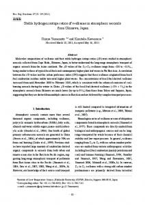
long. In the modern ocean they have been used as tracers for melting of sea ice4, glacial and river run-off, deep ocean water masses5 and deep-water formation processes6. The isotopic compositions at various stages of the hydrological cycle help constrain different water masses and their movement. Isotopic compositions of ice cores have become the most important tools for palaeotemperature reconstructions7,8. The variation in the isotopic composition of deep-sea water is relatively smaller than that in freshwater and mainly determined by freshwater input and mixing between water masses9. Several expeditions have been made earlier to explore the Indian Ocean and the Southern Ocean10–13. But due to high spatial and temporal variability this region needs more studies to characterize its physical (such as temperature and salinity), chemical and isotopic properties adequately. Some studies have shown that due to global warming, parts of Antarctic ice sheet are melting and the Southern Ocean is getting more and more melt water14–17. This makes the isotopic study of the Southern Ocean all the more urgent. Combined study of stable hydrogen (δ D) and oxygen (δ 18O) isotopes and salinity can be ideal to monitor various processes happening in the oceans. Here new δ D and salinity data pertaining to the Indian sector of the Southern Ocean are presented and discussed (details of the oxygen isotope data are presented elsewhere18). About a hundred samples of ocean surface water were collected during the second expedition to the Southern Ocean and Larsemann Hills, Antarctica onboard R/V Akademik Boris Petrov (25 January to 1 April 2006). A vast area (from 13°N to 68°S and 48°E to 77°E) was covered for sampling (Figure 1). Surface sea water samples were collected with the help of a small, clean plastic bucket. Before sample collection, the bucket was rinsed with the surface water of the sampling site. This collected water was stored in 100 ml plastic bottles with tightfitting double caps to prevent evaporation. Bottles were filled up to the brim to facilitate easy identification of any later evaporation/leakage and taped at the neck as a further precaution. Salinity (in Practical Salinity Units, psu) was measured with a salinometer (Autosal) onboard with an accuracy of 0.001‰. When the water temperature was 1395
SPECIAL SECTION: close to 0°C, the salinity measurements were not made (Table 1). A dual-inlet isotope ratio mass spectrometer (PDZEuropa Geo 20-20) was used for isotopic analysis. Equilibration of the water samples was achieved with H2 gas for δ D analysis19. Platinum-coated beads (known as Hoko Beads) were used as catalyst for the equilibration in about two hours. The equilibrated gas was let into the mass spectrometer for isotopic analysis. The isotopic composition is expressed in the conventional units defined by:
δ = [(R/Rstandard ) – 1] × 1000‰, where R = D/H (or 18O/16O). We used VSMOW (Vienna Standard Mean Ocean Water) as a reference20. Standard deviation of the δ D measurement was about ± 1‰. The δ D values of ocean waters are sensitive to variations in the evaporation–precipitation processes. The isotopic compositions of the surface waters of the ocean are determined by the amount of rainfall (precipitation) and the amount of water that evaporates from the ocean. In regions where the amount of precipitation or river run off is higher than evaporation (P > E, negative net evaporation), the ocean surface becomes diluted in the heavier isotopes (D and 18O) and the net isotopic composition becomes lighter. Conversely, a higher rate of evaporation compared to that of precipitation (E > P, positive net evaporation) leads to the enrichment of heavier isotopes.
Figure 1. Cruise track shows locations of sample collection in the Indian Ocean, denoted by stars. 1396
This is due to the preferential removal of lighter isotopes (H and 16O) from the ocean surface. Similarly, a positive net evaporation leads to an increase in salinity, whereas negative net evaporation leads to a decrease in salinity. These processes cause linear relationships between the stable isotopes (δ D and δ 18O) and salinity, the slopes depending on climatic constraints21. At higher latitudes, the effect of freezing at the ocean surface increases salinity as salt is excluded while freezing. However, it causes only a weak depletion in the δ D values of the remaining liquid sea water. This is because the isotopic fractionation between ice and water is much smaller than that between vapour and water. The melting of sea ice causes large changes in salinity and leaves δ D almost unchanged (the resulting mixture may be only slightly enriched in δ D), whereas melting of continentalice causes large drops both in salinity and δ D22. So the combined study of stable isotopic composition (δ D or δ 18O) and salinity provides a unique method to trace ocean surface processes. We observed a large variation in the surface water salinity (from 35.63 to 33.34 psu) throughout the cruise. Near the equator, between 60°E and 70°E, salinity exhibits high and low salinity values very near each other (Figure 2). In the present study 4°S makes a clear demarcation between the evaporation-dominated zone (i.e. high salinity due to positive E–P) and the precipitation dominated zone (i.e. low salinity due to negative E–P). More samples are required from other sites in the same latitude range to confirm the longitudinal extent of this effect.
Figure 2. waters.
Variation of salinity (in practical salinity units) of surface
CURRENT SCIENCE, VOL. 99, NO. 10, 25 NOVEMBER 2010
INDIAN CONTRIBUTION IN SOUTHERN OCEAN Table 1. Station
Latitude (°) Longitude (°E)
1 2 3 4 5 6 7 8 9 10 11 12 13 14 15 16 17 18 19 20 21 22 23 24 25 26 27 29 30 31 32 33 34 35 36 37 38 39 40 41 42 43 44 45 46 47 48 49
13.11 11.96 11.00 9.01 8.03 7.01 5.97 5.00 4.00 2.99 2.00 0.99 0.01 –0.72 –1.01 –1.37 –2.00 –2.99 –3.48 –4.00 –4.54 –5.01 –6.01 –7.00 –7.50 –7.50 –20.17 –20.27 –24.10 –25.03 –26.04 –26.96 –27.98 –29.00 –29.98 –31.04 –32.01 –33.02 –33.99 –34.96 –36.03 –37.00 –38.02 –39.00 –40.04 –41.00 –42.00 –43.00
71.00 70.54 70.02 68.91 68.38 67.84 67.25 66.70 66.21 65.68 65.09 64.60 64.02 63.67 63.51 63.30 62.94 62.42 62.19 61.92 61.59 61.30 60.75 60.22 59.96 60.95 57.35 57.29 57.52 57.51 57.50 57.51 57.50 57.50 57.49 57.50 57.51 57.50 57.50 57.50 57.51 57.50 57.50 57.50 57.50 57.50 57.50 57.50
Stable hydrogen isotopic composition (δ D) and salinity of sea water Salinity (psu*)
δ D (‰)
Station
Latitude (°)
Longitude (°E)
Salinity (psu*)
3.7 4.2 5.0 3.5 3.8 4.3 4.6 4.1 4.0 4.8 4.1 5.5 5.4 6.5 6.0 5.2 7.0 5.5 5.7 5.4 5.5 5.4 4.3 5.7 6.0 6.0 6.3 4.8 4.9 6.5 5.8 6.1 6.4 5.9 5.1 5.0 3.9 4.3 6.2 4.6 5.6 4.2 6.3 3.6 5.1 3.6 1.6 3.8
50 51 52 53 54 55 56 57 58 59 60 61 62 63 64 65 66 67 68 69 70 71 72 73 74 75 76 77 78 79 80 81 82 83 84 85 86 87 88 89 90 91 92 93 94 95 96 97
–43.99 –45.00 –46.05 –47.02 –51.00 –52.02 –53.00 –54.06 –55.04 –56.02 –56.99 –58.00 –59.01 –60.05 –60.98 –62.02 –63.01 –64.04 –65.00 –66.00 –66.99 –68.01 –67.01 –66.34 –65.79 –65.79 –65.66 –65.50 –65.39 –65.23 –65.10 –64.97 –64.82 –64.56 –57.05 –56.00 –54.05 –43.82 –42.87 –42.01 –41.01 –39.00 –37.90 –37.00 –36.00 –35.02 –34.02 –32.99
57.50 57.50 57.50 57.50 58.79 59.51 60.25 61.07 61.86 62.63 63.44 64.30 65.18 66.11 66.97 67.96 68.99 70.03 71.03 72.16 73.95 77.54 71.12 69.06 64.96 64.96 64.00 62.94 62.00 60.99 59.97 58.99 58.01 56.09 49.91 50.01 50.00 49.20 48.12 48.01 48.02 48.00 48.00 48.00 48.00 48.00 48.00 48.00
34.61 33.59 33.57 33.60 33.77 33.77 33.81 33.80 33.76 ND 33.8 33.68 33.75 33.69 33.57 33.82 33.51 33.81 33.97 33.88 33.75 33.40 33.34 ND ND ND ND ND ND ND ND 34.38 ND ND ND ND ND ND ND ND 35.49 35.51 35.54 35.51 35.57 35.53 35.54 ND
ND** ND ND ND ND ND ND 34.91 34.92 35.26 35.28 35.27 35.29 35.35 35.43 ND 35.45 35.45 ND 34.90 ND 34.69 34.62 34.59 34.75 34.73 35.06 ND ND 35.37 35.39 35.47 35.63 35.54 35.52 35.52 35.46 35.44 35.13 35.50 35.49 35.36 35.25 35.16 35.37 35.36 34.67 34.92
δ D (‰) 1.4 –4.3 –3.8 –2.5 –2.6 –3.6 –3.4 –2.3 –1.6 –2.2 –1.8 –1.1 –1.6 –3.2 –3.1 –2.7 –2.5 –1.3 –0.6 –0.8 –1.6 –2.5 –1.1 0.0 –0.7 –0.9 –1.3 –2.0 –2.7 –2.8 –1.2 –2.3 –2.9 –2.0 –2.1 –1.9 –3.2 –2.6 –1.7 –2.3 2.3 5.1 4.2 2.8 4.6 3.6 3.4 4.0
*psu = Practical salinity units; **ND = not determined.
An increase in salinity was observed to the south of 20°S, which reached a maximum of 35.6 psu and constant in the region between 28°S and 41°S. However, it showed a sharp decrease between 41°S and 45°S. This decrease can either be due to (i) heavy precipitation or (ii) underwater current which breaks at the surface. With a small increase of 0.17 psu between 47°S and 51°S, from 51°S onwards salinity shows a decreasing trend with some small fluctuations. This small increase can be CURRENT SCIENCE, VOL. 99, NO. 10, 25 NOVEMBER 2010
due to vertical mixing caused by high winds in this region. Hydrogen isotopic composition follows the same trend as salinity (Figure 3). A sharp decrease at (41°S–45°S) confirms the effect of precipitation or shoaling of an underwater current. Barring some fluctuations, which are within the experimental uncertainties, δ D showed an overall increasing trend, moving towards the south. This increase in the δ D values reflects the increasing effect 1397
SPECIAL SECTION: in situ melting of sea ice. In other words, as we move towards the Antarctic continent the effect of melting/ freezing processes increases. Thus on the basis of salinity and hydrogen isotopic data it is inferred that the Indian Ocean north of 41°S is a zone of dominant evaporation/ precipitation whereas south of 47°S it is dominated by melting/freezing. The region between 41°S and 47°S is a transition zone between the above two regions. A schematic representation of these zones is shown in Figure 4.
Figure 3. Latitudinal variation of δ D (not along a single longitude, involves samples from all locations shown in Figure 1).
Figure 4. Schematic diagram showing different zones in the Southern Indian Ocean, where different hydrological processes dominate.
Figure 5. Plot of δ 18O versus δ D of surface sea water from the Indian Ocean (best fit line with slope = 7.32 ± 0.28, intercept = 0.29 ± 0.14, r2 = 0.88). Global meteoric water line is also shown for comparison. 1398
The relation between δ D and δ 18O of the ocean surface water gives information about the humidity at the time of evaporation. For worldwide fresh surface waters, Craig22 has found that δ 18O and δ D exhibit a linear correlation, which defines the global meteoric water line (GMWL). Its slope is ~ 8 and intercept is ~ 10‰. The slope is ~ 8 because this is approximately the value produced by equilibrium Rayleigh fractionation of evaporating water surface at about 100% humidity. The value of ~ 8 is also close to the ratio of the equilibrium fractionation factors for H and O isotopes at 25–30°C (refs 19, 23, 24). The slope reduces to less than ~ 8 due to evaporation controlled by ambient humidity (and also due to diffusion through the water vapour boundary layer and exchange with atmospheric water vapour) at the ocean surface. The non-equilibrium evaporation process is characterized25–27 by a slope of less than ~ 8. The relation between δ D and δ 18O for the Indian Ocean is depicted in Figure 5, where data points cluster in two distinct bunches. The best fit line has a slope of (7.32 ± 0.28), which is significantly lower than the slope of GMWL (8.12 ± 0.07). This indicates the Southern Ocean as a whole is evaporating under the non-equilibrium condition, with a mean ambient humidity significantly less than 95%, as also borne out by humidity observations during the cruise. As a result, the Indian Ocean samples show an intercept of 0.29 ± 0.11, which is much less than the intercept of GMWL (9.20 ± 0.53). The relation between δ D and δ 18O shows the two end point mixing type of phenomenon (points in the two big circles). This again emphasizes that the region between 41°S and 45°S is a transition region between two different types of zones. In summary in the Southern (Indian) Ocean, the region between 41°S and 45°S makes a demarcation between an evaporation/precipitation zone (north of 41°S) and a melting freezing zone (south to 45°S). The sharpness of the transition zone could be dependent on season. A little lower slope of the δ D–δ 18O line than 8 reveals that evaporation occurs in the Southern Ocean under isotopic non-equilibrium condition, i.e. kinetic effects (due to diffusion-related fractionation) during vapour formation are more prominent. Future studies may throw light on the seasonal and spatial variations in the Southern Ocean. 1. International Hydrographic Organization (http://www.iho.ohi.net/ english/home/), 2000. 2. Park, Y. H., Charriaud, E. and Fieux, M., Thermohaline structure of Antarctic Surface Water/Winter Water in the Indian sector of Southern Ocean. J. Mar. Syst., 1998, 17, 5–23. 3. Gordon, A. L. and Huber, B. A., Thermohaline stratification below the Southern Ocean sea ice. J. Geophys. Res., 1984, 89, 641– 648. 4. Macdonalds, R. W., Carmack, E. C., McLaughlin, F. A., Falkner, K. K. and Swift, J. H., Connections among ice, runoff and atmospheric forcing in Beaufort Gyre. Geophys. Res. Lett., 1999, 26(15), 2223–2226. CURRENT SCIENCE, VOL. 99, NO. 10, 25 NOVEMBER 2010
INDIAN CONTRIBUTION IN SOUTHERN OCEAN 5. Meredith, M. P., Heywood, K. J., Frew, R. D. and Dennis, P. F., Formation and circulation of the water masses between the southern Indian Ocean and Antarctica: results from δ 18O. J. Mar. Res., 1999, 57, 449–470. 6. Jacobs, S. S., Fairbanks, R. G. and Horibe, Y., Origin and evolution of water masses near the Antarctic continental margin: evidence from H218O/H216O ratios in seawater. In Oceanology of the Antarctic Continental Shelf. Antarctic Research Series (ed. Jacobs, S. S.), AGU, Washington, DC, 1985, pp. 59–85. 7. Gat, J. R., Oxygen and hydrogen isotope in hydrologic cycle. Annu. Rev. Earth Planet Sci., 1996, 24, 225–262. 8. Schotterer, U., Oldfield, F. and Frölich, K., Global Network for Isotopes in Precipitation, IAEA, Vienna, 1996, pp. 1–48. 9. Paul, A., Mulitza, S., Pätzold, J. and Wolff, T., In Use of Proxies in Paleoceanography – Examples from the South Atlantic (eds Fischer, G. and Wefer, G.), Springer-Verlag, Berlin, 1999, pp. 655–686. 10. Delaygue, G., Bard, E., Rollion, C., Jouzel, J., Stievenard, M., Duplessy, J.-C. and Ganssen, G., Oxygen isotope/salinity relationship in the northern Indian Ocean. J. Geophys. Res., 2001, 106, 4565. 11. Duplessy, J.-C., Note preliminaire sur les variations de la composition isotopique des eaux superficelles de l’Océan Indien: La relation 18O-Salinité. C.R. Acad. Sci. Paris, 1970, 271, 1075–1078. 12. Kallel, N., La composition isotopique des eaux du secteur indien de l'océan austral, Master’s thesis, Université de Paris Sud, 1985. 13. Archambeau, A. S., Pierrie, C., Poisson, A. and Schauer, B., Distribution of oxygen and carbon stable isotopes and CFC-12 in the water masses of the southern ocean at 30°E from South Africa to Antarctica: results of CIVA1 cruise. J. Mar. Syst., 1998, 17, 25–38. 14. Aoki, S., Yoritaka, M. and Masuyama, A., Multidecadal warming of subsurface temperature in the Indian sector of the Southern Ocean. J. Geophys. Res., 2003, 108, 8081. 15. Aoki, S., Bindoff, N. L. and Church, J. A., Interdecadal water mass changes in the Southern Ocean between 30°E and 160°E. Geophys. Res. Lett., 2005, 32, L07607. 16. Banks, H. T. and Bindoff, N. L., Comparison of observed temperature and salinity changes in the Indo-Pacific with results from the Coupled Climate Model HadCM3: processes and mechanisms. J. Climate, 2002, 16, 156–166.
CURRENT SCIENCE, VOL. 99, NO. 10, 25 NOVEMBER 2010
17. Barnett, T. P., Pierce, D. W., Achuta Rao, K. M., Gleckler, P. J., Santer, B. D., Gregory, J. M. and Washington, W. M., Penetration of human-induced warming into the World’s Oceans. Science, 2005, 309, 284. 18. Srivastava, R., Ramesh, R., Prakash, S., Anilkumar, N. and Sudhakar, M., Oxygen isotope and salinity variations in the Indian sector of the Southern Ocean. Geophys. Res. Lett., 2007, 34, L24603. 19. Gonfiantini, R., The δ-notation and the mass-spectrometric measurement techniques. In Stable Isotope Hydrology: Deuterium and Oxygen-18 in the Water Cycle. Technical Report Series No. 210 (eds Gat, J. R. and Gonfiantini, R.), IAEA, Vienna, 1981, pp. 103– 142. 20. Craig, H., Isotopic standards for carbon and oxygen and correction factors for mass spectrometric analysis of carbon dioxide. Geochim. Cosmochim. Acta, 1957, 12, 133–149. 21. Craig, H. and Gordon, L. I., Stable isotope in oceanographic studies and paleotemperatures. V. Lischi e Figli, Pisa, 1965, 122. 22. Craig, H., Isotopic variations in meteoric waters. Science, 1961, 133, 1702–1703. 23. Kendall, C. and McDonnell, J. (eds), Isotope Tracers in Catchment Hydrology, Elsevier Publisher, Amsterdam, 1998, p. 839. 24. Clark, I. D. and Fritz, P., Environmental Isotopes in Hydrogeology, Levis Publisher, CRC Press, Boca Raton, 1997, p. 328. 25. Gat, J. R., In Stable Isotope Hydrology: Deuterium and Oxygen-18 in the Water Cycle. Technical Report Series No. 210 (eds Gat, J. R. and Gonfiantini, R.), IAEA, Vienna, 1981, pp. 21–33. 26. Mook, W. G., Introduction to Isotope Hydrology: Stable and Radioactive Isotopes of Hydrogen, Oxygen and Carbon, Taylor and Francis, London, 2006. 27. Dansgaard, W., Stable isotopes in precipitation. Tellus, 1964, 16, 436–468.
ACKNOWLEDGEMENTS. We thank the Department of Ocean Development and National Institute Antarctic and Oceanographic Research for opportunity to participate in the expedition to the Southern Ocean. We also thank the captain, chief scientist and the crew of R/V Akademik Boris Petrov. We thank the reviewers for their critical comments.
1399