to thank Ralph Cohen and Steve Kerckhoff, who sat on my area exam and ... Cornell, Ken Brown, Marshall Cohen, and Ravi Ramakrishna; at Stanford, Greg.
STABLE REPRESENTATION THEORY OF INFINITE DISCRETE GROUPS
A DISSERTATION SUBMITTED TO THE DEPARTMENT OF MATHEMATICS AND THE COMMITTEE ON GRADUATE STUDIES OF STANFORD UNIVERSITY IN PARTIAL FULFILLMENT OF THE REQUIREMENTS FOR THE DEGREE OF DOCTOR OF PHILOSOPHY
Daniel A. Ramras July 2007
c Copyright by Daniel A. Ramras 2007
All Rights Reserved
ii
I certify that I have read this dissertation and that, in my opinion, it is fully adequate in scope and quality as a dissertation for the degree of Doctor of Philosophy.
(Gunnar Carlsson) Principal Adviser
I certify that I have read this dissertation and that, in my opinion, it is fully adequate in scope and quality as a dissertation for the degree of Doctor of Philosophy.
(Ralph Cohen)
I certify that I have read this dissertation and that, in my opinion, it is fully adequate in scope and quality as a dissertation for the degree of Doctor of Philosophy.
(Steven Kerckhoff)
Approved for the University Committee on Graduate Studies.
iii
Abstract The goal of this thesis is to study representations of infinite discrete groups from a homotopical viewpoint. Our main tool and object of study is Carlsson’s deformation K-theory, which provides a homotopy theoretical analogue of the classical representation ring. Deformation K-theory is a contravariant functor from discrete groups to connective Ω-spectra, and we begin by discussing a simple model for the zeroth space of this spectrum. We then investigate two related phenomena regarding deformation K-theory: Atiyah-Segal theorems, which relate the deformation K-theory of a group to the complex K-theory of its classifying space, and excision, which relates the deformation K-theory of an amalgamation to the deformation K-theory of its factors. In particular, we use Morse theory for the Yang-Mills functional to prove an Atiyah-Segal theorem for fundamental groups of compact, aspherical surfaces, and we prove that deformation K-theory is excisive on all free products. Combined with work of Tyler Lawson, the former result yields homotopical information about the stable coarse moduli space of surface-group representations.
iv
Acknowledgements I would like to thank my advisor, Gunnar Carlsson, for all of his help and support over the years. He suggested the topic of this thesis, and his encouragement and advice were crucial to my progress. Without his enthusiasm, optimism and confidence, much of this research would never have come to fruition. I would also like to thank Ralph Cohen and Steve Kerckhoff, who sat on my area exam and reading committees. Over the years, various professors have been influential to my development: at Cornell, Ken Brown, Marshall Cohen, and Ravi Ramakrishna; at Stanford, Greg Brumfiel, Ralph Cohen, and Ravi Vakil. I learned Morse theory and Yang-Mills theory from Ralph, which play a large role in this thesis. I also thank R. Friedman, C.-C. Liu, R. Mazzeo, R. Shoen, and K. Wehrheim for helpful conversations. At Stanford, I had the pleasure of learning with and from a great number of fellow topology students and postdocs: David Ayala, Chris Douglas, Soren Galatius, Vero Godin, Kate Gruher, Brian Munson, Brett Parker, Antonio Ramirez, Pete Storm, and especially Tyler Lawson and Robert Lipshitz. Tyler’s patient answers and insightful explanations proved invaluable on many occasions. Robert’s keen insights helped me around many roadblocks in my thinking. My friends and family deserve special thanks. My parents encouraged and nurtured my interest in mathematics from a young age, and my father first introduced me to the beauty of the subject. Gabe, Jordan, Tammy, Robert and Elizabeth helped keep me sane through the trials of graduate school. Most of all I must thank Gin, whose love, companionship, and unwavering support kept me going. Without her, this thesis could never have been written.
v
The appendix was expertly typed by Bob Hough. Portions of this thesis were written during visits to Columbia University, and I would like to thank the Columbia mathematics department for its hospitality. During my time at Stanford I was funded by both an NDSEG fellowship, from the Department of Defense, and later an NSF fellowship.
vi
Contents Abstract
iv
Acknowledgements
v
1 Introduction
1
2 Deformation K-theory: basic properties
7
3 Group completion in deformation K-theory
13
4 An Atiyah-Segal theorem for surface groups
30
4.1
Group completion for surface groups . . . . . . . . . . . . . . . . .
33
4.2
Representations, flat connections, and semi-stable bundles . . . . .
35
4.3
The Harder-Narasimhan stratification . . . . . . . . . . . . . . . . .
45
4.4
Proof of the Atiyah-Segal theorem for surface groups . . . . . . . .
55
4.5
Stable representation spaces . . . . . . . . . . . . . . . . . . . . . .
59
4.6
The stable coarse moduli space . . . . . . . . . . . . . . . . . . . .
68
4.7
Free products . . . . . . . . . . . . . . . . . . . . . . . . . . . . . .
71
5 Excision in deformation K-theory
75
5.1
Excision for free products . . . . . . . . . . . . . . . . . . . . . . .
79
5.2
Reduction of excision to representation varieties, and an example
86
.
6 Examples
98
6.1
Surface-type groups . . . . . . . . . . . . . . . . . . . . . . . . . . .
6.2
Finitely generated abelian groups . . . . . . . . . . . . . . . . . . . 111
vii
99
A Holonomy of flat connections
114
Bibliography
133
viii
List of Figures 3.1
A loop γ and its normalization N(γ). . . . . . . . . . . . . . . . . .
22
4.1
The convex path P ((1, 3), (2, 2), (4, 1), (4, −1), (1, −5)). . . . . . . .
47
A.1 Basepoints and holonomy. . . . . . . . . . . . . . . . . . . . . . . . 120
ix
Chapter 1 Introduction Associated to any discrete group Γ, one has the (unitary) representation ring R(Γ), which consists of “virtual isomorphism classes” of representations. To form R(Γ), one starts with the sets Hom(Γ, U(n)), and kills the conjugation action of U(n). Block sum of unitary matrices makes the collection of these sets, as n varies, into an abelian monoid, and R(Γ) is the Grothendieck group of this monoid. Hence R(Γ) consists of formal differences between (isomorphism classes of) representations. This process completely ignores the fact that the sets Hom(Γ, U(n)) have a natural topology, coming from the topology on the groups of unitary matrices. To be precise, one may take the compact-open topology, or (equivalently) the topology coming from the embedding Hom(Γ, U(n)) ֒→ U(n)S , where S ⊂ Γ is any generating set. For finite groups Γ, the space Hom(Γ, U(n)) is, topologically speaking, easily understood. The trace of a representation gives a continuous, complete invariant of the isomorphism type, and the trace can take on only countably many values. Hence two non-isomorphic representations are never connected by a path, and since U(n) is connected any two isomorphic representations ρ and AρA−1 are connected by a path. Hence the component of the representation space containing a given representation ρ is simply the orbit U(n)/Stab(ρ), and basic representation theory shows that Stab(ρ) is a product of smaller unitary groups (whose dimensions record the degree with which each irreducible appears in ρ). In particular, when Γ is finite the space Hom(Γ, U(n)) depends, topologically speaking, only on the number and dimension of the irreducible representations of Γ. 1
CHAPTER 1. INTRODUCTION
2
In contrast, it is well-known that for any Riemann surface M g , the representation spaces Hom(π1 (M g ), U(n)) are connected (see Corollary 4.3.8) and carry a great deal of information. Thus one is inclined to look for an analogue of the representation ring which captures the topology of the representation spaces. As we will discuss, one specific motivation is the desire to prove Atiyah-Segal theorems relating representations of an infinite discrete group Γ to the complex K-theory of the classifying space BΓ. Carlsson’s deformation K-theory spectrum, first introduced in [10], is precisely the sort of object we want. Its construction may be viewed as the homotopy theoretical analogue of the construction of the representation ring. To form the deformation K-theory spectrum of a discrete group Γ, we replace each step in the construction of R(Γ) by its homotopy theoretical analogue. We begin by taking the spaces Hom(Γ, U(n)), and rather than modding out conjugation, we form the homotopy quotients, or homotopy orbit spaces, Hom(Γ, U(n))hU (n) := EU(n) ×U (n) Hom(Γ, U(n)) (Here EU(n) denotes the total space of a universal, principal U(n)-bundle. We will frequently use the notation XhG for EG ×G X, where G is a topological group acting on a space X.) These homotopy orbit spaces form a topological monoid Rep(Γ)hU under block sum, and the deformation K-theory of Γ is the homotopy group completion of this monoid. More precisely, as we explain below, Rep(Γ)hU is the classifying space of a topological permutative category, and deformation Ktheory is the associated K-theory spectrum. (This version of deformation K-theory was first described in Lawson’s thesis [29].) The first two homotopy groups of Kdef (Γ) have rather direct meanings. In 0 dimension zero, the group Kdef (Γ) is the group of “virtual path components” of
representations, i.e. formal differences [ρ1 ]−[ρ2 ], where ρi ∈ Hom(Γ, U(ni )) for some ni and square brackets denote path components. This elementary fact is proven in 1 Lemma 2.0.5. The group Kdef (Γ) is essentially a version of π1 (Hom(Γ, U(n))/U(n)),
stabilized with respect to rank. A precise result along these lines is proven in Proposition 4.6.1, using a theorem of Lawson regarding the Bott map in deformation
3
CHAPTER 1. INTRODUCTION
K-theory [30]. ∗ Thus far, there have been relatively few computations of the groups Kdef (Γ) for Γ
an infinite discrete group. Lawson [30] has provided computations for free groups, as well as a product formula [31] computing Kdef (Γ1 × Γ2 ) in terms of Kdef (Γ1 ) and Kdef (Γ2 ), as modules over the connective K-theory spectrum ku. Specifically, Lawson has shown that there is a weak equivalence of ku-modules Kdef (Γ1 × Γ2 ) ≃ Kdef (Γ1 ) ∧ Kdef (Γ2 ). ku
(1.1)
The results of this thesis add to the list of computations: Theorem 4.4.1 provides ∗ a complete calculation of Kdef (π1 (Σ)), for any compact, aspherical surface Σ, and
Theorem 4.7.5 computes the deformation K-theory of a free product Γ1 ∗ Γ2 in terms of the deformation K-theory of Γ1 and Γ2 . The results of this thesis focus on three topics in deformation K-theory: group completion (Chapter 3), which provides, under suitable conditions, convenient models for the zeroth space of the deformation K-theory spectrum; Atiyah-Segal theorems (Chapter 4), which relate Kdef (Γ) to complex K-theory of the classifying space BΓ; and excision (Chapter 5), which studies the behavior of deformation K-theory on amalgamated products of groups. We proceed to explain these topics in greater detail. The Group Completion Theorem [8, 16, 33] provides a homological model for the group completion ΩBM of a topological monoid M. In Chapter 3, we provide conditions (Theorem 3.0.11) under which this homological model actually has the same (weak) homotopy type as the group completion, rather than just the same homology. Furthermore, these conditions are satisfied quite generally for deformation K-theory, and this provides us with a model for the homotopy type of the zeroth space of the spectrum Kdef (Γ) (Corollary 3.0.16). This model is crucial for the excision results in Chapter 5. We also use this result (or rather special cases of it) in Chapter 4, both as the starting point for our Atiyah-Segal theorem, and in our results on the stable coarse moduli space of representations. The classical theorem of Atiyah and Segal [7] states that for a compact Lie
CHAPTER 1. INTRODUCTION
4
group Γ, the complex K-theory of the classifying space BΓ is isomorphic to the completion of the representation ring R(Γ) (at the augmentation ideal). A central goal of this thesis is to provide an analogue of this result, relating the deformation K-theory of π1 Σ, where Σ is a compact, aspherical surface, to the complex Ktheory of Σ itself. Since Σ is aspherical, we have Σ = B (π1 Σ), so this is indeed an analogue of the Atiyah-Segal theorem. More precisely, we prove in Theorem 4.4.1 that there is an isomorphism ∗ Kdef (π1 (Σ)) ∼ = K ∗ (Σ);
in the orientable case, we require ∗ > 0. (We note that Lawson’s product formula (1.1) provides an alternate proof in the genus 1 case, since in this case π1 Σ = Z × Z.) Using similar methods, we also study the representation spaces themselves (Section 4.5), obtaining in particular the homotopy type of the stable representation space Hom(π1 Σ, U) and the connectivity of the inclusions Hom(π1 Σ, U(n)) ֒→ Hom(π1 Σ, U(n + 1)). Furthermore, combining our results with Lawson’s work on the Bott map in deformation K-theory [30], we obtain results regarding the “stable coarse moduli space” Hom(π1 Σ, U)/U (Section 4.6). The proofs of these results rely on Morse theory for the Yang-Mills functional, as developed by Atiyah and Bott [6], Daskalopoulos [12], and R˚ ade [40]. (The key analytical input comes from Uhlenbeck’s compactness theorem [47, 48].) The link between deformation K-theory and Yang-Mills theory is provided by the wellknown fact that representations of the fundamental group induce flat connections, which form a critical set for the Yang-Mills functional. In Chapter 5, we discuss the question of excision in deformation K-theory. Given an amalgamated product of groups, one may apply deformation K-theory to obtain a square of spectra, and we say that deformation K-theory is excisive on the amalgamated product if this diagram of spectra is homotopy cartesian. Our main result, Theorem 5.1.1, shows that deformation K-theory satisfies excision for all free products. The proof depends crucially on the group completion results from
CHAPTER 1. INTRODUCTION
5
Chapter 3. For more general amalgamated products, excision may fail in low dimensions. In Section 5.1, we show that the fundamental group of a Riemann surface, described as an amalgamated product via a connected sum decomposition of the surface, fails to satisfy excision on π0 (we expect that the natural map φ induces an isomorphism in positive degrees, though; see Conjecture 5.0.7). In Section 5.2, we offer several results regarding more general amalgamated products: we show how to deduce excision results in deformation K-theory from stable information about the representation spaces themselves (Proposition 5.2.4), and we study excision in low dimensions for some specific examples of amalgamated products (Proposition 5.2.5). We conclude Section 5.2 by describing a technique, involving stratified fibrations, which we hope will be useful in further work on excision. It is interesting to note that excision and Atiyah-Segal theorems are closely related phenomena. This is due to the fact that complex K-theory is a cohomology theory, and in particular satisfies excision. More precisely, consider an amalgamated product G ∗K H in which the maps K → G and K → H are injective. Then the classifying space B(G ∗K H) is the homotopy pushout of the diagram BG ←− BK −→ BH, and hence one has a long-exact Mayer-Vietoris sequence in complex K-theory. Given Atiyah-Segal theorems relating deformation K-theory of the factors G, K, and H to the K-theory of their classifying spaces, one then expects that an Atiyah-Segal theorem for G ∗K H will be equivalent to excision (in deformation Ktheory) for this amalgamated product. More precisely, if the square of deformation K-theory spectra associated to G ∗K H is homotopy cartesian, then one has a Mayer-Vietoris sequence in deformation K-theory as well as in topological K-theory, ∗ and an isomorphism between Kdef (G ∗K H) and K ∗ (B(G ∗K H)) should follow
from the 5-lemma; on the other hand, if one has an Atiyah-Segal theorem relating ∗ Kdef (G ∗K H) to K ∗ (B(G ∗K H)), then the Mayer-Vietoris sequence in complex K-
theory should correspond to a Mayer-Vietrois sequence in deformation K-theory, allowing one to prove excision. The difficulty here, as the reader may have guessed,
CHAPTER 1. INTRODUCTION
6
is naturality. In order to transfer information between deformation K-theory and topological K-theory, one needs a natural transformation connecting the functor Kdef (−) to the function spectrum F (B(−), ku). Although we describe one such natural transformation in Chapter 2, it is not known to be an equivalence in any interesting cases. In particular, the known Atiyah-Segal theorems involve very different maps, and in interesting cases such as connected sum decompositions of Riemann surfaces, these maps are not natural with respect to the amalgamated product structures. The final chapter of this thesis focuses on examples. In particular, we consider several families of groups in which the group completion results from Chapter 3 apply, yielding explicit models for the zeroth space of deformation K-theory. In 0 addition, we compute the group Kdef in most of these cases. These results rely
heavily on work of Ho and Liu [24, 25], who designed a simple obstruction theory for studying path components of representation spaces and paired it with the theory of quasi-Hamiltonian moment maps [4] in order to compute π0 Hom(π1 Σ, G) for (most) surfaces Σ and any compact, connected Lie group G. We specialize their work to the case of the unitary groups, where some simplifications are possible, and then extend their arguments to “surface-type groups,” that is, groups with presentations similar to surface groups (Theorem 6.1.9). Proposition 6.1.11 discusses a family of groups related to the Klein bottle, and finitely generated abelian groups are discussed in Proposition 6.2.2. In an appendix, we discuss the results regarding holonomy of flat connections that are needed in Chapter 4. These results are probably well-known, but no written account seems to be available.
Chapter 2 Deformation K-theory: basic properties
In this chapter, we introduce Carlsson’s notion of deformation K-theory and discuss its basic properties. Deformation K-theory is a contravariant functor from discrete groups to spectra, and is meant to capture homotopy-theoretical information about the representation spaces of the group in question. We will construct a connective Ω-spectrum Kdef (G) by considering the K-theory of an appropriate permutative topological category of representations (this category was first introduced by Lawson [29]). Although we phrase everything in terms of the unitary groups U(n), all of the constructions, definitions and results in this section are valid for the general linear groups GLn (C), and only notational changes are needed in the proofs. For the rest of this section, we fix a discrete group G. Definition 2.0.1 Associated to G we have a topological category R(G) with object space Ob(R(G)) =
∞ a
n=0
7
Hom(G, U(n))
CHAPTER 2. DEFORMATION K-THEORY: BASIC PROPERTIES
8
and morphism space Mor(R(G)) =
∞ a
U(n) × Hom(G, U(n)).
n=0
The domain and codomain maps are dom(A, ρ) = ρ and codom(A, ρ) = AρA−1 , and composition is given by (B, AρA−1 ) ◦ (A, ρ) = (BA, ρ). The representation spaces are topologized using the compact-open topology, or equivalently as subQ spaces of g∈S U(n), where S ⊂ G is any generating set. We define U(0) to be the trivial group, and the single point ∗ ∈ Hom(G, U(0)) will serve as the basepoint.
The functor ⊕ : R(G) × R(G) → R(G) defined via block sums of unitary matrices is continuous and strictly associative, with the trivial representation ∗ ∈ Hom(G, U(0)) as unit, and this functor makes R(G) into a permutative category in the sense of [32]. The natural commutativity isomorphism ∼ =
c : ρ ⊕ ψ −→ ψ ⊕ ρ is defined via the (unique) permutation matrices τn,m satisfying −1 τn,m (A ⊕ B)τn,m =B⊕A
for all A ∈ U(n) and B ∈ U(m). (A general discussion of the functor associated to a collection of matrices like this one can be found in the proof of Corollary 3.0.16.) Any homomorphism f : G → H induces a functor f ∗ : R(H) → R(G) in the obvious manner, and it is easy to check that this functor is permutative. May’s machine [32] constructs a (special) Γ-category (in the sense of [42]) associated to any permutative (topological) category C. Taking geometric realizations yields a special Γ-space, and Segal’s machine then produces a connective Ω-spectrum K(C), the K-theory of the permutative category C. This entire process is functorial in the permutative category C. Definition 2.0.2 Given a discrete group G, the deformation K-theory spectrum
CHAPTER 2. DEFORMATION K-THEORY: BASIC PROPERTIES
9
of G is defined to be the K-theory spectrum of the permutative category R(G), i.e. Kdef (G) = K(R(G)). This spectrum is contravariantly functorial in G. We now describe the zeroth space of the spectrum Kdef (G). Lemma 2.0.3 For any discrete group G, the zeroth space of Kdef (G) is naturally weakly equivalent to ΩB(|R(G)|), where B denotes the bar construction on the topological monoid |R(G)|. The proof of this result is just an elaboration of the proof in [32] that the Γcategory associated to a permutative category C is special. May constructs levelwise maps [32, Construction 10, Step 2] from B(|C|) to the first space of the K-theory spectrum of C. One checks that these fit together into a simplicial map, which is a levelwise weak-equivalence. (May also constructs a sequence of maps in the other direction, but they do not form a simplicial map. Nevertheless, levelwise they provide homotopy inverses, showing that our map is a levelwise weak-equivalence.) Since the identity element of R(G) is disjoint, these simplicial spaces are good and this levelwise equivalence is a weak-equivalence on classifying spaces. Next, we discuss an observation due to Lawson [29] regarding the classifying space of the category R(G). For convenience of the reader, and to set notation, we include a discussion of the simplicial constructions of the classifying space BU(n) and the universal bundle EU(n). Associated to G we have the homotopy orbit spaces Hom(G, U(n))hU (n) = EU(n) ×U (n) Hom(G, U(n)), where EU(n) denotes the total space of a universal principal U(n)-bundle. In fact, we take EU(n) to be the classifying space of the translation category U(n) of U(n), that is, the topological category whose object space is U(n) and whose morphism space is U(n) × U(n). (The morphism (A, B) is the unique morphism from B to A in U(n).) This category admits a right action by U(n) via right
CHAPTER 2. DEFORMATION K-THEORY: BASIC PROPERTIES
10
multiplication; the induced action on kth level of the nerve of U(n) may be written (A1 , . . . , Ak ) · g = (A1 g, . . . Ak g). We define BU(n) to be the classifying space of the topological category CU (n) with one object and with morphism space U(n). The natural functor U(n) → CU (n) sending the morphism (A, B) to AB −1 ∈ U(n) gives a map EU(n) → BU(n) making EU(n) a universal principal U(n) bundle (see [41]). The continuous block sum maps ⊕ : U(n) × U(m) → U(n + m) extend to maps EU(n) × EU(m) → EU(n + m), and allow us to define a monoid structure on the disjoint union ∞ a
Hom(G, U(n))hU (n) =
n=0
∞ a
EU(n) ×U (n) Hom(G, U(n)),
n=0
which we (abusively) denote by Rep(G)hU . Lawson’s observation, then, is: Proposition 2.0.4 (Lawson) The topological monoids |R(G)| and Rep(G)hU are isomorphic. Proof. We begin by considering Hom(G, U(n)) as a constant simplicial space, so that
EU(n) × Hom(G, U(n)) ∼ = k 7→ U(n)k+1 × Hom(G, U(n) .
Now, combining the level-wise action of U(n) on EU(n) with the conjugation action of U(n) on Hom(G, U(n)) gives the simplicial space on the right a simplicial action of U(n), and we have a homeomorphism � EU(n) ×U (n) Hom(G, U(n)) ∼ = k 7→ U(n)k+1 × Hom(G, U(n) /U(n) .
We will now describe a simplicial map from the right hand side to NR(G). We will write Nk R(G), the space of k-tuples of composable morphisms, as ∞ a
U(n)k × Hom(G, U(n))
n=0
where (Ak , . . . , A1 , ρ) is considered as the string of morphisms A
A
A
1 2 k −1 −1 ρ −→ A1 ρA−1 1 −→ . . . −→ Ak · · · A1 ρA1 · · · Ak .
CHAPTER 2. DEFORMATION K-THEORY: BASIC PROPERTIES
11
Then we have a map U(n)k+1 × Hom(G, U(n)) −→ U(n)k × Hom(G, U(n)), given by −1 −1 −1 (Ak+1 , . . . , A1 , ρ) 7→ (Ak+1 A−1 k , Ak Ak−1 , . . . , A2 A1 , A1 ρA1 ).
It is easy to check that this map is simplicial and factors through the U(n)-action on the left, inducing a level-wise homeomorphism from the quotient. Hence we have the desired homeomorphism Hom(G, U(n))hU ∼ = |R(G)| , and since both monoid structures arise from block sum, it is immediate from the definitions that this map is a homomorphism of monoids.
2
We end this section with a simple observation regarding the zeroth homotopy group of deformation K-theory. The topological monoid Rep(G) is defined by Rep(G) =
∞ a
Hom(G, U(n)).
n=0
The monoid structure on Rep(G) is given by block sum of representations (again, U(0) is the trivial group and the single element in Hom(G, U(0)) will act as the identity). The same construction may be applied with the general linear groups in place of the unitary groups, and we keep the notation intentionally vague. 0 Lemma 2.0.5 Let G be a discrete group. Then Kdef (G) ∼ = Gr(π0 (Rep(G))), where
Gr denotes the group-completion of a monoid, i.e. its Grothendieck group. 0 Proof. By Lemma 2.0.3 and Proposition 2.0.4, we know that Kdef (G) is the group
completion of the monoid π0 (Rep(G))hU , so we just need to show that there is an isomorphism of monoids π0 (Rep(G))hU ∼ = π0 (Rep(G)). But the monoid ∞ a
EU(n) × Hom(G, U(n))
n=0
fibers over both sides, with connected fibers.
2
CHAPTER 2. DEFORMATION K-THEORY: BASIC PROPERTIES
12
We conclude this section by considering the general relationship between deformation K-theory of a group G and complex K-theory of the classifying space BG. η
Given a natural transformation Kdef (−) → Map(B(−), ku) and an amalgamated product G ∗K H, we may use η, to compare the square of deformation K-theory spectra associated to G ∗K H with the square of mapping spectra associated to the classifying spaces of the factors. When the maps from K to G and H are injective, the square of classifying spaces is homotopy co-cartesian [20, p. 92], and hence the square of mapping spectra is homotopy cartesian (i.e. complex K-theory is excisive). Thus if η is an isomorphism on homotopy (in a range) for G, H, and K, then it is an isomorphism (in a range) for G ∗K H as well. In the other direction, if η is an isomorphism for G ∗K H as well, then excision for complex K-theory implies excision for deformation K-theory. This is relationship, alluded to in the introduction, between Atiyah-Segal theorems and excision. We briefly describe one such natural transformation η; unfortunately it is not currently known to be an isomorphism on homotopy in any interesting cases (for free groups and surface groups, the isomorphisms arise in completely different manners). e The category R(G) sits inside a larger permutative category R(G), whose objects
are representations and whose morphisms are all (possibly non-equivariant) linear isomorphisms of the underlying vector spaces. This category has a permutative
G-action, which is trivial on objects and sends a morphism A : ρ → ψ to the morphism ρ(g)Aψ(g)−1 : ρ → ψ. G ∼ e The fixed point category of this action is precisely R(G); thus K(R(G)) = e Kdef (G). Now R(G) is equivalent (as a permutative category) to the full subcate-
gory of trivial representations, on which G acts trivially. Hence the homotopy fixed hG e point spectrum K(R(G)) maps by a weak equivalence to kuhG ≃ Map(BG, ku).
Chapter 3 Group completion in deformation K-theory
The goal of this section is to provide a convenient homotopy theoretical model for the group completion of a topological monoid satisfying certain simple properties. The results of this section will be applicable to deformation K-theory, and form the basis of our excision results. In addition, special cases of our main results (Theorem 3.0.11 and Corollary 3.0.16) appear in the computation in Chapter 4 of ∗ Kdef (π1 (Σ)) for compact, aspherical surfaces Σ, and in the related results regarding
Hom(π1 Σ, U)/U. The models for group completion that we will study arise as mapping telescopes, as in [33]. Throughout this section M will denote a homotopy commutative topological monoid and e ∈ M will denote the identity element. We write the operation in M as ⊕, and for any m ∈ M we denote the n-fold product of m with itself by mn . Definition 3.0.6 For any m ∈ M, we denote the mapping telescope ⊕m
⊕m
⊕m
hocolim(M | −→ M −→ {z · · · −→ M}) N
13
CHAPTER 3. GROUP COMPLETION IN DEFORMATION K-THEORY
14
by MN (m), and we denote the infinite mapping telescope ⊕m
⊕m
colim MN (m) = hocolim(M −→ M −→ · · · ) N →∞
by M∞ (m). We denote points in these telescopes by triples (x, n, t), where x ∈ M, n ∈ N and t ∈ [0, 1). Note that each of these spaces is functorial in the pair (M, m) and naturally based by the point (e, 0, 0), which we will denote simply by e. Definition 3.0.7 We say that M is stably group-like with respect to an element m ∈ M if the cyclic submonoid of π0 (M) generated by m is cofinal. In other words, M is stably group-like with respect to m if for every x ∈ M there exists y ∈ M and n ∈ N such that x ⊕ y and mn lie in the same path component of M. We refer to such y as stable homotopy inverses for x (with respect to m). The reason for our terminology is the following result. Proposition 3.0.8 Assume M is homotopy commutative and let m ∈ M be any element. Then there is a natural (abelian) monoid structure on π0 (M∞ (m)), and M is stably group-like with respect to m if and only if π0 (M∞ (m)) is a group under this multiplication. In fact, if M is stably group-like with respect to m, then π0 (M∞ ) is the group completion (i.e. the Grothendieck group) of π0 (M). Proof. First we describe the monoid structure on π0 (M∞ (m)). Given components C1 and C2 in π0 (M∞ (m)) we may choose representatives (x1 , n1 , 0) and (x2 , n2 , 0) for C1 and C2 respectively. Then we define C1 ⊕ C2 to be the component containing (x1 ⊕ x2 , n1 + n2 , 0). To see that this operation is well-defined, note that if (x, n, 0) and (x′ , n′ , 0) are connected by a path, then this path lies in some finite telescope MN (m) (with N > n, n′ ) and one can collapse the first N mapping cylinders co′
ordinates to obtain a path in M from x ⊕ mN −n to x′ ⊕ mN −n . Hence given any other component, represented by a point (y, k, 0), there is a sequence of paths (x ⊕ y, n + k, 0) ∼ (x ⊕ y ⊕ mN −n , N + k, 0) ∼ (x ⊕ mN −n ⊕ y, N + k, 0)
CHAPTER 3. GROUP COMPLETION IN DEFORMATION K-THEORY
15
∼ (x′ ⊕ mN −n ⊕ y, N + k, 0) ∼ (x′ ⊕ y, n′ + k, 0) ′
as desired. This operation is clearly associative and commutative, with the component of (e, 0, 0) as a unit. Now, say M is stably group-like with respect to m ∈ M. Then given any component C of M∞ (m), we choose a representative (x, n, 0) for C and a stable homotopy inverse y for x. Then if x⊕y ∼ mN , one easily checks that the component of (y, N − n, 0) is an inverse for C (we may assume, of course, that N > n). Conversely, if π0 (M∞ (m)) is a group, then for any x ∈ M choose a representative (y, n, 0) for the inverse to the component containing (x, 0, 0). Then (x ⊕ y, n, 0) lies in the same component as (mn , n, 0) and hence (by collapsing cylinders) we may construct a path in M from x ⊕ y ⊕ mk to mn+k for some k. Thus y ⊕ mk is a stable homotopy inverse for x. Next we discuss group completions. There is a natural map φ : π0 (M) → π0 (M∞ (m)), given by φ([x]) = [x, 0, 0] (where square brackets denote the path components containing these points). We must show that a diagram of monoids π0 (M)
f
/
NNN NNNφ NNN N&
GO
f˜
π0 (M∞ (m))
can be completed uniquely whenever G is a group. Consider any component [x, n, t] = [x, n, 0] ∈ π0 (M∞ (m)). We may write [x, n, 0] ⊕ [m, 0, 0]n = [x ⊕ mn , n, 0] = [x, 0, 0] and hence we are forced to define ˜ f˜([x, n, 0]) = f([x, 0, 0]) · f˜([m, 0, 0])−n = f ([x]) · f ([m])−n .
(3.1)
It is easy to check that formula (3.1) gives a well-defined function f˜, and it follows from homotopy commutativity that f˜ is a morphism of monoids. 2 Example 3.0.9 If M is homotopy commutative and π0 (M) is finitely generated,
CHAPTER 3. GROUP COMPLETION IN DEFORMATION K-THEORY
16
with generators m1 , . . . , mk ∈ M, then M is stably group-like with respect to m = m1 ⊕ . . . ⊕ mk : any component is represented by a word in the mi , and we may add another word to even out the powers. (This example appears, in spirit at least, in [33], and will be central to our results on excision.) Before stating the main result of this section, we need the following definition. Definition 3.0.10 Let (M, ⊕) be a homotopy commutative monoid. We call an element m ∈ M anchored if there exists a homotopy H : M × M × I → M such that for every m1 , m2 ∈ M, H0 (m1 , m2 ) = m1 ⊕ m2 , H1 (m1 , m2 ) = m2 ⊕ m1 , and Ht (mn , mn ) = m2n for all t ∈ I and all n ∈ N. Theorem 3.0.11
Let M be a homotopy commutative monoid which is stably
group-like with respect to a anchored element m ∈ M. Then there is a natural isomorphism ∼ =
η : π∗ M∞ (m) −→ π∗ ΩBM, and the induced map on π0 is an isomorphism of groups. The map η is induced by a zig-zag of natural weak equivalences. A number of comments are in order regarding zig-zags, basepoints, and finally, the precise meaning of naturality. First, though, we note that even in the case where M is strictly commutative, this result seems non-obvious (although our proof is hardly difficult in this case). This case will be used later, in our calculation of π1 Hom(π1 Σ, U)/U for compact, aspherical surfaces Σ (Section 4.6). By a zig-zag we simply mean a sequence of spaces X1 , X2 , . . . , Xk , together with maps fi between Xi and Xi+1 (in either direction). The sequence of spaces appearing in our natural zig-zag will be made explicit in the proof. A map f : X → Y between possibly disconnected spaces will be called a weak equivalence if and only if it induces isomorphisms f∗ : π∗ (X, x) → π∗ (Y, f (x)) for all x ∈ X. To prove Theorem 3.0.11, we will exhibit a natural zig-zag of weak equivalences between M∞ (m) and ΩBM. The isomorphism on homotopy groups will then be valid for all compatible choices of basepoint, in the following sense. The zig-zag of isomorphisms on π0 gives an isomorphism η0 : π0 M∞ (m) → π0 ΩBM, and we call
CHAPTER 3. GROUP COMPLETION IN DEFORMATION K-THEORY
17
basepoints x ∈ M∞ (m) and y ∈ ΩBM compatible if η0 ([x]) = [y]. Now, for any compatible basepoints x and y there is in fact a canonical isomorphism ∼ =
ηx,y : π∗ (M∞ (m), x) −→ π∗ (ΩBM, y) . This isomorphism is constructed using the fact that if X is a simple space, meaning that the action of π1 (X, x) on πn (X, x) is trivial for every n > 1, then any two paths between points x1 , x2 ∈ X induce the same isomorphism π∗ (X, x1 ) → π∗ (X, x2 )). Since we are dealing with a zig-zag of weak equivalences ending with a simple space, all spaces involved are simple, and hence ηx,y is well-defined. Naturality means that given a map f : M → N of monoids with are stably group-like with respect to anchored elements m ∈ M and f (m) ∈ N, then for any compatible basepoints x ∈ M∞ (m) and y ∈ ΩBM, we have ΩBf ◦ ηx,y = f∞ ◦ ηf∞ (x),(ΩBf )(y) : π∗ (M∞ (m), x) −→ π∗ (ΩBN, (ΩBf )(y)) , where f∞ = f∞ (m) denotes the map on telescopes induced by f . This equation follows easily from naturality of the weak equivalences involved in the zig-zag. Remark 3.0.12 It is possible to relax the definition of “anchored” with out affecting Theorem 3.0.11 (and only minor changes are needed in the proof ). For example, the homotopies anchoring mn need not be the same for all n, and in fact we only need to assume their existence for “enough” n. (In particular, it is not necessary to assume that there is a homotopy anchoring m0 = e.) For all our applications, though, the current definition suffices. Before beginning the proof, we discuss the application to deformation K-theory. We work mainly in the unitary case, but all of the results are valid in the general linear case as well (and we have noted the places in which the arguments differ). For applications to deformation K-theory, our real interests lie in the monoid of homotopy orbit spaces Rep(G)hU =
∞ a
n=0
Hom(G, U(n))hU (n) ,
CHAPTER 3. GROUP COMPLETION IN DEFORMATION K-THEORY
18
but we can often work with the simpler monoid Rep(G) instead. Note that the spaces EU(n) are naturally based: recall from Section 2 that EU(n) is the classifying space of a topological category whose object space is U(n); the object In ∈ U(n) provides the desired basepoint ∗n ∈ EU(n). These basepoints behave correctly with respect to block sums, i.e. ∗n ⊕ ∗m = ∗n+m . Lemma 3.0.13 Let G be a discrete group. Then Rep(G) is stably group-like with respect to ψ ∈ Hom(G, U(m)) if and only if Rep(G)hU is stably group-like with respect to [∗m , ψ] ∈ Hom(G, U(m))hU (m) . Proof. Say Rep(G) is stably group-like with respect to ψ ∈ Hom(G, U(m)). Then given any [e, ρ] ∈ Rep(G)hU (with e ∈ EU(n) and ρ : G → U(n) for some n) we know that there is a representation ρ−1 : G → U(k) such that ρ ⊕ ρ−1 lies in the component of the ψ l (the l-fold block sum of ψ with itself), where l =
n+k . m
Now, for any e′ ∈ EU(k), the point [e′ , ρ−1 ] is a stable homotopy inverse for [e, ρ] (with respect to ψ), since there is a path in EU(n + k) × Hom(G, U(n + k)) from [e ⊕ e′ , ρ ⊕ ρ−1 ] to [∗n+k , ψ l ]. Conversely, if Rep(G)hU is stably group-like with respect to [∗m , ψ], then any element [e, ρ] ∈ Hom(G, U(n))hU (n) has a stable homotopy inverse [e′ , ρ−1 ] ∈ Hom(G, U(k))hU (k) (for some k), i.e. there is a path in Hom(G, U(n + k))hU (n+k) from [e ⊕ e′ , ρ ⊕ ρ−1 ] to [∗n+k , ψ l ] (where again l =
n+k ). m
Path-lifting for the fibration EU(n + k) ×
Hom(G, U(n + k)) → Hom(G, U(n + k))hU (n+k) produces a path in EU(n + k) × Hom(G, U(n + k)) from (e ⊕ e′ , ρ ⊕ ρ−1 ) to some point (∗n+k · A, A−1 ψ l A), with A ∈ U(n + k). The second coordinate of this path, together with connectivity of U(n), shows that ρ ⊕ ρ−1 lies in the component of ψ l , i.e. ρ−1 is in fact a stable homotopy inverse for ρ (with respect to ψ).
2
We will now show that in deformation Rep(G)hU , elements are always anchored. First we need some lemmas regarding the unitary and general linear groups, which are probably well-known.
CHAPTER 3. GROUP COMPLETION IN DEFORMATION K-THEORY
19
Lemma 3.0.14 Consider an element D = λ1 In1 ⊕ · · · ⊕ λk Ink ∈ GLn (C), where P n = ni and the λi are distinct. Then the centralizer of D in GLn (C) is the
subgroup GL(n1 )×· · ·×GL(nk ), embedded in the natural manner. As a consequence,
the analogous statement holds for the unitary groups. Proof. Say K = [kij ] commutes with X = [xij ], where xij = 0 unless i = j. Letting ei denote the ith standard basis vector, the formula KXei = XKei expands to give Pn Pn j=1 kij xii ej = j=1 kij xjj ej , which precisely states that kij = 0 unless xii = xjj . 2
Lemma 3.0.15 Let K ⊂ GLn (C) be any subgroup. Then the set of diagonalizable matrices in the centralizer C(K) is connected. Similarly, for any K ⊂ U(n), the centralizer of K in U(n) is connected. Proof. We prove the general linear case; the argument for U(n) is nearly identical (since by the Spectral Theorem every element of U(n) is diagonalizable). Let A ∈ C(K) be diagonalizable. We will produce a path (of diagonalizable matrices) in C(K) from A to the identity. Choose X ∈ GLn (C) such that XAX −1 = P λ1 In1 ⊕ · · · ⊕ λk Ink (for some ni with ni = n). Then by Lemma 3.0.14 we have
XKX −1 ⊂ GL(n1 ) × · · · × GL(nk ). Now, choose paths λi (t) from λi to 1, lying in C − {0} (or in the unitary case, lying in S 1 ). This gives a path of matrices Yt
connecting XAX −1 to I, and clearly for each t ∈ I we have Yt ∈ C(XKX −1 ). Now X −1 Yt X is a path from A to I lying in C(K).
2
Corollary 3.0.16 Let G be a finitely generated discrete group such that Rep(G) is stably group-like with respect to a representation ρ ∈ Hom(G, U(k)). Then there is a natural isomorphism � � ⊕ρ ⊕ρ π∗ Kdef (G) ∼ = π∗ hocolim Rep(G, U)hU −→ Rep(G, U)hU −→ · · · , where ⊕ρ denotes block sum with the point [∗k , ρ] ∈ Hom(G, U(k)hU (k) . The analogous statement holds for general linear deformation K-theory. When Rep(G) is stably group-like with respect to the trivial representation 1 ∈ Hom(G, U(1)), we will simply say that Rep(G) is stably group-like.
CHAPTER 3. GROUP COMPLETION IN DEFORMATION K-THEORY
20
Remark 3.0.17 Naturality here has the same meaning as in Theorem 3.0.11, i.e. these spaces are connected by a zig-zag of natural weak equivalences. The comments after Theorem 3.0.11 regarding basepoints apply here as well. Examples of groups to which Corollary 3.0.16 applies are provided in Chapters 4 and 6. These examples mainly consist of “surface-like” groups; that is, groups with presentations similar to those for fundamental groups of compact surfaces. In particular, for any compact (possible non-orientable) aspherical surface Σ, the (unitary) representation monoid Rep(π1 Σ) is stably group-like with respect to the trivial representation 1 ∈ Hom(π1 Σ, U(1)) (this result is essentially due to Ho and Liu [25]). We note that there are two approaches to this problem (both originating from work of Ho and Liu), one using Yang-Mills theory and the other using quasiHamiltonian moment maps. The former approach is discussed in Corollaries 4.3.8 and 4.3.9, and covers all aspherical surfaces. This approach goes back to [23]. The latter approach is discussed in Theorem 6.1.9 fails for two surfaces (the connected sums of 2 or 4 copies of RP 2 ), but extends to “surface-like” groups. In the surface case, this approach goes back to [24, 25]. Proof of Corollary 3.0.16. The result will follow immediately from Lemma 2.0.3, Proposition 2.0.4, Lemma 3.0.13, and Theorem 3.0.11 once we show that the element [∗k , ρ] ∈ Hom(G, U(k))hU (k) is anchored in the monoid Rep(G)hU = |R(G)|. We will work with |R(G)|; note that the element [∗k , ρ] above corresponds to the object ρ ∈ Hom(G, U(k)). Given any collection of matrices X = {X(n,m) }n,m∈N with X(n,m) ∈ U(n + m), we can define a functor FX : R(G) × R(G) → R(G) as follows. Given objects ψ1 ∈ Hom(G, U(n)) and ψ2 ∈ Hom(G, U(m)), we set −1 FX (ψ1 , ψ2 ) = X(n,m) (ψ1 ⊕ ψ2 )X(n,m) .
We define FX on morphisms by sending (A, B) : (ψ1 , ψ2 ) → (Aψ1 A−1 , Bψ2 B −1 ) to the morphism � −1 −1 X(n,m) (ψ1 ⊕ ψ2 )X(n,m) −→ X(n,m) (Aψ1 A−1 ) ⊕ (Bψ2 B −1 ) X(n,m)
CHAPTER 3. GROUP COMPLETION IN DEFORMATION K-THEORY
21
−1 represented by the matrix X(n,m) (A ⊕ B)X(n,m) .
Let τn,m be the matrix
"
0
Im
In
0
#
and choose paths γn,m from In+m to τn,m in U(n + m). When n = m = kl (l ∈ N) we may assume, by Lemma 3.0.15, that γkl,kl (t) ∈ Stab(ρ2l ) for all t ∈ I (note t that Stab(ρ2l ) = C(Imρ2l )). Let X t denote collection Xn,m = γn,m (t), and let
Ft = FX t be the associated functor. Then F0 = ⊕ is the functor inducing the monoid structure on |R(G)|, i.e. |F0 | (x, y) = x ⊕ y, and |F1 | (x, y) = y ⊕ x. Moreover, at any time t we have |Ft | (ρl , ρl ) = ρ2l . The path of functors Ft provides the desired homotopy, proving that ρ ∈ |R(G)| is anchored. (Note that a continuous family of functors Gt : C → D defines a continuous functor C × I → D, where I denotes the topological category whose object space and morphism space are both the unit interval [0, 1], and hence yields a continuous homotopy).
2
Remark 3.0.18 We note that in the above proof there are obvious natural isomorphisms between F0 and F1 , given by the matrices τn,m . This is the usual way to show that a monoid coming from a permutative category is homotopy commutative, but this homotopy does not stabilize ρ. We now turn to the proof of Theorem 3.0.11. It will follow easily from the McDuff-Segal Theorem [33] that there is a homology isomorphism H∗ (M∞ (m)) ∼ = H∗ (ΩBM) with any (abelian) local coefficients. Ordinarily, one would then attempt to show that after applying a plus-construction on the left, these two spaces become weakly equivalent. We will show, though, that the fundamental group of M∞ (m) is already abelian when m is anchored in M, and hence no plus-construction is required. This will allow us to deduce Theorem 3.0.11. We begin by showing that all components of M∞ (m) have abelian fundamental group, and first we discuss the component containing e = (e, 0, 0).
CHAPTER 3. GROUP COMPLETION IN DEFORMATION K-THEORY
22
γ
N (γ)
Figure 3.1: A loop γ and its normalization N(γ). Proposition 3.0.19 Let M be a homotopy commutative monoid. If m ∈ M is anchored, then π1 (M∞ (m), e) is abelian. The idea of the proof is show that the ordinary multiplication in π1 (M∞ (m), e) agrees with an operation defined in terms of the multiplication in M. This latter operation will immediately be commutative, by our assumptions on M. The proof will require some simple lemmas regarding loops in mapping telescopes. We write p1 � p2 for composition of paths (tracing out p1 first). We begin by describing the type of loops that we will need to use. (Our notation for mapping telescopes was described at the start of this section.) Definition 3.0.20 For any n, there is a canonical path γn : I → M∞ (m) starting at the basepoint e = (e, 0, 0) and ending at (mn , n, 0), defined piecewise by γn (t) =
(
(mk , k, n(t − k/n)),
k n
6t
n. We will construct maps f : (C(x,n,t) , (x, n, t)) → (C(e,0,0) , (x−1 ⊕ x, N, t)) and g : (C(e,0,0) , (x−1 ⊕ x, N, t)) → (C(x,n,t) , (x ⊕ x−1 ⊕ x, n + N, t)) and show that the composition g∗ ◦f∗ is injective on π1 , from which it follows that f∗ is injective. This will suffice, since by Proposition 3.0.19 the group π1 (C(e,0,0) , (x−1 ⊕ x, N, t)) is abelian. The maps f and g are defined by f (y, k, s) = (x−1 ⊕ y, k + (N − n), s), g(y, k, s) = (x ⊕ y, k + n, s); note that in both cases these are continuous maps (defined, in fact, on the whole mapping telescope M∞ (m)) and they map the basepoints in the manner indicated above. The composite map is given by g ◦ f (y, k, t) = (x ⊕ x−1 ⊕ y, k + N, t). Consider an element [α] ∈ ker(g∗ ◦ f∗ ). Then α lies in some finite telescope Mk (m), and by collapsing this telescope to its final stage, we obtain a free homotopy from α to a loop α lying in M × {k} × {0}. Now, we have a free homotopy g ◦ f ◦ α ≃ g ◦ f ◦ α = x ⊕ x−1 ⊕ α where the final loop lies in M × {k + N} × {0}. By assumption, there is a path in M from x ⊕ x−1 to mN , and together with homotopy commutativity of M we find that x ⊕ x−1 ⊕ α ≃ mN ⊕ α ≃ α ⊕ mN . But this loop, lying in M × {k + N} × {0}, is clearly homotopic (in M∞ (m)) to the loop α lying in M × {k} × {0}, which by construction is homotopic to α. Thus we have a free homotopy g ◦ f ◦ α ≃ α, and by assumption g ◦ f ◦ α is nullhomotopic. Hence α is freely nullhomotopic. But freely nullhomotopic loops are always trivial in π1 , so g∗ ◦ f∗ is injective as claimed. 2
CHAPTER 3. GROUP COMPLETION IN DEFORMATION K-THEORY
26
Proof of Theorem 3.0.11. To fix notation, we begin by describing the McDuffSegal approach to group completion [33]. Given a space X together with an (left) action of a monoid M on X, one may form the topological category XM whose object space is X and whose morphism space is M × X. Here (m, x) is a morphism from x to m · x, and composition is given by (n, mx) ◦ (m, x) = (n ⊕ m, x). There is a natural, continuous functor Q : XM → BM where BM denotes the topological category with one object and with morphism space M (the geometric realization of BM is the classifying space of M, which we also denote by BM). On morphisms, this functor sends (m, x) to m. When X = M (acted on via left multiplication) the category MM has an initial object (the identity e ∈ M) and hence EM = |MM | is canonically contractible. (Note here that MM is not the category with a unique morphism between any pair of objects). Now, M acts on M∞ (m) via x · (y, n, t) = (x ⊕ y, n, t), and we define (M∞ )M = (M∞ (m))M . This space has a natural basepoint, coming from the basepoint e ∈ M∞ (m). Observe that (M∞ )M is the infinite mapping telescope of the sequence F
F
m m EM −→ EM −→ ··· ,
where Fm is the functor defined by Fm (x) = x ⊕ m and Fm (n, x) = (n, x ⊕ m). Since EM is contractible, it follows that (M∞ )M is (weakly) contractible as well. Now, as noted above we have a functor Qm : (M∞ )M → BM, and we denote its realization by qm . The fiber of the map qm (over the vertex of BM) is precisely M∞ (m), and so we have a natural map im : M∞ (m) −→ hofib(qM ). The theorem of McDuff and Segal [33] states that this map is an isomorphism in homology with local (abelian) coefficients, so long as the action of M on M∞ (m) is by homology equivalences (again with local coefficients). The hypothesis of this theorem is satisfied when M is stably group-like with respect to m, as follows easily using the fact that homology of a mapping telescope may be computed as a colimit. For completeness, we give a full proof in Lemma 3.0.25 below. We note that McDuff and Segal actually work with the thick realization || · || of
CHAPTER 3. GROUP COMPLETION IN DEFORMATION K-THEORY
27
simplicial spaces, meaning that the real conclusion of their theorem is that the map M∞ (m) → hofib||Qm || is a homology equivalence with local coefficients. (Note that M∞ (m) is the fiber of both ||Qm || and qm = |Qm |.) In the present application, the simplicial spaces involved are good, so the thick realization is homotopy equivalent to the ordinary realization [42]. Hence one finds that there is a weak equivalence hofib||q|| → hofib(q), and since weak equivalences induce isomorphisms in homology with local coefficients, we conclude that the map iM : M∞ (m) → hofib(q) induces isomorphisms in homology with local coefficients as well. Next, since (M∞ )M is (weakly) contractible, we have a weak equivalence from ΩBM to hofib(qM ), induced by the diagram ∗
≃
/
(M∞ )M qm
�
BM
�
BM.
Here the maps from ∗ are the inclusions of the natural basepoints; note that ΩBM ∼ = hofib(∗ → BM). Hence we have a natural zig-zag i
≃
m M∞ (m) −→ hofib(qm ) ←− ΩBM,
(3.2)
and the first map induces an isomorphism in homology with local (abelian) coefficients. (This is, of course, the full conclusion of the McDuff-Segal Theorem.) By Corollary 3.0.24, all components of M∞ (m) have abelian fundamental group, and hence im induces isomorphisms on π1 ∼ = H1 . It is well-known that a map inducing isomorphisms on homology with local coefficients, and on π1 , is a weak equivalence (see, for example, [20, p. 389, Ex. 12]). To complete the proof of Theorem 3.0.11, we must show that the zig-zag (3.2) induces an isomorphism of groups π0 (M∞ (m)) ∼ = π0 (ΩBM) (the multiplication on π0 (M∞ (m)) was described in Proposition 3.0.8). We already know that these maps induce a bijection, so it suffices to check that the induced map is a homomorphism. Any component of M∞ (m) is represented by a point of the form (x, n, 0), with x ∈ M and n ∈ N. Now, the fiber of qm over ∗ ∈ BM is precisely the objects of the category (M∞ )M , i.e. the space M∞ (m), and hence we identify (x, n, 0) with a point
CHAPTER 3. GROUP COMPLETION IN DEFORMATION K-THEORY
28
−1 in qm (∗). Hence we may write im (x, n, 0) = ((x, n, 0), c∗ ) ∈ hofib(qm ), where c∗
denotes the constant path at ∗ ∈ BM. Next, recall that since BM is the realization of a category with M as morphisms, every element y ∈ M determines a loop αy ∈ ΩBM. Let ψ denote the natural map from ΩBM → hofib(qm ). We claim the points � −1 ψ αm and ((x, n, 0), c∗ ) lie in the same path component of hofib(qm ). This n � αx
implies that the map π0 (M∞ (m)) → π0 (ΩBM) sends the component of (x, n, 0) to −1 the component of αm n � αx . Since M is homotopy commutative and π0 (ΩBM) is
the group completion of π0 M, this map is a homomorphism of monoids.
� −1 We now produce the required path between ((x, n, 0), c∗ ) and ψ αm (in n � αx � −1 −1 hofib(qm )). By definition of the map ψ we have ψ αm = (e, αm n � αx n � αx ), where
e = (e, 0, 0) ∈ M∞ (m). There are morphisms in the category (M∞ )M from the object (e, n, 0) to (x, n, 0) and to (mn , n, 0), corresponding (respectively) to the ele-
ments x and mn in M. These morphisms give paths βx and βmn in |(M∞ )M | which map under qm to the paths αx and αmn , respectively. Letting αxt denote the path αxt (s) = αx (1 − t + ts), it is easy to check that (βx (1 − t), αxt ) is a path in hofib(qm ) starting at ((x, n, 0), c∗ ) and ending at ((e, n, 0), αx ). One next constructs an analo� −1 n gous path from ((e, n, 0), αx ) to (mn , n, 0), αm n � αx . Finally, since (m , n, 0) and
−1 e lie in the same component of M∞ (m) = qm (∗), we have a path in hofib(qm ) from � −1 −1 (mn , n, 0), αm to (e, αm 2 n · αx n · αx ).
Lemma 3.0.25 Let M be a homotopy commutative monoid and assume M is
stably group-like with respect to m ∈ M. Then the action of M on M∞ (m) induces isomorphisms in homology with any local (abelian) coefficients. Proof. Recall that the action of M on M∞ (m) is given by x· (y, n, t) = (x⊕y, n, t). Given x ∈ M, let f = fx : M∞ (m) → M∞ (m) denote the map induced by this action. We need to show that for any x ∈ M, and for any abelian coefficient system A on Mm (∞), this map induces an isomorphism f∗
H∗ (M∞ (m), f ∗ (A)) −→ H∗ (M∞ (m), A) in cohomology with local coefficients. Let An denote the restriction of A to the finite telescope Mn (m) ≃ M and note that f ∗ (An ) = (f ∗ A)n . Now, under the canonical identifications Mn (m) ≃ M we see that An is just the pullback of An+1
CHAPTER 3. GROUP COMPLETION IN DEFORMATION K-THEORY
29
under the map M → M, x 7→ x ⊕ m, and similarly for f ∗ (An ). Since the homology of the infinite telescope is the colimit of the homology of the finite telescopes, we see that the map f∗ is the colimit of the vertical maps in the diagram ⊕m
···
H∗ (M, f ∗ (An )) /
⊕m
H∗ (M, f ∗ (An+1 )) /
⊕m
···
/
H∗ (M, An )
··· /
x⊕
x⊕
�
⊕m
⊕m
/
�
H∗ (M, An+1 )
⊕m
/
··· .
Since x has a stable homotopy inverse y with x ⊕ y in the connected component of mk (for some k > 0) we have a second diagram ···
⊕m
/
H∗ (M, g ∗ f ∗ (An ))
⊕m
y⊕
···
⊕m
/
�
H∗ (M, f ∗ (An ))
⊕m
H∗ (M, g ∗ f ∗ (An+1 )) /
/
···
y⊕
�
⊕m
/ H∗ (M, f ∗ (An+1 ))
⊕m
/
··· .
The vertical composite of these diagrams is ···
⊕m
/
H∗ (M, f ∗ (An ))
⊕m
/
H∗ (M, f ∗ (An+1 ))
mk ⊕
···
⊕m
/
�
H∗ (M, An+k )
⊕m
/
···
mk ⊕ ⊕m
/
�
H∗ (M, An+k+1 )
⊕m
/
··· .
and here the map on colimits is easily seen to be an isomorphism. Repeating the argument with x and y interchanged completes the proof.
2
Chapter 4 An Atiyah-Segal theorem for surface groups
A well-known theorem of Atiyah and Segal [7] states that for a compact Lie group Γ, the complex K-theory of the classifying space BΓ is isomorphic to the completion of the representation ring R(Γ) (at the augmentation ideal). In this chapter, we provide a relationship between (unitary) representations of the fundamental group of a compact aspherical surface M and the K-theory of the surface itself. Of course, when M is aspherical (i.e. when M is neither S 2 nor RP 2 ), M = B(π1 (M)). Our main result (Theorem 4.4.1) shows that the homotopy groups ∗ Kdef (π1 (M)) = π∗ Kdef (π1 (M))
are isomorphic to K ∗ (M) (in the orientable case, we require ∗ > 0). As described in the introduction, one may view deformation K-theory as the homotopical analogue of the representation ring, and hence this is our analogue of the Atiyah-Segal theorem. We note that since the suspension of a surface M breaks up as a wedge, K ∗ (M) is easily calculated, and hence our main result provides a complete calculation of ∗ Kdef (π1 (M)). By similar methods, we obtain a number of results (Section 4.5) re-
garding the topology of the representation spaces themselves. In Theorem 4.5.3, we
30
CHAPTER 4. AN ATIYAH-SEGAL THEOREM FOR SURFACE GROUPS 31
show that Hom(π1 (M g ), U) is homotopy equivalent to U 2g × BU, and we determine the stable range for the inclusions Hom(π1 (M g ), U(n)) ֒→ Hom(π1 (M g ), U(n + 1)) in most cases. In Section 4.6, we combine our results with work of Lawson in order to study the stable coarse moduli spaces Hom(π1 M, U)/U. All of these results rely on Morse theory for the Yang-Mills functional. To motivate the arguments, we give a proof, along these lines, of the well-known fact that the free loop space of a connected, compact Lie group G is homotopy equivalent to the homotopy orbit space EG×G G (where G acts on itself by conjugation). This result is well-known for any group G, but the only reference of which I am aware is the elegant proof given by Gruher in her thesis [18]. To begin, note that EG ×G G = Hom(Z, G)hG . Connections A over the circle are always flat, and hence give rise to holonomy representations of π1 S 1 = Z: A 7→ (ρA : Z → G) . After modding out based gauge transformations (i.e. automorphisms of the principal bundle S 1 × G which restrict to the identity over 1 ∈ S 1 ), one obtains a homeomorphism (Proposition 4.2.8) A(S 1 × G)/Map∗ (S 1 , G) ∼ = Hom(Z, G), and since the based gauge group acts freely, a standard fact about homotopy orbit spaces (Lemma 4.2.11) yields a homotopy equivalence A(S 1 × G)/Map∗ (S 1 , G)
�
hG
≃ A(S 1 × G)
�
hMap(S 1 ,G)
.
But connections form a contractible (affine) space, so the right hand side is the classifying space of the (full) gauge group. Atiyah and Bott have shown that the space Map(S 1 , BG) = LBG is a model for this classifying space, so we conclude that EG ×G G ≃ LBG, as desired.
CHAPTER 4. AN ATIYAH-SEGAL THEOREM FOR SURFACE GROUPS 32
Our interest in this argument lies in the fact that deformation K-theory (of Z, say) is built from the homotopy orbit spaces EU(n) ×U (n) Hom(Z, U(n)) = EU(n) ×U (n) U(n) (see Proposition 4.1.1), and the homotopy groups of LBU(n) = Map(S 1 , BU(n)) are precisely the complex K-groups of S 1 = BZ (in dimensions 0 < k < 2n). Thus the statement EU(n) ×U (n) U(n) ≃ LBU(n) may be interpreted as an Atiyah-Segal theorem for the group Z. When Z is replaced by the fundamental group of a two-dimensional surface, one can try to mimic this argument. Not all connections are flat in this case, but flat connections do form a critical set for the Yang-Mills functional. Hence one may hope to relate this critical set to the space A of all connections via the Morse stratification for the Yang-Mills functional, i.e. the stratification of A by stable manifolds. R˚ ade’s work provides deformation retractions from the strata to their critical sets, and in particular allows us to pass from the critical set of flat connections to its stable manifold. By results of Daskalopoulos, this stratification agrees with the Harder-Narasimhan stratification from complex geometry (as was conjectured by Atiyah and Bott) and in particular the stable manifold for the space of flat connections is the space of semi-stable holomorphic structures. We give precise bounds on the codimensions of the Harder-Narasimhan strata, and our main results then follow from an application of Smale’s infinite dimensional transversality theorem. This chapter is organized as follows. In Section 4.1, we explain how to use the group completion results of Chapter 3 to obtain a convenient model for the zeroth space of the Ω-spectrum Kdef (π1 M) when M is a compact, aspherical surface. The precise passage from representation varieties to spaces of flat connections, and then to the larger spaces of semi-stable holomorphic structures, is discussed in Section 4.2. In Section 4.3 we discuss the Harder-Narasimhan stratification on the space of holomorphic structures. The main theorem is proven in Section 4.4, using the results of the previous three sections. In Section 4.5, we also study the representation spaces themselves, as the rank tends to infinity, and in Section 4.6
CHAPTER 4. AN ATIYAH-SEGAL THEOREM FOR SURFACE GROUPS 33
we discuss Lawson’s cofiber sequence and its implications for the homotopy groups of the coarse moduli space Hom(π1 M, U)/U. In the final section, we extend our results to free products of surface groups.
4.1
Group completion for surface groups
The starting point for our study of Kdef (π1 (M)) (for M a compact, aspherical surface) is the following result, which gives a convenient model for the zeroth space of this spectrum. Proposition 4.1.1 Let M be either the circle or an aspherical compact surface. Then there is a weak equivalence between the zeroth space of Kdef (π1 (M)) and the space
� � ⊕1 ⊕1 hocolim Rep(π1 M)hU −→ Rep(π1 M)hU −→ · · ·
where ⊕1 denotes the map induced by block sum with the identity matrix 1 ∈ U(1) (note that this induces maps on both the representation space and the universal bundles, hence on homotopy orbit spaces). We will abbreviate the homotopy colimit in Proposition 4.1.1 by writing hocolim (Rep(π1 M)hU ). −→ ⊕1
This result can be proven in a number of ways, including of course by applying Corollary 3.0.16. The starting point for any proof is the McDuff-Segal Group Completion Theorem [33]. Recall from Chapter 3 that so long as π0 of the right-hand side is a group, or equivalently so long as Rep(π1 M) is stably group-like with respect to the trivial representation 1 ∈ Hom(π1 M, U(1)) (Proposition 3.0.8), then this theorem provides a zig-zag of maps between the spaces in Proposition 4.1.1, each of which induces an isomorphism on homology with any local (abelian) coefficients. Hence, as in the previous section, the main points are to understand the connected components of the representation spaces, and to show that the fundamental groups on the right (in each component) are abelian.
CHAPTER 4. AN ATIYAH-SEGAL THEOREM FOR SURFACE GROUPS 34
As we saw in the previous section, this abelianness holds generally in deformation K-theory (Corollary 3.0.16) but for surface groups it can also be seen from Yang-Mills theory. Specifically, the proof of Theorem 4.4.1 shows that the homotopy colimit in Proposition 4.1.1 is weakly equivalent to a space whose fundamental group (in each component) is clearly abelian. In this thesis, we present two rather different approaches to the problem of showing that Rep(π1 M) is stably group-like with respect to 1 ∈ Hom(π1 M, U(1)). For the group Z = π1 S 1 this condition is trivially satisfied, since the representation spaces U(n) are connected. In Corollaries 4.3.8 and 4.3.9 we use Yang-Mills theory to show that Rep(π1 M) is stably group-like for any compact, aspherical surface M. In the orientable case, this amounts to showing that the representation spaces are all connected. This argument is rather close to Ho and Liu’s proof of connectivity for the moduli space of flat connections [23, Theorem 20]. For most surfaces, other work of Ho and Liu [25] gives an alternative method, depending on the theory of quasi-Hamiltonian moment maps [4]. A version of their argument, adapted to the present situation, appears in Chapter 6 (Theorem 6.1.9). This method covers all (compact, aspherical) orientable surfaces, but fails two non-orientable ones: the connected sum of either 2 or 4 copies of RP 2 . In the former case, we provide an alternative, elementary argument in Propositition 6.1.11. For the latter case, I do not know of a proof that avoids Yang-Mills theory. Remark 4.1.2 The monoid Rep(G)hU underlying deformation K-theory is formed using the simplicial model for EU(n) (see Chapter 2), and hence one first obtains a version of Proposition 4.1.1 in which the homotopy orbit spaces Hom(π1 M, U(n))hU (n) = EU(n) ×U (n) Hom(π1 M, U(n)) are formed using this simplicial model. In this chapter, we will need to work with classifying spaces of gauge groups, where the simplicial model may not give an honest principal bundle. Hence it is more convenient to use Milnor’s model for universal bundles [34], which is functorial and applies to all topological groups. There is a natural zig-zag of weak equivalences connecting these two versions of the classifying space, and this gives a zig-zag connecting the simplicial version of Proposition 4.1.1
CHAPTER 4. AN ATIYAH-SEGAL THEOREM FOR SURFACE GROUPS 35
to the Milnor version. Generally, if E1 G → B1 G and E2 G → B2 G are universal principal G-bundles, we set Em G and Bm G to be the “mixed models” Em G = E1 G × E2 G and Bm G = Em G/G (where G acts diagonally on Em G). One has a diagram of fibration sequences =
Go �
�
=
�
E1 G o B1 G o
G Em G
q1
�
Bm G
/
/ q2
G �
E2 G /
�
B2
and contractibility of the total spaces implies that the maps q1 and q2 are weak equivalences. Now, for any G-space X, the diagram Go
=
�
=
�
�
E1 G ×G X o B1 G o
G Em G ×G X
q1
�
Bm G
/
/G �
E2 G ×G X
q2
/
�
B2
shows that the two versions of the homotopy orbit space are naturally weakly equivalent.
4.2
Representations, flat connections, and semistable bundles
Let M denote an n-dimensional, compact, connected manifold, with a fixed π
basepoint m0 ∈ M. Let G be a Lie group, and P → M be a smooth principal G-bundle, with a fixed basepoint p0 ∈ π −1 (m0 ) ⊂ P . Our principal bundles will always have a right action of the structure group G. In this section we explain how to pass from G-representation spaces of π1 (M) to
CHAPTER 4. AN ATIYAH-SEGAL THEOREM FOR SURFACE GROUPS 36
spaces of flat connections on principal G-bundles over M, which form critical sets for the Yang-Mills functional. We then explain, in the case when M is a Riemann surface, how Morse theory for the Yang-Mills functional allows one to pass from these critical sets to their stable manifolds. When G = U(n), these stable manifolds consist of semi-stable holomorphic structures on the associated vector bundles. Before stating the result relating representations to flat connections, we need to introduce the relevant Sobolev spaces of connections and gauge transformations. Our notation and discussion follow [6, Section 14], and another excellent reference is the appendix to [48]. Definition 4.2.1 Let k > 1 be an integer, and let 1 ≤ p < ∞. We denote the space of all connections on the bundle P of Sobolev class Lpk by Ak,p(P ). This is an affine space, modeled on the Banach space of Lpk sections of the vector bundle T ∗ M ⊗ ad P (here ad P = P ×G g, and g is the Lie algebra of G equipped with the adjoint action). Hence Ak,p(P ) acquires a canonical topology, making it homeomorphic to the Banach space on which it is modeled. Flat Lpk connections are defined to be those with zero curvature. The subspace of flat connections on P is denoted by Ak,p flat (P ). We let G k+1,p (P ) denote the gauge group of all unitary automorphisms (i.e. gauge transformations) of P of class Lpk+1 , and (when (k+1)p > n) we let G0k+1,p (P ) denote the subgroup of based automorphisms (those which are the identity on the fiber over m0 ∈ M). These gauge groups are Banach Lie groups, and act smoothly on Ak,p (P ). We will always use the left action, meaning that we let gauge transformations act on connections by pushforward. We denote the group of all continuous gauge transformations by G(P ). Note that so long as (k + 1)p > n, the Sobolev Embedding Theorem gives a continuous inclusion G k+1,p (P ) ֒→ G(P ), and hence in this range the based gauge group is well-defined. We denote the smooth versions of these objects by (−)∞ , and when the bundle P is trivial, we will use the notation Ak,p(n) = Ak,p (M × U(n)), and so on. Remark 4.2.2 We use the notation Lpk to denote functions with k weak (distributional) derivatives, each in the Sobolev space Lp . We will record the necessary assumptions on k and p as they arise. The reader interested only in the applications to deformation K-theory may safely ignore these
CHAPTER 4. AN ATIYAH-SEGAL THEOREM FOR SURFACE GROUPS 37
issues, noting only that all the results of this section hold in the Hilbert space L2k for large enough k. When n = 2, our main case of interest, we just need k > 2. The following lemma is well-known. Lemma 4.2.3 Assume (k + 1)p > n. Then the inclusion G k+1,p (P ) ֒→ G(P ) is a weak equivalence. Proof. A gauge transformation is simply a section of the adjoint bundle P ×G Ad(G), where Ad(G) denotes the group G equipped with the adjoint action of G on itself (see [6, Section 2]). Hence this result follows from general approximation results for sections of smooth fiber bundles.
2
Note the continuous inclusion G k+1,p (P ) ֒→ G(P ) implies that there is a welldefined, continuous homomorphism r : G k+1,p (P ) → G given by restricting a gauge transformation to the fiber over the basepoint m0 ∈ M. To be precise, r(φ) is defined by p0 · r(φ) = φ(p0 ), and hence depends on our choice of basepoint p0 ∈ P . Lemma 4.2.4 If G is connected, then the restriction map r : G k+1,p (P ) −→ G is surjective. If we assume further that (k +1)p > n, then r induces a homeomorphism G k+1,p (P )/G k+1,p(P ) ∼ = G. The same statements hold for the smooth gauge group. 0
Proof. Thinking of gauge transformations as sections of the adjoint bundle, we may deform the identity map P → P over a neighborhood of m0 so that it takes any desired value at p0 (here we use, of course, connectivity of G). This proves surjectivity. By a similar argument, we may construct continuous local sections s : U → G ∞ (P ) of the map r, where U ⊂ G is any chart. If π : G ∞ (P ) → G(P )∞ /G0∞ (P ) is the quotient map, then the maps π ◦ s are inverse to r on U. Hence r−1 is continuous. The same argument applies to G k+1,p (P ), although we must require (k + 1)p > n so that r is well-defined and continuous.
2
I do not know whether Lemma 4.2.4 holds for non-connected groups; certainly the proof shows that the image of the restriction map is always a union of components of G.
CHAPTER 4. AN ATIYAH-SEGAL THEOREM FOR SURFACE GROUPS 38
Flat connections are related to representations of π1 M via the holonomy map. Our next goal is to analyze this map carefully in the current context of Sobolev connections. The holonomy of a smooth connection is defined via parallel transport: given a smooth loop γ based at m0 ∈ M, there is a unique A-horizontal lift e γ of γ
with e γ (0) = p0 , and the holonomy representation H(A) = ρA is then defined by the
equation e γ (1) · ρA ([γ]) = p0 . Since flat connections are locally trivial, a standard
compactness argument shows that this definition depends only on the homotopy
class of γ. It is important to note here that the holonomy map depends on the chosen the basepoint p0 ∈ P . For further details on holonomy, we refer the reader to Appendix A.
Lemma 4.2.5 The holonomy map Ak,p flat (P ) → Hom(π1 M, G) is continuous if k > 2 and (k − 1)p > n. Proof. By the Sobolev Embedding Theorem, the assumptions on k and p guarantee a continuous embedding Lpk (M) ֒→ C 1 (M). Hence if Ai ∈ Ak,p flat (P ) is a sequence of 1 connections converging (in Ak,p flat (P )) to A, then Ai → A in C as well. We must
show that for any such sequence, the holonomies of the Ai converge to the holonomy of A. Let γ1 , . . . , γm be smooth curves in M which generate π1 M. Since the topology on Hom(π1 M, G) is the restriction of the product topology on Gm , it suffices to check that for each i the holonomies around γi converge. Let γ be one of the γi . Then each connection Ai pulls back to define a vector field Vi on γ ∗ P , and the holonomy of Ai along γ is defined (continuously) in terms of the integral curves of this vector field. Hence it suffices to show that the integral curves of the vector fields Vi converge to those of the vector field V associated to A. We may assume that the C 1 norms ti = ||Vi − V ||C 1 are decreasing and less than 1. By interpolating linearly between the Vi , we obtain a vector field on γ ∗ P × I which at time ti is just Vi , and at time 0 is V . This is clearly a Lipschitz vector field and hence the integral curves vary continuously in the initial point [28], completing the proof.
2
Remark 4.2.6 With a bit more care, one can prove Lemma 4.2.5 under the weaker assumptions k > 1 and kp > n. The basic point is that these assumptions give an embedding Lpk (M) ֒→ C 0 (M), and by compactness C 0 (M) ֒→ L1 (M) (and similarly
CHAPTER 4. AN ATIYAH-SEGAL THEOREM FOR SURFACE GROUPS 39
after restricting to a smooth curve in M). Working in local coordinates, one can deduce continuity of the holonomy map from the fact that limits commute with integrals in L1 ([0, 1]). Lemma 4.2.7 Assume p > n/2 (and if n = 2, assume p > 4/3). If G is ∞ connected, then each G0k+1,p (P )-orbit in Ak,p flat (P ) contains a unique G0 (P )-orbit
of smooth connections. Proof. The assumptions on k and p guarantee that each G k+1,p (n) orbit in Ak,p flat (n) contains a smooth connection: this is a special case of a result in the theory of Uhlenbeck Compactness, which seems to have first been explicitly proven by Wehrheim [48, Theorem 9.4]. Now, say φ · A is smooth for some φ ∈ G k+1,p (P ). By Lemma 4.2.4, there exists a smooth gauge transformation ψ such that r(ψ) = r(φ)−1 . Now ψ ◦ φ is clearly based, and since ψ is smooth we know that (ψ ◦ φ) · A is still smooth. This proves existence. For uniqueness, say φ · A and ψ · A are both smooth, where φ, ψ ∈ G0k+1,p (P ). Then φ−1 ψ is smooth by [6, Lemma 14.9], so these connections lie in the same G0∞ -orbit.
2
We can now prove the result which connects representation theory with YangMills theory. Proposition 4.2.8 Assume p > n/2 (and if n = 2, assume p > 4/3). Assume also that kp > n. Then for any n-manifold M and any compact, connected Lie group G, the holonomy map induces a G-equivariant homeomorphism a
H
k+1,p n Ak,p (P n ) −→ Hom(π1 (M), G), flat (P )/G0
[P n ]
where the disjoint union is taken over some set of representatives for the (unbased) isomorphism classes of principal G-bundles over M. (Note that to define H we choose, arbitrarily, base points in each representative bundle P n .) The G-action on the left is induced by the actions of G k+1,p (P n ) together with the homeomorphism G k+1,p (P n )/G0k+1,p (P n ) ∼ = G, which again depends on chosen basepoints in the bundles P n .
CHAPTER 4. AN ATIYAH-SEGAL THEOREM FOR SURFACE GROUPS 40
Proof. The assumptions on k and p allow us to employ all previous results in this section (note Remark 4.2.6). It is well-known that the holonomy map H:
a
n A∞ flat (P ) −→ Hom(π1 (M), G)
[P n ]
is invariant under the action of the based gauge group and induces an equivariant bijection ¯ : H
a
n ∞ n A∞ flat (P )/G0 (P ) −→ Hom(π1 (M), G).
[P n ]
(See Appendix A for a detailed proof.) By Lemma 4.2.7, the left hand side is k,p k+1,p ∞ unchanged (set-theoretically) if we replace A∞ , and flat and G0 by Aflat and G0
hence Lemma 4.2.5 tells us that we have a continuous equivariant bijection ¯: H
a
k+1,p n Ak,p (P n ) −→ Hom(π1 (M), G). flat (P )/G0
[P n ]
(We note that the proof of Proposition A.0.15, although written in terms of smooth connections, in fact goes through equally well in the present setting and proves that holonomy is invariant under the based gauge group G0k+1,p (P n ).) k+1,p (P ) is sequentially compact. Since, We will show that for each P , Ak,p flat (P )/G0
by Proposition A.0.30, only finitely many isomorphism types of principal G-bundle admit flat connections, this will imply that a
k+1,p n (P n ) Ak,p flat (P )/G0
[P n ]
is sequentially compact. Since a continuous bijection from a sequentially compact space to a Hausdorff space is a homeomorphism (see Lemma 4.2.9 below) this will complete the proof. The Strong Uhlenbeck Compactness Theorem [48] (see also [12, Proposition k+1,p 4.1]) states that the space Ak,p (P ) is sequentially compact. Now, given flat (P )/G
a sequence {Ai } in Ak,p flat (P ), there exists a sub-sequence {Aij } and a sequence φj ∈ G k+1,p (n) such that φj · Aij converges in Ak,p to a flat connection A. Let gj = r(φj ) . Since G is compact, passing to a sub-sequence if necessary we may
CHAPTER 4. AN ATIYAH-SEGAL THEOREM FOR SURFACE GROUPS 41
assume that the gj converge to an element g ∈ G. The proof of Lemma 4.2.4 shows that we may choose a convergent sequence ψj ∈ G k+1,p (P ) such that r(ψj ) = gj−1 ; we let ψ = lim ψj , so r(ψ) = g −1. Now continuity of the action implies that the sequence (ψj ◦ φj ) · Aij converges to ψ · A. Since ψj ◦ φj ∈ G0k+1,p (P ), this completes the proof.
2
For the above proof, we needed the following elementary lemma: Lemma 4.2.9 Let f : X → Y be a continuous bijection. If X is sequentially compact and Y is Hausdorff, then f is a homeomorphism. Proof. We must show that f is a closed map. First, note that any closed subset of a sequentially compact space is sequentially compact. Now, if C is closed in X we must show that f (C) is closed in Y . But the continuous image of a sequentially compact space is sequentially compact, and sequentially compact subsets of Hausdorff spaces are closed.
2
Remark 4.2.10 It is worth noting that point-set considerations alone show that k+1,p sequential compactness of the quotient space Ak,p (P ) suffices to prove flat (P )/G0
its compactness: specifically, Ak,p flat (P ) is second countable, since it is a subspace of a separable Banach space. Since the quotient map of a group action is always k+1,p open, we may conclude that Ak,p (P ) is second countable as well. Now, flat (P )/G0
any space which is first countable and sequentially compact is countably compact [50, 7.1.3], and any second countable space is Lindel¨of [50, 5.3.2]. Finally, any countably compact Lindel¨of space is compact. More interesting is the fact that Proposition 4.2.8 implies that the based gauge orbits in Ak,p flat (P ) are closed (because the quotient is homeomorphic to the Hausdorff space Hom(π1 M, G)). Since the homeomorphism is G-equivariant and G is compact, one also concludes that the full gauge orbits are closed. The following is a slightly more direct version of [6, 13.1]. Lemma 4.2.11 Let G be a topological group, acting on a space X. Assume that N ⊳ G acts freely on X, with X → X/N a principal N-bundle. Then the natural map EG ×G X −→ E(G/N ) ×G/N X/N
CHAPTER 4. AN ATIYAH-SEGAL THEOREM FOR SURFACE GROUPS 42
is a weak equivalence. Proof. The group G acts freely on E(G/N )×X via (e, x)·g = (e·π(g), g −1·x), where π : G → G/N is the quotient map. The quotient map factors as the composite E(G/N ) × X −→ E(G/N ) × X/N −→ E(G/N ) ×G/N X/N . Each of these maps is a fibration (in fact, a fiber bundle) so the composite is (at least) a fibration. The lemma now follows from the diagram of fibrations G /
EG × X /
EG ×G X
≃
= �
G /
�
E(G/N ) × X
/
�
E(G/N ) ×G/N X/N . 2
Corollary 4.2.12 Assume p > n/2 (and if n = 2, assume p > 4/3). Assume also that kp > n. If the structure group G is compact and connected, then the natural projection map a
≃
EG k+1 (P n ) ×G k+1 (P n ) A1flat (P n ) −→ EG ×G Hom(π1 (M), G)
[P n ]
is a weak equivalence. Proof.
The based gauge groups G0k+1,p (P n ) acts freely on Ak,p(P n ), and the
projection maps are locally trivial principal G0k+1,p (P n )-bundles [35]. Hence the same is true when we restrict to the invariant subspaces of flat connections. Since G k+1,p (P n )/G k+1,p (P n ) ∼ = G and 0
a
∼ =
k+1,p n (P n ) −→ Hom(π1 M, G) Ak,p flat (P )/G0
[P n ]
(Lemma 4.2.4 and Proposition 4.2.8), the result follows from Lemma 4.2.11.
2
We now focus on the case where M is a compact Riemann surface and G = U(n). It is best here to work in the Hilbert space of L2k connections, and we must assume
CHAPTER 4. AN ATIYAH-SEGAL THEOREM FOR SURFACE GROUPS 43
k > 2 so that the results of this section apply. We will now suppress p = 2 from the notation, writing simply Ak , G k , and so on. Additionally, we will see in the proof of Corollary 4.3.8 that if P is a principal U(n)-bundle over a Riemann surface with Aflat (P ) 6= ∅, then P is trivial. Hence we may restrict our attention to the case P = M × U(n), and we use the notation Ak (n) = Ak (M × U(n)), and similarly for the gauge groups. k Our next goal is to pass from the spaces Akflat (n) to the larger space Css (n)
consisting of semi-stable holomorphic structures on the associated vector bundle M × Cn . The set C(E) of holomorphic structures on a complex vector bundle E may be viewed as an affine space, modeled on the vector space Ω0,1 (M; End E) of endomorphism-valued (0, 1)-forms (see [6, Sections 5, 7]). Since this is the space of (smooth) sections of a vector bundle on M, we may define Sobolev spaces C k (E) = C k,2(E) of holomorphic structures simply by taking L2k -sections of this bundle. If we fix a Hermitian metric on E, then to each holomorphic structure there corresponds a unique compatible (metric) connection [17, p. 73]. When M is a Riemann surface, this induces an isomorphism of affine spaces, which extends to an isomorphism Ak (P ) ∼ = C k (P ×U (n) Cn ). For further details, see the references cited above or [12, Section 2]. Definition 4.2.13 A holomorphic bundle E over M is semi-stable if for every proper holomorphic sub-bundle E ′ ⊂ E, one has deg(E ′ ) deg(E) 6 . ′ rk(E ) rk(E) (Replacing the 6 by < in this definition, one has the definition of a stable bundle.) Here deg(E) refers to the first Chern number of the bundle, i.e. the integer obtained by evaluating the first Chern class c1 (E) on the fundamental class of the (oriented) Riemann surface M. As we will explain, the space of semi-stable bundles (or rather its Sobolev analogue) plays the role of the stable manifold for the space of flat connections, which is a critical set of the Yang-Mills functional L.
CHAPTER 4. AN ATIYAH-SEGAL THEOREM FOR SURFACE GROUPS 44
For any smooth principal U(n)-bundle P → M, the Yang-Mills functional L : A (P ) → R is defined by the formula k
L(A) =
Z
||F (A)||2dvol M
where F (A) denotes the curvature form of the connection A and the volume of M is normalized to be 1. Here || · || refers to a natural Riemannian metric on the bundle T ∗ M ⊗ T ∗ M ⊗ ad(P ); note that F (A) is a section of this bundle so we may apply the Riemannian metric pointwise to F (A). (For a construction of this metric, see [15].) R˚ ade has shown [40] that the gradient flow of the Yang-Mills functional produces a deformation retraction of the Morse strata (defined via the flow of the YangMills functional) onto their critical sets. Daskalopoulos has shown [12, Theorem 6.2] that the Morse stratification of Ak (P ) coincides with the Harder-Narasimhan stratification. The latter stratification, defined in the next section, exists initially on the space of smooth holomorphic structures, but can of course be transported to the isomorphic space of smooth connections. It extends to the space of L2k holomorphic structures (or connections) because each such holomorphic structure is gauge-equivalent to a smooth connection, and the smooth gauge-equivalence class of this smooth connection is well-defined. Here we need to use the complex gauge group; see [6, Section 14]. k As discussed in Section 4.3, the space Css (n) of semi-stable holomorphic struc-
tures (on the trivial bundle M × Cn ) is one of the Harder-Narasimhan strata, and its critical set is precisely the space of flat connections. To see that every flat connection corresponds to a semi-stable bundle, one uses the Narasimhan-Seshardri Theorem [6, (8.1)], which says that irreducible representations induce stable bundles. By Proposition 4.2.8, every flat connection comes from some unitary representation, which is a sum of irreducible representations, and hence the holomorphic bundle associated to any representation, i.e. any flat connection, is a sum of stable bundles. But it is an elementary fact that an extension of stable bundles of the same degree is always semi-stable. In summary, we have:
CHAPTER 4. AN ATIYAH-SEGAL THEOREM FOR SURFACE GROUPS 45
Theorem 4.2.14 (Daskalopoulos, Rade) Let M be a compact Riemann surk face. Then there is a continuous deformation retraction from the space Css (n) of all
semi-stable L2k holomorphic structures on M × Cn to the subspace Akflat (n) of flat (unitary) connections. We will discuss the analogue of this result in the non-orientable case in the proof of Proposition 4.3.7.
4.3
The Harder-Narasimhan stratification
In the previous section, we explained how to pass from spaces of representations to spaces of semi-stable holomorphic structures. The next step will be to pass from semi-stable structures to the affine space of all holomorphic structures (or, equivalently, all connections). Although for any finite n there is a substantial difference between these spaces, this difference will disappear when we pass to the limit (by adding trivial holomorphic lines). We fix a Riemann surface M of genus g and suppress g from the notation when possible. We now introduce the Harder-Narasimhan stratification [6, Section 7] on the space C k (n) of holomorphic structures on a trivial rank n vector bundle over M. This stratification is induced from a stratification on the subspace C(n) of smooth structures, via the fact that each a ∈ C k (n) is gauge-equivalent to a unique (smooth) orbit of smooth structures (this result is proven in [6, Section 14]; here the gauge transformations may lie in the complex gauge group of vector bundle automorphisms). Given a (smooth) holomorphic structure E on the bundle M × Cn , there is a unique filtration (the Harder-Narasimhan filtration [19]) 0 = E0 ⊂ E1 ⊂ · · · Er = E of E by holomorphic sub-bundles with the property that each quotient Di = Ei/Ei−1 is semi-stable (i = 1, . . . , r) and µ(D1 ) > µ(D2 ) > · · · > µ(Dr ), where µ(Di ) =
CHAPTER 4. AN ATIYAH-SEGAL THEOREM FOR SURFACE GROUPS 46
deg(Di ) , rank(Di )
and deg(Di ) is the first Chern number of the vector bundle Di . Letting
ni = rank(Di ) and ki = deg(Di ), we call the sequence µ = ((n1 , k1 ), . . . , (nr , kr )) the type of E. Let Cµk = Cµk (n) ⊂ C k (n) denote the subspace of all holomorphic structures gauge-equivalent to a smooth structure of type µ. Note that the semistable stratum corresponds to µ = ((n, 0)), and that since degrees add in exact P sequences we have i ki = 0. The following definition will be useful.
Definition 4.3.1 Consider a sequence of pairs of integers ((n1 , k1 ), . . . , (nr , kr )). We call such a sequence admissible of total rank n (and total Chern class 0) if P P k1 kr ni > 0 for each i, ni = n, i ki = 0, and n1 > · · · > nr . Hence admissible sequences of total rank n and total Chern class 0 are precisely those describing
Harder-Narasimhan strata in C(n). We denote the collection of all admissible sequences of total rank n and total Chern class 0 by I(n). With this notation, we now have the following result from [6, Section 7] (see also [12, Theorem B]). Theorem 4.3.2 Let µ = ((n1 , k1 ), . . . , (nr , kr )) ∈ I(n). Then the stratum Cµk is a locally closed submanifold of C k (n) with complex codimension given by c(µ) =
X i>j
ni kj − nj ki
!
+ (g − 1)
X i>j
ni nj
!
.
We now introduce useful way of thinking about the Harder-Narasimhan strata (due to Shatz [43], see also [6, Section 7]). Given an admissible sequence µ, we can construct a convex path P (µ) in the plane starting at (0, 0) and ending at (n, 0) P P by connecting the points ( ij=1 nj , ij=1 kj ) with straight lines (i = 1, 2, · · · n).
Convexity of the path corresponds precisely to the condition that the slopes of
CHAPTER 4. AN ATIYAH-SEGAL THEOREM FOR SURFACE GROUPS 47
(7, 6) (11, 5)
(3, 5) (1, 3)
Figure 4.1: The convex path P ((1, 3), (2, 2), (4, 1), (4, −1), (1, −5)). these lines decrease, i.e. that k2 kr k1 > > ··· > . n1 n2 nr See Figure 4.1 for an example. We now compute the minimum codimension of a non semi-stable stratum. In particular, this computation shows that this minimum tends to infinity with n, so long as the genus g is positive. Lemma 4.3.3 The minimum (real) codimension of a non semi-stable stratum in C k (n) (n > 1) is precisely 2n + 2(n − 1)(g − 1) = 2g(n − 1) + 2. Proof. Let µ = ((n1 , k1 ), . . . , (nr , kr )) ∈ I(n) be any admissible sequence with r > 1. Then from Theorem 4.3.2, we see that it will suffice to show that X
ni kj − nj ki > n
(4.1)
i>j
and
X
ni nj > n − 1.
(4.2)
i>j
To prove (4.1), we begin by noting that since
P
ki = 0 and the slopes
ki ni
are
strictly decreasing, we must have k1 > 0 and kn < 0 (in terms of convex paths, this simply says that a convex path from (0, 0) to (0, n) must have positive initial slope and negative final slope). Moreover, there is some l0 ∈ R such that kl > 1 for l < l0
CHAPTER 4. AN ATIYAH-SEGAL THEOREM FOR SURFACE GROUPS 48
and kl 6 −1 for l > l0 (this number just indicates when the path P (µ) switches from increasing to decreasing). We allow l0 to be an integer if and only if kl = 0 for some l; then this integer l is unique, and we set l0 := l. Since r > 2, we know that 1 < l0 < r. Now, if i > l0 > j we have kj > 1 and ki 6 −1, so, ni kj − nj ki > ni + nj . If i > l0 and j = l0 , we have kj = 0 and ki 6 −1, so ni kl0 − nl0 ki > 0 + nl0 = nl0 . Finally, if i = l0 and j < l0 , then ki = 0 and kj > 1 so we have nl0 kj − nj kl0 > nl0 − 0 = nl0 . Now, since ni kj − nj ki = ni nj (kj /nj − ki /ni ) and the slopes kl /nl are strictly deP creasing, we know that each term in the sum i>j ni kj − nj ki is positive. Dropping terms and applying the above bounds gives X i>j
ni kj − nj ki >
X
(ni kj − nj ki ) +
i>l0 >j
>
X
(nl0 kj − nj kl0 ) +
l0 >j
X
i>l0 >j
(ni + nj ) +
X
X
(ni kl0 − nl0 ki )
i>l0
nl0 +
l0 >j
X
nl0 .
i>l0
(In the second and third expressions, the latter sums are taken to be empty if l0 is P not an integer.) Since ni = n, to check that the above expression is at least n it suffices to check that each ni appears in the final sum. But since 1 < l0 < r, each
nl with l 6= l0 appears in the first term, and if l0 ∈ N then nl0 appears in both of the latter terms. This completes the proof of (4.1). ⇀
To prove (4.2), we fix r ∈ N (r > 2) and consider partitions p = (p1 , . . . , pr ) of ⇀ P n. We will minimize the function φr ( p ) = i>j pi pj , over all length r partitions of
n. (It is useful to note that the sum defining φr is taken over all 2-element subsets of {1, . . . , r}; the condition i > j is simply convenient notation.)
CHAPTER 4. AN ATIYAH-SEGAL THEOREM FOR SURFACE GROUPS 49
⇀
Consider a partition p = (p1 , . . . , pr ) with pm > pl > 1 (l 6= m), and define ⇀
another partition p′ by setting
p′i
We claim that
=
pi ,
i 6= l, m,
pl − 1, i = l, p + 1 i = m. m ⇀
⇀
φr ( p ) > φr (p′ ). Indeed, the right hand side is (pl − 1)(pm + 1) +
X
pi pj +
i,j6=l,m; i>j
= pl − pm − 1 +
X
(pl − 1)pj +
j6=l,m
X
pi pj −
i>j
= pl − pm − 1 +
pi (pm + 1)
i6=l,m
X
pj +
j6=l,m
X
X
X
pi
i6=l,m
pi pj ,
i>j
and since pm > pl , we have pl − pm − 1 < 0. ⇀ Now, if we start with any partition p such pi > 1 for more than one index i, ⇀ the above argument shows that p cannot minimize φr . Thus φr is minimized by � ⇀ ⇀ the partition p0 = (1, . . . , 1, n − r − 1), and φr (p0 ) = r−1 + (r − 1)(n − r − 1). 2 � r−1 If we let f (r) = 2 + (r − 1)(n − r − 1), then we see that this is an increasing
function on the interval (0, n) and hence for partitions of length at least 2, the P formula i>j pi pj is minimized by the length 2 partition (1, n − 1). In this case, of course, we obtain the desired lower bound of n − 1. This completes the proof of (4.2). To complete the proof of the lemma we must exhibit, for each n > 2, an admissible sequence µ with complex codimension n + (n − 1)(g − 1). This is the sequence ((1, 1), (n − 1, −1)).
2
Remark 4.3.4 It is interesting to note that the results in the next section clearly fail in the case when M has genus 0. In this case, M is the sphere, so π1 M = 0 and Hom(π1 M, U(n)) is a point. From the point of view of homotopy theory, the
CHAPTER 4. AN ATIYAH-SEGAL THEOREM FOR SURFACE GROUPS 50
problem is that S 2 is not the classifying space of its fundamental group, and so one should not expect a relationship between K-theory of S 2 and representations of π1 S 2 = 0. But the only place where our argument breaks down in the genus 0 case is the previous lemma, which tells us that there are strata of complex codimension 1 in the Harder-Narasimhan stratification of C k (S 2 × C(n)), and in particular the minimum codimension does not tend to infinity with the rank. Thus there appears to be a relationship between the codimensions of these strata and the contractibility of the universal cover of M. It is difficult, however, to formulate a general conjecture (for 3-manifolds, rather than surfaces, say). Letting the rank tend to infinity must be replaced by a different sort of limiting process, governed by the structure of the monoid π0 Rep(π1 M). The reason we let the rank tend to infinity in the surface case is that this monoid is stably group-like with respect to the trivial representation 1 ∈ Hom(π1 M, U(1)) (or more specifically, each representation space Hom(π1 M, U(n)) is connected), and block sum with this representation corresponds to increasing the rank. There is no reason to expect π0 Rep(π1 M) to be so simple when M is a 3-manifold. The main result of this section will be an application of the following infinitedimensional transversality theorem, due to Smale [2, Theorem 19.1] (see also [1]). Recall that a residual set in a topological space is a countable intersection of open, dense sets. By the Baire category theorem, any residual subset of a Banach space is dense, and since any Banach manifold is locally a Banach space, any residual subset of a Banach manifold is dense as well. Theorem 4.3.5 (Smale) Let A, X, and Y be second countable C r Banach manifolds, with X of finite dimension k. Let W ⊂ Y be a (locally closed) submanifold of Y , of finite codimension q. Assume that r > max(0, k − q). Let ρ : A → C r (X, Y ) be a C r -representation, that is, a function for which the evaluation map evρ : A × X → Y given by evρ (a, x) = ρ(a)x is of class C r . For a ∈ A, let ρa : X → Y be the map ρa (x) = ρ(a)x. Then {a ∈ A|ρa ⋔ W } is residual in A, provided that evρ ⋔ W . Corollary 4.3.6 Let Y be a second countable Banach space, and let {Wi }i∈I be a collection of (locally closed) submanifolds of Y with finite codimension (we need
CHAPTER 4. AN ATIYAH-SEGAL THEOREM FOR SURFACE GROUPS 51
not assume the Wi are disjoint). Then if U = Y − connectivity at least µ − 2, where
S
i∈I
Wi is non-empty, it has
µ = min{codim Wi : i ∈ I}; equivalently the inclusion U ֒→ Y is (µ − 2)-connected. Proof. To begin, consider a continuous map f : S k−1 → U, with k − 1 6 µ − 2. We must show that f is null-homotopic in U; note that our homotopy need not be based. First we note that f may be smoothed, i.e. we may replace f by a homotopic map which is of class C k+1. Choose a smooth function φ : R → R with the property that φ(t) = 1 for t > 1/2 and φ vanishes to all orders at 0. Let D k ⊂ Rk+1 denote the closed unit disk, so ∂D k = S k−1. The formula H + (x) = φ(||x||)f (x/||x||) gives a C k+1 map D k → Y which restricts to f on each shell {x ∈ D k | ||x|| = r} with r > 1/2. In particular, H + defines a C k+1 null-homotopy of f . We may now define another C k+1 map H : S k → Y by gluing two copies of the map H + . (The point of this construction is to obtain a “null-homotopy” which is defined on a compact manifold without boundary.) We now define A = {F ∈ C k+1 (S k , Y ) | F (x) = 0 for x ∈ S k−1 ⊂ S k }. Note that A is a Banach space: since S k is compact, [1, Theorem 5.4] implies that C k+1 (S k , Y ) is a Banach space, and A is a closed subspace of C k+1 (S k , Y ). (This is the reason for working with C k+1 maps rather than smooth ones.) Next, we define ρ : A → C k+1 (S k , Y ) by setting ρ(F ) = F + H. The evaluation map evρ : A × S k → Y is given by evρ (F, x) = F (x) + H(x). Since both (F, x) 7→ F (x) and (F, x) 7→ x 7→ H(x) are of class C k+1, so is their sum (the fact that the evaluation map (F, x) 7→ F (x) is of class C k+1 follows from [1, Lemma 11.6]). We are now ready to apply the transversality theorem. Setting X = S k , W = Wi (for some i ∈ I) and with A as above, all the hypotheses of Theorem 4.3.5 are clearly satisfied, except for the final requirement that evρ ⋔ Wi . But this is easily seen
CHAPTER 4. AN ATIYAH-SEGAL THEOREM FOR SURFACE GROUPS 52
to be the case. In fact, the derivative of evρ surjects onto Ty Y for each y in the image of evρ , because given a C k+1 map F : S k → Y with F (x) = y and a vector v ∈ Ty Y , we may adjust F in a small neighborhood of x so that the map remains C k+1 and its derivative hits v. We now conclude that {F ∈ A|ρa ⋔ Wi } is residual in A, for each stratum Wi . Since the intersection of countably many residual sets is (by definition) residual, we in fact see that {F ∈ A | ρF ⋔ Wi ∀ i ∈ I, } is residual, hence dense, in A. In particular, since A is non-empty, there exists a map F : S k → Y such that F |S k−1 = f and ρF = F + H is transverse to each Wi . Since k < µ = codim(Wi ), this implies that the image of F + H must be disjoint from each Wi . Hence (F + H)(S k ) ⊂ U, and so f represents the zero element in πk−1 U.
2
We can now prove the main result of this section. This result extends work of Ho and Liu, who showed that spaces of flat connections over surfaces are connected [23, Theorem 20]. We note, though, that their work applies to general structure groups G. Proposition 4.3.7 Let M = M g denote a compact Riemann surface of genus g, and let n > 1 be an integer. Then the space Akflat (n) of flat connections on a trivial rank n bundle over M is 2g(n − 1)-connected, and if M is a non-orientable surface with double cover M g , then the space of flat connections on any principal U(n)-bundle over M is (g(n − 1) − 1)-connected. Proof. We begin by noting that Sobolev spaces (of sections of fiber bundles) over compact manifolds are always second countable; this follows from Bernstein’s proof of the Weierstrass theorem since we may approximate any function by smooth functions, and locally we may approximate smooth functions (uniformly up to the kth derivative for any k) by Bernstein polynomials. I. The orientable case: By Theorem 4.2.14, we know that the inclusion k Akflat (n) ֒→ Css (n)
CHAPTER 4. AN ATIYAH-SEGAL THEOREM FOR SURFACE GROUPS 53
k is a homotopy equivalence, so it suffices to show that Css (n) is 2g(n − 1)-connected.
Since C k (n) is a second countable Banach space, we may apply Corollary 4.3.6. The k Harder-Narasimhan stratification gives the desired decomposition of C k (n) − Css (n)
into locally closed submanifolds of finite codimension. The result now follows from the calculation of codimensions in Lemma 4.3.3. II. The non-orientable case: We work in the set-up of non-orientable Yang-Mills theory, as developed by Ho and Liu [23]. Let M be a non-orientable surface with double cover M g , and let P be a principal U(n)-bundle over M. Let π : M g → M be the projection, and let Pe = π ∗ P . Then the deck transformation τ : M g → M g induces an involution τe : Pe → Pe, and τe acts on the space Ak (Pe) by pullback.
Connections on P pull back to connections on Pe, and in fact, as observed by Ho [22],
the image of the pullback map is precisely the set of fixed points of τ . Hence we have a homeomorphism Ak (P ) ∼ = Ak (Pe)τe, which we treat as an identification. The
Yang-Mills functional L is invariant under τe, and hence its gradient flow restricts to a flow on Ak (P ).
The flat connections on P pull back to flat connections on Pe, and again the k image of Akflat (P ) in A(Pe) is precisely Akflat (Pe)τe. If we let Css (P ) denote the fixed k e τe set C (P ) , then the gradient flow of L restricts to give a deformation retraction ss
k k from Css (P ) to Akflat (P ). The complement of Css (P ) in Ak (P ) may be as � stratified � follows: for each Harder-Narasimhan stratum Cµk (Pe) ⊂ Ak (Pe) ∼ = C k Pe ×U (n) Cn , � �τe we consider the fixed set Cµk (P ) := Cµk (Pe) . By [23, Proposition 17], Cµk (P ) is
a real submanifold of Ak (P ), and if it is non-empty then its real codimension in Ak (P ) is half the real codimension of C k (Pe) in Ak (Pe). The codimensions of the µ
non semi-stable strata
Cµk (P )
are hence at least g(n − 1) + 1 (by Lemma 4.3.3). The
result now follows from Corollary 4.3.6.
2
Corollary 4.3.8 For any compact Riemann surface M and any n > 1, the representation space Hom(π1 (M), U(n)) is connected. In particular, Rep(π1 M) is stably group-like. Proof. The genus 0 case is, of course trivial. Now, for any g, n > 1 we have 2g(n − 1) > 0, so Proposition 4.3.7 implies that Akflat (n) is connected. Connectivity
CHAPTER 4. AN ATIYAH-SEGAL THEOREM FOR SURFACE GROUPS 54
of Hom(π1 (M), U(n)) will follow from Proposition 4.2.8, once we check that any U(n) bundle over a Riemann surface which admits a flat connection is trivial. Let P be a U(n)-bundle with a flat connection. Then the Chern classes of P are all zero; this follows from Chern-Weil theory, but can also be seen more elementarily as follows. Since M is 2-dimensional, only c1 can be non-zero and c1 (P ) = c1 (detP ). Now, P is isomorphic to the bundle Eρ associated to its holonomy representation ρ via mixing with universal cover, and det(Eρ ) ∼ = Edetρ . But det(ρ) is a homomorphism to the abelian group U(1), and hence factors through H1 (M) = Z2g ; since Z2g is free abelian we may now connect this homomorphism to the identity by a path. This gives a bundle homotopy between det(Eρ ) and the trivial bundle. (I learned this argument from [45].) Now, the bundle P is determined up to isomorphism by its classifying map M → BU(n), and since the 3-skeleton of (a minimal cell complex for) BU(n) is a 2-sphere, we see that this map is classified by its degree. But this degree is precisely the Chern class of P , and hence must be nullhomotopic.
2
Corollary 4.3.9 Let M be a compact, non-orientable, aspherical surface. Then for any n > 1, the representation space Hom(π1 M, U(n)) has two connected components, and if ρ ∈ Hom(π1 M, U(n)) and ψ ∈ Hom(π1 M, U(m)) lie in the nonidentity components, then ρ ⊕ ψ lies in the identity component of Hom(π1 M, U(n + m)). In particular, Rep(π1 M) is stably group-like. Proof. It follows immediately from Proposition 4.3.7 that the space of flat connections on any principal U(n)-bundle over M is connected, unless n = 2 and the genus of the universal cover of M is 1, i.e. M is the Klein bottle. In this case of the Klein bottle, we give a separate algebraic argument in Proposition 6.1.11. (Note though that our main interest at the moment is in the statement that Rep(π1 M) is stably group-like, and to prove this, we are free to ignore the structure of Hom(π1 M, U(n)) for small n.) Now, we claim that there are precisely two isomorphism types of principal U(n)bundles over any non-orientable surface. A map from M into BU(n) may be homotoped to a cellular map, and since the 3-skeleton of BU(n) is a 2-sphere, the classification of U(n)-bundles is independent of n. Hence it suffices to compute
CHAPTER 4. AN ATIYAH-SEGAL THEOREM FOR SURFACE GROUPS 55
relative K-theory, which is easily done using the Mayer-Vietoris sequence together with the fact that M is stably a wedge (see Lemma 4.5.1). (Note here that since BU(n) is simply connected, the sets of unbased and based homotopy classes of maps M → BU(n) are the same.) The homeomorphism from Proposition 4.2.8 now shows that Hom(π1 M, U(n)) has at most two components, and the simple invariant developed by Ho and Liu [24, 25] easily shows that the representation spaces have at least two components (a discussion of their invariant, adapted to the present situation, appears in Chapter 6; see in particular Proposition 6.1.5 and the end of the proof of Theorem 6.1.9). To complete the proof, we need to show that the sum of two representations in the non-identity components of Hom(π1 M, U(−)) lies in the identity component. It suffices to check that the sum of two non-trivial bundles P and Q over M is trivial. The first Chern classes satisfy c1 (P ⊕ Q) = c1 (P ) ⊕ c1 (P ), and the first Chern class of a non-trivial bundle on M is always the non-trivial element of H 2 (M, Z) ∼ = Z/2Z (certainly there exists a U(n) bundle over M with non-zero first Chern class, and there is only one non-trivial bundle in each dimension). So c1 (P ⊕ Q) = 0, and since, as just explained, all non-trivial bundles over M have non-trivial first Chern class, we conclude that P ⊕ Q is trivial.
4.4
2
Proof of the Atiyah-Segal theorem for surface groups
Theorem 4.4.1 Let M be a compact, aspherical surface (in other words, M 6= S 2 , RP 2 ). Then for ∗ > 0, ∗ Kdef (π1 (M)) ∼ = K ∗ (M),
where K ∗ (M) = π∗ Map(M, Z × BU) denotes the complex K-theory of M. In the non-orientable case, this in fact holds in degree 0 as well; in the orientable case, we have K 0 (π1 (M)) ∼ = Z. def
CHAPTER 4. AN ATIYAH-SEGAL THEOREM FOR SURFACE GROUPS 56
The cohomology of a compact surface is easily computed, and together with the Atiyah-Hirzebruch spectral sequence this immediately yields a computation of complex K-theory. Thus Theorem 4.4.1 gives a complete computation of the deformation K-groups. Corollary 4.4.2 If M g is a compact Riemann surface of genus g > 0, then we have
∗=0 Z, ∗ g Kdef (π1 M ) = Z2g , ∗ odd Z2 , ∗ even, ∗ > 0.
Let M be a compact, non-orientable surface of the form M = M g #Nj (g > 0), where j = 1 or 2 and N1 = RP 2, N2 = RP 2 #RP 2 (so N2 is the Klein bottle). So long as M 6= RP 2 , we have: ∗ Kdef (π1 M g #Nj ) =
(
Z ⊕ Z/2Z, ∗ even Z2g+j−1 ,
∗ odd.
Proof of Theorem 4.4.1. I. The orientable case: Let M be a Riemann surface of genus g > 0. We will show that for any ∗ ≥ 0, ∗ (π1 (M)) ∼ Kdef = π∗ (Map0 (M, BU)),
where Map0 denotes the connected component of the constant map. This will clearly suffice. In fact, we will exhibit a zig-zag of weak equivalences between the zeroth space of the deformation K-theory spectrum and the space Z×Map0 (M, BU). By Proposition 4.1.1, the zeroth space of the spectrum Kdef (π1 M) is weakly equivalent to hocolim Rep(π1 M)hU . −→ ⊕1
Corollary 4.2.12, together with the definition of Rep(π1 M)hU , shows that this space is weakly equivalent to hocolim −→ ⊕τ
a
[P n ]
Akflat (P n )
�
hG k+1 (P n )
,
CHAPTER 4. AN ATIYAH-SEGAL THEOREM FOR SURFACE GROUPS 57
where the maps are induced by direct sum with the trivial connection τ on the trivial line bundle ε1 (and the maps G k+1 (P n ) → G k+1 (P n ⊕ ε1 ) are induced by block sum with the identity 1 ∈ G k+1 (ε1 )). Since Akflat (P n ) = ∅ unless P n is trivial (see the proof of Corollary 4.3.8), this space is simply Akflat (εn )hG k+1(n) . Z × hocolim −→ ⊕τ
0
Proposition 4.3.7 shows that the connectivity of the projections Akflat (εn )hG k+1 (n) → BG k+1 (n) tends to infinity, and hence these maps induce a weak equivalence Z × hocolim Akflat (εn )hG k+1 (n) −→ Z × hocolim BG k+1 (n). n→∞
n→∞
(4.3)
(Here we are simply using the fact that the homotopy groups of a mapping telescope are the colimit of the homotopy groups; one need not consider the homotopy fiber of this map.) By Lemma 4.2.3, the inclusion G k+1 (n) ֒→ G(n) is a weak equivalence, so we may replace G k+1 (n) with G(n) on the right. Recall that so far we have been using Milnor’s functorial model for classifying spaces (see Remarks 4.1.2). To complete the proof, we will need to instead use Atiyah and Bott’s model [6, Section 2] for the classifying space of G(n). Their result states that the natural map Map(M, EU(n)) → Map0 (M, BU(n)) is a universal principal Map(M, U(n)) = G(n) bundle, where Map0 denotes the connected component of the constant map. We now have weak equivalences (see Remark 4.1.2) BG(n) ←− (EG(n) × Map(M, EU(n))) /Map(M, U(n)) −→ Map0 (M, BU(n)), which are natural in n and hence induce weak equivalences on homotopy colimits (taken with respect to the maps induced by the standard inclusions U(n) ֒→ U(n + 1)). The space hocolimn→∞ Map0 (M, BU(n)) is weakly equivalent to the colimit Map0 (M, BU), since maps from compact sets into a colimit land in some finite piece.
CHAPTER 4. AN ATIYAH-SEGAL THEOREM FOR SURFACE GROUPS 58
Hence we have a zig-zag of weak equivalences connecting the zeroth space of Kdef (π1 M) to Z × Map0 (M, BU), as desired. II. The non-orientable case: Let M be a non-orientable surface. Once again, Proposition 4.1.1 and Corollary 4.2.12 tell us that the zeroth space of Kdef (π1 M) is weakly equivalent to hocolim −→ ⊕τ
a
Akflat (P n )
[P n ]
Akflat (P n )
�
hG k+1 (P n )
.
� � � � f is g M (n − 1) − 1 -connected
By Proposition 4.3.7 we know that � � f denotes the genus of the double cover of for any U(n)-bundle P n , where g M � � f > 0, and hence the M. Since we have assumed M 6= RP 2 , we know that g M
connectivity of Akflat (P n ) tends to infinity with n. This shows that the natural map hocolim −→ ⊕τ
a
Akflat (P n )
[P n ]
�
hG k+1 (P n )
−→ hocolim −→ ⊕1
a
BG k+1 (P n )
[P n ]
is a weak equivalence (on the right hand side, 1 denotes the identity element in G k+1 (ε1 )). As in the orientable case, we may now switch to the Atiyah-Bott models for BG(P n ), obtaining the space hocolim n→∞
a
n
MapP (M, BU(n)),
[P n ]
n
where MapP denotes the component of the mapping space consisting of those maps f : M → BU(n) with f ∗ (EU(n)) isomorphic to P n . But since the union is taken over all isomorphism classes, this space is simply Z × hocolim Map(M, BU(n)), n→∞
and as before is weakly equivalent to Z × Map(M, BU) = Map(M, Z × BU).
CHAPTER 4. AN ATIYAH-SEGAL THEOREM FOR SURFACE GROUPS 59
2 We now make the following conjecture regarding the homotopy type of the spectrum Kdef (π1 M), as a module over the connective K-theory spectrum ku. Note that it is easy to check (using Theorem 4.4.1) that the homotopy groups of ∗ the proposed spectrum are the same as Kdef (π1 (M)).
Conjecture 4.4.3
For any Riemann surface M g , the spectrum Kdef (π1 M) is
weakly equivalent, as a ku-module, to ku ∨
_
Σku
2g
4.5
!
∨ Σ2 ku.
Stable representation spaces
Using an argument similar to the proof of Theorem 4.4.1, we can extract the homotopy type of the representation spaces Hom(π1 (M), U(n)), after stabilizing with respect to rank, as well as the connectivity of the inclusions Hom(π1 (M), U(n)) ֒→ Hom(π1 (M), U(n + 1)). First we need a simple lemma regarding the (stable) homotopy types of surfaces, and a well-known fact about connectivity of mapping spaces. Lemma 4.5.1 Let Mjg denote the surface M g #Nj , j = 0, 1, or 2, where N0 = S 2 , N1 = RP 2 , and N2 = K is the Klein bottle. Then ΣMjg ≃ Σ(
_
S 1 ∨ Nj ).
2g
Proof. In the standard cell decomposition of Mjg , the single 2-cell is attached via the relator map
g Y _ [ai , bi ] · ωj : S 1 → S1, αj = 1
2g+j
CHAPTER 4. AN ATIYAH-SEGAL THEOREM FOR SURFACE GROUPS 60
where
j=0 ∗, ωj = c2 , j=1 cdc−1 d, j = 2.
Here ai , bi , c and d denote the identity maps from S 1 to the various wedge factors W in 2g+j S 1 and ∗ denotes the constant map to the wedge point. Hence we may
identify Mjg with the mapping cone
_
C(αj ) = C(S 1 ) ∪αj
S 1.
2g+j
Letting C ′ (X → Y ) = C(X → Y )/{x0 } × I denote the reduced mapping cone, where x0 ∈ X is the basepoint, it is easy to check that reduced mapping cones commute with reduced suspensions in the sense that there is a homeomorphism Σf f C ′ (ΣX −→ ΣY ) ∼ = ΣC ′ (X −→ Y ).
Hence ΣM = Σ(Cαj ) ≃ C(Σαj ), and since Σ induces a homomorphism _
π1
2g+j
we have Σαj = Σ(
Qg
1 [ai , bi ]
S1
!
X
−→ π2
· ωj ) ≃
_
S1
2g+j
Qg
1 [Σai , Σbi ]
!!
,
· Σωj . But π2 is abelian, so for
each i, [ai , bi ] is nullhomotopic and hence C(Σαj ) is homotopy equivalent to the mapping cone of the map Σωj : S 2 −→ Letting ω j denote the map S 1 → C(Σωj ) =
_ 2g
as desired.
S2
!
W
X j
_
S1
2g+j
!
∼ =
_
S 2.
2g+j
S 1 defined by the same word ωj , we now have
∨ Σ(Cω j ) =
_ 2g
S2
!
∨ ΣNj = Σ
_ 2g
S 1 ∨ Nj
!
,
2
CHAPTER 4. AN ATIYAH-SEGAL THEOREM FOR SURFACE GROUPS 61
Lemma 4.5.2 Let f : X → Y be an d-connected map. Then for any finite kdimensional CW-complex K, the map Map∗ (K, X) −→ Map∗ (K, Y ) induced by f is (d − k)-connected. The same statement holds for unbased mapping spaces. (Here an n-connected map is a map inducing isomorphisms on homotopy through dimension n, and inducing a surjection on πn+1 . When the spaces in question are not connected, we require these conditions for all compatible choices of basepoints.) Proof. We prove the statement in the based case; the argument in the unbased case is identical. The proof is by induction on k. If k = 0, then K is a finite set of points, and so Map∗ (K, X) and Map∗ (K, Y ) are just products of |K| copies of X and Y respectively. So the result is immediate in this case. Now, assume the result for spaces of dimension less that k. Letting K (k−1) denote the (k − 1)-skeleton, the inclusion K (k−1) ֒→ K is a cofibration and hence the restriction map Map∗ (K, X) −→ Map∗ (K (k−1) , X) is a fibration, and similarly for Y . The fibers over the constant map are then the based mapping spaces Map∗ (K/K (k−1) , X) and Map∗ (K/K (k−1) , Y ). Since K/K (k−1) is a wedge of k-spheres, we find that Map∗ (K/K (k−1) , X) is a product of copies of Ωk X and similarly for Y . Since f : X → Y is d-connected, the map Ωk X → Ωk Y is (d − k)-connected, and by induction we may assume that Map∗ (K (k−1) , X) → Map∗ (K (k−1) , Y ) is d − (k − 1) = d − k + 1 connected. The result now follows (using the strong 5-lemma) from the diagram of fibrations (Ωk X)n �
/ (Ωk Y )n
Map∗ (K, X) �
Map∗ (K (k−1) , X) /
/
�
Map∗ (K, Y ) �
Map∗ (K (k−1) , Y ).
CHAPTER 4. AN ATIYAH-SEGAL THEOREM FOR SURFACE GROUPS 62
2 Theorem 4.5.3 Let M = M g be a compact Riemann surface of genus g > 0. Then there is a homotopy equivalence Hom(π1 (M g ), U) ≃ U 2g × BU, and the inclusions in
Hom(π1 (M g ), U(n)) ֒→ Hom(π1 (M g ), U(n + 1)) are precisely (2n − 2)-connected. Hence for k 6 2n − 2, we have
πk Hom(π1 M, U(n)) ∼ = πk
k = 0, 0, � 2g 2g U × BU = Z , k odd, Z, k = 2l with l > 0.
The phrase “precisely (2n − 2)-connected” means that the maps in are not (2n − 1)-connected: we will show that these maps do not induce surjections on π2n . One may also ask whether in induces a isomorphism on π2n−1 , rather than just a surjection. In general we do not know the answer, but when n = 1, U(1) = S 1 is abelian and we have Hom(π1 (M g ), S 1 ) ∼ = Hom(Z2g , S 1 ) ∼ = (S 1 )2g . Hence the surjections Z2g = π1 (Hom(π1 (M g ), U(1)) −→ π1 (Hom(π1 (M g ), U(m))) = Z2g must in fact be isomorphisms (note that on the right hand side, this group is in the stable range so long as m > 2). (One can also see this from the proof of Theorem 4.5.3, using the fact that all holomorphic structures on M × C are semistable, so Akflat (ε1 ) is contractible.) The determinant maps U(m) → U(1) split the inclusions U(1) ֒→ U(m), and hence induce inverse isomorphisms on fundamental groups of the representation spaces.
CHAPTER 4. AN ATIYAH-SEGAL THEOREM FOR SURFACE GROUPS 63
Corollary 4.5.4 Let M g be a Riemann surface of genus g > 1. Then the maps Z2g = π1 (Hom(π1 (M g ), U(1))) −→ π1 (Hom(π1 (M g ), U(m))) are isomorphisms, with inverses induced by the determinant maps U(m) → U(1). Proof of Theorem 4.5.3. In analogy with the proof of Theorem 4.4.1, we have a diagram in
Hom(π1 (M), U(n + 1)) O /
(4.4)
≃
≃
Hom(π1 (M), U(n)) O Akflat (εn )hG k+1(n)
/
0
Akflat (εn+1)hG k+1 (n+1) 0
pn+1
pn
�
BG0k+1 (n) /
O
�
BG0k+1 (n + 1) O
≃
≃
�
Map0∗ (M, BU(n)) /
�
Map0∗ (M, BU(n + 1)).
The double headed arrows in the bottom square abbreviate a zig-zag of weak equivalences, as we will explain. The notation Map0∗ denotes the component of the based mapping space consisting of all null-homotopic maps. The map Map∗ (M, EU(n)) → Map0∗ (M, BU(n)) is a universal principal G0 (n)-bundle (the proof is analogous to the corresponding proof for G(n), given in [6, Section 2]) so we have weak equivalences ≃
BG0k+1 (n) −→ BG0 (n) ≃ Map0∗ (M, BU(n)). The final weak equivalence is again a natural zig-zag, just as in Remark 4.1.2. In Diagram (4.4), the first and third vertical maps are weak equivalences. Since Akflat (εn )
has connectivity 2g(n − 1), the fibration pn : Akflat (εn )hG k+1 (n) −→ BG0k+1 (n) 0
is a 2g(n − 1)-connected map and similarly pn+1 is (2gn)-connected; note that since
CHAPTER 4. AN ATIYAH-SEGAL THEOREM FOR SURFACE GROUPS 64
g > 1 both of these connectivities are at least 2n − 2. The inclusions U(n) ֒→ U(n + 1) are (2n − 1)-connected (this follows from the fibration U(n) ֒→ U(n + 1) −→ S 2n+1 ) so by Lemma 4.5.2, the inclusions Map0∗ (M, BU(n)) ֒→ Map0∗ (M, BU(n + 1)) are (2n − 2)-connected. It now follows from commutativity of Diagram (4.4) that the inclusions in : Hom(π1 M, U(n)) ֒→ Hom(π1 M, U(n + 1)) are (2n − 2)-connected (note that on π2n−1 , the map pn induces a surjection and pn+1 induces an isomorphism, so we may conclude, as desired, that in induces a surjection on π2n−1 ). To show that the map in is not more highly connected, we will check that the induced map π2n Hom(π1 M, U(n)) −→ π2n Hom(π1 M, U(n + 1)) is never surjective. We first note that surjectivity of this map would imply surjectivity of the other horizontal maps in Diagram (4.4); note that the connectivity of pn+1 is (at least) 2gn > 2n. So we just need to show that the bottom map π2n Map0∗ (M, BU(n)) −→ π2n Map0∗ (M, BU(n + 1)) ∼ =Z is not surjective. The group on the left does not lie in the stable range, and we now show that it is in fact torsion. The skeletal filtration of M induces a long exact sequence in homotopy for the spaces of based maps into BU(n), and this sequence has the form · · · −→ π2n Ω2 BU(n) −→ π2n Map∗ (M, BU(n)) −→ π2n (ΩBU(n))2g −→ · · · . The left and right terms are π2n+1 U(n) and (π2n U(n))2g , and these groups are both torsion. In fact, π2n U(n) ∼ = Z/n!Z [9], and π2n+1 U(n) is trivial for odd n, and isomorphic to Z/2 for even n [46, 27]. This completes our connectivity calculations.
CHAPTER 4. AN ATIYAH-SEGAL THEOREM FOR SURFACE GROUPS 65
To determine the homotopy type of Hom(π1 (M g ), U), we begin by noting the homeomorphism ∼ =
colim Hom(π1 (M g ), U(n)) −→ Hom(π1 (M g ), U). n→∞
Moreover, the map from the homotopy colimit to the colimit is a weak equivalence because in either case compact sets lie in some finite piece. So we have Hom(π1 (M g ), U) ≃ hocolim Hom(π1 (M g ), U(n)). n→∞
Now, taking homotopy colimits in Diagram (4.4) gives hocolim Hom(π1 (M g ), U(n)) ≃ hocolim Map0∗ (M, BU(n)). n→∞
n→∞
Furthermore, the right-hand side is again weakly equivalent to the colimit colim Map0∗ (M, BU(n)) ∼ = Map0∗ (M, BU). n→∞
Bott periodicity, adjointness, and Lemma 4.5.1 combine to give a sequence of homotopy equivalences Map0∗ (M g , BU) = Map0∗ (M g , Z × BU) ≃ Map0∗ (M g , ΩU) ∼ = Map0∗ (ΣM g , U) ≃ Map0∗ (Σ(S 2 ∨
_
S 1 ), U) ≃ Map0∗ (S 2 ∨
2g
_ 2g
S 1 , ΩU) ≃ Map0∗ (S 2 ∨
_
S 1 , Z × BU).
2g
By Bott Periodicity, the full based mapping space on the right is homotopy equivalent to Z × U 2g × BU. Hence we have a zig-zag of weak equivalences between Hom(π1 (M g ), U) and U 2g × BU. We claim that both of these spaces have the homotopy type of CW-complexes. Note that Hom(π1 (M g ), U(n)) is a real algebraic variety and Hom(π1 (M g ), U(n−1)) is included as a subvariety, and hence these spaces have compatible triangulations [21]. Thus the inclusions are cofibrations, meaning that the homotopy colimit of these spaces is a CW-complex and the projection to the colimit is a homotopy equivalence. Similarly, U = colim U(n) and BU = colim BU(n) have the homotopy
CHAPTER 4. AN ATIYAH-SEGAL THEOREM FOR SURFACE GROUPS 66
type of (countable) CW-complexes; hence so does U 2g × BU. By using CW-approximations, we obtain a new zig-zag of weak equivalences between Hom(π1 (M g ), U) and U 2g ×BU, in which all other spaces are CW-complexes. By the Whitehead Theorem, we may (homotopy) invert the maps in this zig-zag ≃
to obtain an honest homotopy equivalence Hom(π1 (M g ), U) → U 2g × BU.
2
There are similar results (proven in essentially the same manner) regarding the homotopy orbit spaces Hom(π1 (M g ), U(n))hU (n) . In particular, their colimit has the (weak) homotopy type of U 2g × (BU)2 . Results of Park and Suh [38] show that Hom(π1 (M g ), U(n)) is a U(n)-CW complex, and hence these homotopy orbit spaces are CW complexes as well. Moreover, the inclusions are cofibrations, and we may again conclude that we have an actual homotopy equivalence. It would of course be interesting to have an explicit homotopy equivalences between these spaces, both for the representation spaces and their homotopy orbit spaces. The proofs clearly do not provide explicit maps. Next we consider the case of a non-orientable surface Mjg = M g #Nj , where j = 1 or 2. Recall that N1 = RP 2 , and N2 is the Klein bottle. Theorem 4.5.5 Let M = Mjg be as above. Then there is a homotopy equivalence Hom(π1 (Mjg ), U) ≃ Z/2Z × U 2g × Map∗ (Nj , BU), and letting µn,g =
(
0,
n = 1,
min {2n − 2, g(n − 1) − 1}, n > 1,
the inclusions Hom(π1 M, U(n)) ֒→ Hom(π1 M, U(n + 1)) are µn,g -connected. Hence in the stable range k 6 µn,g , we have πk Hom(π1 M, U(n)) ∼ = πk (Z/2Z × U 2g × Map∗ (Nj , BU))
CHAPTER 4. AN ATIYAH-SEGAL THEOREM FOR SURFACE GROUPS 67 Z/2Z ⊕ Z/2Z, k = 0 = Z2g+j−1 , k odd Z/2Z, k = 2l with l > 0.
The reader should recall our definition of connectivity from Lemma 4.5.2; in particular the above theorem is valid for any choice of basepoints. As in the orientable case, several comments are in order. First, say g > 2 and n > 2. Then the connectivity bound in Theorem 4.5.5 is 2n − 2, and one can see just as in the orientable case that the maps π2n Hom(π1 M, U(n)) −→ π2n Hom(π1 M, U(n + 1)) are not surjective. Hence in these cases the connectivity bound cannot be improved. When n = 1 (so µn,g = 0), we have Hom(π1 (M g , U(1)) ∼ = Z/2Z × (S 1 )2g+j−1, and j
as in the orientable case the maps Hom(π1 (Mjg ), U(1)) −→ π1 Hom(π1 (Mjg ), U(m)) are all isomorphisms on π1 (with inverse given by the determinant map), but are certainly not 1-connected. In the remaining cases, the upper bound for connectivity remains at 2n−2, but the lower bound in Theorem 4.5.5 is either n−2 (when g = 1) or 2n − 3 (when g = 2). One can also show that the homotopy orbit spaces Hom(π1 (Mjg ), U)hU have the homotopy type of Z/2Z × U 2g × Map∗ (Nj , BU) × BU. Proof of Theorem 4.5.5. The proof is essentially the same as in the orientable case. The only subtlety comes in checking connectivity of the map Hom(π1 M g , U(n)) ֒→ Hom(π1 M g , U(n + 1)). This is the same as the connectivity of the upper horizontal the map ιn in the
CHAPTER 4. AN ATIYAH-SEGAL THEOREM FOR SURFACE GROUPS 68
diagram
`
[P n ]
Akflat (P )hG k+1(P )
ιn
0
qn
`
[P n ]
�
BG0k+1 (P n )
jn
/
`
[Pn+1 ]
/
Akflat (Pn+1 )hG k+1(Pn+1 ) 0
(4.5)
qn+1
`
�
BG0k+1 (Pn+1 ).
[Pn+1 ]
When k 6 µn,g , we know that qn , qn+1 and jn all induce isomorphisms on πk , and hence so does ιn (note that when n = 1, all holomorphic structures are semi-stable and hence q1 is a weak equivalence). The fact that ιn induces a surjection on π1+µn,g follows easily from the fact that the connectivity of qn+1 is more than that of qn . The calculation of π∗ (Z/2Z × U 2g × Map∗ (Nj , BU)) follows from the long exact sequence for the (split) fibration Map∗ (Nj , BU)) −→ Map∗ (Nj , BU)) → BU, together with knowledge of the groups π∗ Map(Nj , BU)). After dimension 0 these are just the complex K-groups of Nj , and K-theory of RP 2 (and of the Klein bottle) is easily calculated using the Mayer-Vietoris sequence.
4.6
2
The stable coarse moduli space
We now turn to the quotient space Hom(π1 M, U)/U, which we think of as the stable (coarse) moduli space of representations. Lawson has shown [30] that for any finitely generated group Γ, there is a homotopy cofiber sequence of spectra Σ2 Kdef (Γ) −→ Kdef (Γ) −→ Rdef (Γ),
(4.6)
where Rdef (Γ) denotes the “deformation representation ring” of Γ, as we will explain. (The first map in this sequence is the Bott map in deformation K-theory, and is obtained from the Bott map in connective K-theory by smashing with Kdef (G).) We note that since the Kdef (Γ) is connective, the first two homotopy groups of Σ2 Kdef (Γ) are zero, and hence the long exact sequence in homotopy associated to
CHAPTER 4. AN ATIYAH-SEGAL THEOREM FOR SURFACE GROUPS 69
(4.6) immediately gives isomorphisms i Kdef (Γ) ∼ = πi Rdef (Γ)
(4.7)
for i = 0, 1. The deformation representation ring Rdef (Γ) is the spectrum associated to the abelian topological monoid Rep(Γ) =
∞ a
Hom(Γ, U(n))/U(n).
n=0
We briefly discuss the construction of this spectrum. Given any topological abelian monoid A (for which the inclusion of the identity is a cofibration), one may apply Segal’s infinite loop space machine [42] to produce a connective Ω-spectrum; equivalently the bar construction BA is again an abelian topological monoid and one may iterate. In particular, the zeroth space of this spectrum is exactly ΩBA. Hence we have π∗ R
def
� � ∼ (Γ) = π∗ ΩB Rep(Γ) .
It is in general rather easy to identify the group completion ΩBA when A is an abelian monoid; in light of Theorem 3.0.11 one essentially just needs an understanding of π0 (A). In the case of surface groups, we have the following result, whose proof we sketch for completeness. Proposition 4.6.1 Let Γ be a finitely generated discrete group, and assume that Rep(Γ) stably group-like with respect to the trivial representation 1 ∈ Hom(Γ, U(1)) (e.g. Γ = π1 M with M an aspherical compact surface). Then the zeroth space of 0 Rdef (Γ) is weakly equivalent to Kdef (Γ) × Hom(Γ, U)/U. Hence we have
π∗ Hom(Γ, U)/U ∼ = π∗ Rdef (Γ) 1 (Γ). for ∗ > 0, and in particular π1 Hom(Γ, U)/U ∼ = Kdef
Proof. This follows from (a rather easy case of) Theorem 3.0.11. Specifically, when Rep(Γ) is stably group-like with respect to the trivial representation 1 ∈
CHAPTER 4. AN ATIYAH-SEGAL THEOREM FOR SURFACE GROUPS 70
Hom(Γ, U(1)), the same is true for the monoid of isomorphism classes Rep(Γ). We can now apply Theorem 3.0.11, because the additional hypothesis (that the representation 1 must be “anchored”) is trivially satisfied for abelian monoids. Hence we conclude that there is a weak equivalence � � ΩB Rep(Γ) ≃ hocolim Rep(Γ). −→ ⊕1
The � monoid� of connected components of these spaces is the Grothendieck group of π0 Rep(Γ) , but since U(n) is connected the projection induces an isomorphism π0 Rep(Γ) ∼ = π0 (Rep(Γ)). Thus the Grothendieck groups of these monoids are isomorphic, and by Lemma 2.0.5 0 the Grothendieck group on the left is Kdef (Γ).
Since the space ΩB(Rep(Γ)) is a group-like H-space, all of its components are homotopy equivalent, and hence the same is true of the above homotopy colimit. To complete the proof we just need to check that one of these components, say hocolim Hom(Γ, U(n))/U(n), n→∞
is weakly equivalent to the actual colimit colim Hom(Γ, U(n))/U(n). n→∞
But the natural projection from the homotopy colimit to the colimit is a weak equivalence, because in each case compact sets land in some finite piece (for the colimit, this requires that points are closed in Hom(Γ, U(n))/U(n); this space is in fact Hausdorff because the orbits of U(n) are compact, hence closed in Hom(Γ, U(n)), which is a metric space, hence normal).
2
Combining Proposition 4.6.1 with (4.7) and the computation of Kdef (π1 M) in Theorem 4.4.1, we have:
CHAPTER 4. AN ATIYAH-SEGAL THEOREM FOR SURFACE GROUPS 71
Corollary 4.6.2 If M g is a compact Riemann surface of genus g, then π1 (Hom(π1 M, U)/U) ∼ = Z2g . In the non-orientable cases, we have � π1 Hom(π1 M g #RP 2 , U)/U ∼ = Z2g+1 , = Z2g and π1 (Hom(π1 M g #K, U)/U) ∼
where K denotes the Klein Bottle.
We note that the proof of this result requires not only the Yang-Mills theory used to prove Theorem 4.4.1 (which includes deep analytical results like Uhlenbeck compactness and convergence of the Yang-Mills flow) but also the modern stable homotopy theory underlying Lawson’s cofiber sequence. His results require, for example, the model categories of module and algebra spectra constructed in [13]. Assuming Conjecture 4.4.3, we know that for Riemann surfaces, Kdef (π1 M g ) is free as a ku-module. Hence the Bott map is easily calculated, and one may compute the homotopy groups of Hom(π1 (M g ), U)/U. It is interesting to note that they vanish above dimension 2. The reader should note the similarity between this calculation (and the previous theorem) and the main result of Lawson’s paper [30], which states that U k /U, the space of isomorphism classes of representations of a free group, has the homotopy type of Sym∞ (S 1 )k = Sym∞ B(Fk ). (Of course this space is homotopy equivalent to (S 1 )k .)
4.7
Free products
The behavior of deformation K-theory on free products will be described in ∗ Theorem 5.1.1. This theorem allows one to calculate Kdef (π1 (M1 ∨ M2 )) for any
compact, aspherical surfaces M1 and M2 (using our computation of deformation Ktheory of the factors in Theorem 4.4.1). Similarly, one may calculate K ∗ (M1 ∨ M2 ), obtaining the same answer (in the orientable case, we must assume ∗ > 0). This provides, computationally at least, an Atiyah-Segal theorem for free products of
CHAPTER 4. AN ATIYAH-SEGAL THEOREM FOR SURFACE GROUPS 72
surface groups. In this section we explain a more natural approach, using YangMills theory. We need some definitions and lemmas regarding gauge transformations and flat connections over wedges of manifolds. For these definitions, let M1 , . . . , Ml W denote a collection of smooth, compact manifolds, and let W = l1 Mi . We let dim(W ) = maxi dim(Mi ).
It will be most convenient to work with trivial bundles only; this essentially amount to restricting attention to the identity component of Hom(π1 W, U(n)), ∗ which will suffice for computing Kdef (π1 W ) (when ∗ > 0 and dim(W ) 6 2). We
denote this component by HomI (−, U(n). Definition 4.7.1 We define the continuous gauge group of the trivial bundle W × Cn by setting G(W, n) = Map(W, U(n)) ⊂
Y
G(Mi , n),
i
and we define the L2k+1 gauge group to be the subgroup G k+1 (W, n) ⊂
Q
i
G k+1 (Mi , n)
consisting of those maps which agree over the wedge point. Note that evaluation at the wedge point gives a surjective homomorphism G k+1 (W ) −→ U(n), with kernel the product of the L2k+1 based gauge groups of the Mi . We will denote this kernel by G0k+1 (W, n), and refer to it as the based gauge group. Remark 4.7.2 We will assume throughout this section that our Sobolev parameter k is greater than dim(W )/2. This will allow us to apply the results of Section 4.2 on each wedge factor of W . Just as in Lemma 4.2.3, the inclusion G k+1 (W, n) ֒→ G(W, n) is a weak equivalence, and just as in [6, Section 2] the space Map0 (W, BU(n)) is a model for the classifying space of G(W, n). Definition 4.7.3 We define the space Ak (W, n) of L2k connections on the trivial Q bundle (W )×Cn to be the product i Ak (Mi , n), and we define the space Akflat (W, n) Q of flat L2k connections to be the subspace i Akflat (Mi , n). Note that Ak (W, n) is always contractible, since it is a product of contractible
(affine) spaces.
CHAPTER 4. AN ATIYAH-SEGAL THEOREM FOR SURFACE GROUPS 73
Lemma 4.7.4 Assume dim(W ) 6 2. The gauge group G k+1 (W, n) acts continuously on Ak (W, n), and the holonomy map induces a U(n)-equivariant homeomorphism Akflat (W, n)/G0k+1 (W, n) −→ HomI (π1 W, U(n)), where the right-hand side denotes the component of the identity. Proof. Continuity of the action follows from the fact that G k+1 (W, n) ⊂
Y
G k+1 (Mi , n),
Y
Akflat (Mi , n).
i
and the latter acts continuously on Akflat (W, n) =
i
The desired homeomorphism now follows from Proposition 4.2.8, because the spaces and the groups in question are all products. Note here that over a one- or twodimensional manifold, the space of flat connections on the trivial U(n)-bundle is connected (Proposition 4.3.7) so the holonomy of any flat connection on this bundle lies in HomI (π1 W, U(n)).
2
We can now prove the desired version of the Atiyah-Segal theorem for free products of surface groups. Note that there is a homotopy equivalence B(G ∗ H) ≃ BG ∨ BH; generally the classifying space of an injective amalgamated product is the homotopy pushout of the classifying spaces [20, Theorem 1B.11]. Theorem 4.7.5 Let M1 , . . . , Mk be one- or two-dimensional aspherical manifolds, W and let W = k1 Mi . Then there exist isomorphisms ∗ (π1 (W )) ∼ Kdef = K ∗ (W )
for ∗ > 0. These isomorphisms are natural with respect to projections onto the wedge factors and inclusions of wedge factors. If all of the Mi are either circles or non-orientable surfaces, then the result holds for ∗ = 0 as well.
CHAPTER 4. AN ATIYAH-SEGAL THEOREM FOR SURFACE GROUPS 74
Proof. As in Proposition 4.1.1, we have an isomorphism ∗ Rep(π1 W )hU . Kdef (π1 W ) ∼ = π∗ hocolim −→ ⊕1
For ∗ > 0, the latter group is just π∗ hocolim HomI (π1 W, U(n))hU (n) , n→∞
and one can easily check the result on π0 separately. We can now proceed as in the proof of Theorem 4.4.1; naturality will be clear from the construction. For each n, there is a zig-zag of maps connecting HomI (π1 (W ), U(n))hU (n) and Map0 (W, BU(n)), and all but one of these maps is a weak equivalence. The remaining map is the projection qn
Akflat (W, n)hG k+1(W,n) −→ BG k+1 (W, n). Since all of these maps are natural in n, it will suffice to show that qn becomes a weak equivalence after passing to homotopy colimits. Since Ak (W, n) is the product of the Ak (Mi , n), we may stratify Ak (W, n) by the product of the stratifications on the factors. Moreover, each product stratum is still a locally closed submanifold of finite codimension, and in fact its codimension is just the sum of the codimensions of its factors. So the codimensions of the non-semi-stable strata still tend to infinity with n, and we may proceed just as in Proposition 4.3.7.
2
Just as in Corollary 4.6.2, we have: Corollary 4.7.6 Let W be as in Theorem 4.7.5. Then there is an isomorphism π1 Hom(π1 W, U)/U ∼ = K 1 (W ).
Chapter 5 Excision in deformation K-theory
We begin by describing the excision problem for amalgamated products. Let G, H, and K be finitely generated discrete groups, with homomorphisms f1 : K → G and f2 : K → H. Then associated to the co-cartesian (i.e. pushout) diagram of groups K
f1
/
G
f2
�
/
H
�
G ∗K H
there is a diagram of spectra Kdef (G ∗K H) /
Kdef (G)
(5.1)
f1∗
�
Kdef (H)
f2∗
/
�
Kdef (K).
We will say that the amalgamated product G∗K H satisfies excision (for deformation K-theory) if diagram (5.1) is homotopy cartesian, i.e. if the natural map from Kdef (G ∗K H) to the homotopy pullback is a weak equivalence. Note that since we are dealing with connective Ω-spectra, this is the same as saying that the diagram of zeroth spaces is homotopy cartesian. Excision may be thought of as the statement that deformation K-theory maps
75
CHAPTER 5. EXCISION IN DEFORMATION K-THEORY
76
(certain) co-cartesian diagrams of groups to homotopy cartesian diagrams of spectra. Excision results are important from the point of view of computations, since associated to any homotopy cartesian diagram of spaces W
f
/
X
g
�
Y
h k
/
�
Z
there is a long exact “Mayer-Vietoris” sequence of homotopy groups f∗ ⊕g∗
h −k
∂
∗ ∗ . . . −→ πk (W ) −→ πk (X) ⊕ πk (Y ) −→ πk (Z) −→ πk−1 (W ) −→ . . .
(5.2)
which comes from combining the long exact sequences associated to the vertical maps (see [20, p. 159]; note that the homotopy fibers of the vertical maps in a homotopy cartesian square are weakly equivalent). It is not difficult to check that if all the spaces involved are group-like H-spaces, and the maps are homomorphisms of H-spaces, then the maps in this sequence (including the boundary maps) are homomorphisms in dimension zero. Hence when applied to (the zeroth spaces of) the deformation K-theory in an amalgamation diagram, assuming excision one ∗ obtains a long exact sequence in Kdef .
Deformation K-theory can fail to satisfy excision in low dimensions. We will now describe examples of this phenomenon (in the unitary case) that arise from the fundamental groups of Riemann surfaces. Letting M = M g1 +g2 denote the surface of genus g1 + g2 and Fk the free group on k generators, if we think of M as a connected sum then the Van Kampen Theorem gives us an amalgamation diagram Z
c1
/
F2g1
(5.3)
c2
�
F2g2 /
�
π1 (M).
If we write the generators of F2gi as ai1 , bi1 , . . . , aigi , bigi the map ci is the multipleQi i i commutator map, sending 1 ∈ Z to gj=1 [aj , bj ]. If deformation K-theory were
excisive on diagram (5.3), there would be a long exact sequence of the form (5.2).
CHAPTER 5. EXCISION IN DEFORMATION K-THEORY
77
Since the representation spaces of Fk are always connected, Rep(Fk ) is stably grouplike with respect to 1 ∈ Hom(Fk , U(1)). Hence (using Corollary 3.0.16) one finds ∗ ∗ that the induced map c∗i : Kdef (F2gi ) → Kdef (Z) may be identified with the map
π∗ (Z × (U 2gi )hU ) → π∗ (Z × UhU ) induced by the multiple commutator map C : U 2gi → U (here the actions of U are via conjugation). The induced map C∗ on homotopy is always zero, and from the diagram of fibrations U 2gi /
EU ×U U 2gi
BU /
BU
=
/
C
�
/
U
�
EU ×U U
�
one now concludes (using Bott Periodicity) that c∗i is zero for ∗ odd. 0 Next, Lemma 2.0.5 implies that Kdef (Fk ) ∼ = Z for any k, and moreover that 0 0 any map between free groups induces an isomorphism on Kdef (essentially Kdef just
records the dimension of a representation). Hence excision would give us a long exact sequence ending with 0
1 1 1 0 Kdef (Fg1 ) ⊕ Kdef (Fg2 ) −→ Kdef (Z) ֒→ Kdef (π1 (M)) −→ Z ⊕ Z ։ Z, 0 1 1 which would imply an isomorphism Kdef (π1 (M)) ∼ (Z). Now, Kdef (Z) ∼ = Z ⊕ Kdef =
π1 (EU ×U U), and it is well-known that the latter space is weakly equivalent to the free loop space of BU (see [18] for an elegant proof) and hence has fundamental group Z. The representation spaces of the fundamental group of a compact Riemann surface are always connected (see Corollary 4.3.8), so as with Fk we have 0 Kdef (π1 (M)) ∼ = Z. This contradiction shows that excision cannot hold for such diagrams. On the other hand, we do expect that connected sum decompositions satisfy excision above dimension zero. Theorem 4.4.1 tells us that the homotopy groups of Kdef (π1 (M g1 #M g2 )) are isomorphic to K ∗ (M g1 #M g2 ) in positive dimensions, and the same is true for the free groups appearing in this amalgamation diagram
CHAPTER 5. EXCISION IN DEFORMATION K-THEORY
78
(Theorem 4.7.5). The Mayer-Vietoris sequences for the homotopy pullback H of the diagram Kdef (F2g1 ) −→ Kdef (Z) ←− Kdef (F2g2 ) and for K ∗ (M g1 #M g2 ) show that these groups are also (abstractly) isomorphic above dimension zero. Hence we conclude that the deformation K-groups of the amalgamated product are (abstractly) isomorphic to the homotopy groups of the homotopy pullback H. Unfortunately, this is not enough to conclude that the natural map Kdef (π1 (M g1 #M g2 )) −→ H is a weak equivalence; one needs some sort of naturality. One approach is to try to relate the square Kdef (π1 (M g1 #M g2 )) /
�
Kdef (F2g1 )
Kdef (F2g2 ) /
�
Kdef (Z)
to the square of mapping spaces Map(M g1 #M g2 , BU) �
Map ((S 1 )2g1 , BU)
/
Map ((S 1 )2g2 , BU)
/
�
Map(S 1 , BU),
which is clearly homotopy cartesian (this is essentially excision for complex Ktheory). The problem, though, is that the zig-zags of maps connecting the corners of these squares, as constructed in Chapter 4, does not complete to a diagram of squares: the multiple commutator maps Z → F2gi do not correspond to maps from the space of flat connections over the appropriate wedges of circles to the space of flat connections over S 1 (flat connections over a wedge of manifolds were discussed in Section 4.7). There are other methods for relating deformation K-theory of a free group to the above mapping spaces, as in [30] or the appendix to [18], but these maps bear no obvious relation to our arguments for surface groups, so one again meets problems of commutativity. Nevertheless, we make the following conjecture:
CHAPTER 5. EXCISION IN DEFORMATION K-THEORY
79
Conjecture 5.0.7 Let M1 and M2 be compact surfaces such that the connected sum M1 #M2 is aspherical, and let ki denote the rank of the free group π1 (Mi −D 2 ), where D 2 ⊂ Mi is a disk. Then the natural map ∗ Kdef (π1 (M1 #M2 )) −→ π∗ holim (Kdef (Fk1 ) −→ Z ←− Kdef (Fk2 ))
is an isomorphism for ∗ > 0. (If M1 #M2 is non-orientable, then we expect that this holds for ∗ = 0 as well; see Proposition 5.2.5 for further evidence.)
5.1
Excision for free products
In this section we present our results on the excision problem for free products and discuss some resulting computations. Using the results from Chapter 3, we will show that deformation K-theory satisfies excision for free products: Theorem 5.1.1 Let G and H be finitely generated discrete groups. Then the diagram of spectra Kdef (G ∗ H) �
Kdef (H) /
/
Kdef (G) �
Kdef ({1})
is homotopy cartesian. Note that Kdef ({1}) ≃ ku, the complex connective K-theory spectrum, since ` (in the unitary case) Rep({1})hU = ∞ n=0 BU(n). This also holds for general linear deformation K-theory, because U(n) ≃ GLn (C).
∗ As discussed above, Theorem 5.1.1 yields a long exact sequence in Kdef . In fact, ∗ the boundary maps in this sequence are always zero because the map Kdef (G) → ∗ Kdef ({1}) admits an obvious splitting. Hence we conclude:
Corollary 5.1.2 For any finitely generated discrete groups G and H, the diagram
CHAPTER 5. EXCISION IN DEFORMATION K-THEORY
80
of homotopy groups ∗ Kdef (G ∗ H)
�
∗ Kdef (H)
/
/
∗ Kdef (G)
�
∗ Kdef ({1})
∗ ∗ ∗ is cartesian. For ∗ odd, Kdef ({1}) = π∗ ku = 0 and hence Kdef (G ∗ H) = Kdef (G) ⊕ ∗ Kdef (H).
The proof of Theorem 5.1.1 requires a technical result regarding the topology of homotopy orbit spaces. Lemma 5.1.3 For any discrete groups G, H and K, the homotopy orbit space Hom(G ∗K H, U(n))hU (n) is naturally homeomorphic to the pullback Hom(G, U(n))hU (n) ×Hom(K,U (n))hU (n) Hom(H, U(n))hU (n) . The analogous statement holds for the general linear groups in place of the unitary groups. Proof. It follows from the proof of Proposition 2.0.4 that for any group L, the space Hom(L, U(n))hU (n) is homeomorphic to the realization of a simplicial space of the form
k 7→ U(n)k × Hom(L, U(n)) .
The lemma now follows from the fact that geometric realization commutes with pullbacks in the category of compactly generated spaces. The proof for GLn (C) is identical.
2
Remark 5.1.4 The above result actually holds much more generally, for homotopy orbit spaces formed using any reasonable model for the universal bundle. One cannot in general use simplicial spaces, though, and hence a somewhat lengthy point-set argument is required. Proof of Theorem 5.1.1. The proofs for the general linear and unitary cases are identical, so we work in the unitary case. The proof involves reducing to a diagram of homotopy orbit spaces, which will be homotopy cartesian by Lemma 5.1.3.
CHAPTER 5. EXCISION IN DEFORMATION K-THEORY
81
We begin by noting that since the spectra involved are all connective Ω-spectra, it will suffice to show that the diagram of zeroth spaces is homotopy cartesian. In order to apply Theorem 3.0.11 we need to filter the underlying monoids by submonoids which are stably group-like with respect to compatible representations. (n)
For each n = 1, 2, . . ., we will define submonoids Rep(G ∗ H)hU ⊂ Rep(G ∗ H)hU , (n)
(n)
Rep(G)hU ⊂ Rep(G)hU and Rep(H)hU ⊂ Rep(H)hU having the following properties: 1. Each of these submonoids is a union of connected components in the larger S (n) monoid, and Rep(·)hU = n Rep(·)hU .
2. Under the natural maps from Rep(G ∗ H)hU to Rep(G)hU and Rep(H)hU , (n)
(n)
(n)
Rep(G ∗ H)hU maps to Rep(G)hU and to Rep(H)hU (respectively). 3. There are representations ρn of G and ψn of H (of the same dimension d = (n)
d(n)) such that Rep(G∗H)hU is stably group-like with respect to [∗d , (ρn , ψn )] (n)
(n)
and Rep(G)hU and Rep(H)hU are stably group-like with respect to [∗d , ρn ] and [∗d , ψn ] (respectively). 4. For each n, the square (n)
/
Rep(G ∗ H)hU �
(n)
Rep(H)hU
/
(n)
Rep(G)hU �
Rep({1})hU
is cartesian, i.e. the natural map � � (n) (n) (n) Rep(G ∗ H)hU −→ lim Rep(G)hU → Rep({1})hU ← Rep(H)hU is a homeomorphism.
CHAPTER 5. EXCISION IN DEFORMATION K-THEORY
82
Assuming the existence of such filtrations, we now complete the proof of Theorem 5.1.1. By Lemma 2.0.3, it suffices to show that the diagram ΩB(Rep(G ∗ H)hU ) �
ΩB(Rep(H)hU )
/
ΩB(Rep(G)hU )
(5.4)
�
ΩB(Rep({1})hU ) /
is homotopy cartesian. It is easily seen, using properties (1) and (2) of the filtrations, that Diagram (5.4) is the colimit of the diagrams (n)
/
ΩB(Rep(G ∗ H)hU ) �
(n)
ΩB(Rep(H)hU )
/
(n)
ΩB(Rep(G)hU )
(5.5)
�
ΩB(Rep({1})hU )
(as n tends to infinity). Hence it will suffice to show that for each n, Diagram (5.5) is homotopy cartesian. Now, by property (3) we know that there are representations ρn : G → U(d(n)) and ψn : H → U(d(n)) such that these monoids are stably group-like with respect to the points [∗d(n) , (ρn , ψn )], [∗d(n) , ρn ] and [∗d(n) , ψn ] (respectively). Furthermore, the proof of Corollary 3.0.16 shows that these basepoints are anchored, so we may ` (n) = apply Theorem 3.0.11. To simplify notation, we let X (n) = ∞ k=0 BU(k), Y (n)
(n)
(n)
Rep(G)hU , Z (n) = Rep(H)hU , and W (n) = Rep(G ∗ H)hU . Also, let (n) W∞
� � (n) ⊕[∗d(n) ,(ρn ,ψn )] (n) ⊕[∗d(n) ,(ρn ,ψn )] = colim W −−−−−−−−−→ W −−−−−−−−−→ · · ·
(n) (n) f∞ and let W denote the homotopy colimit of the same sequence. We define X∞ , (n) (n) (n) (n) (n) e∞ X , Y∞ , Ye∞ , Z∞ , and Ze∞ analogously; the direct system for X uses block
sum with ∗d(n) ∈ BU(d(n)).
With this notation, Theorem 3.0.11 shows that for any n, Diagram (5.5) is
CHAPTER 5. EXCISION IN DEFORMATION K-THEORY
83
homotopy cartesian if and only if the diagram (n) f∞ W
/
�
(n) Ze∞
/
(n) Ye∞
(5.6)
�
(n) e∞ X
is homotopy cartesian. Note that here the naturality statement in Theorem 3.0.11 is extremely important. The fact that Diagram (5.6) is homotopy cartesian essentially follows from property (4) of the filtrations together with the general fact that homotopy pull-backs commute with directed homotopy colimits. In this case, though, we can provide the following direct argument. We must show that the natural map � � (n) (n) (n) (n) f e e e W∞ −→ holim Y∞ −→ X∞ ←− Z∞
is a weak equivalence. But this map fits into the commutative diagram (n) f∞ W
/
≃ (n)
(5.7)
≃
�
� � (n) (n) (n) e∞ holim Ye∞ −→ X ←− Ze∞
W∞
∼ = � � � (n) (n) (n) lim Y∞ −→ X∞ ←− Z∞
α
/
� � � (n) (n) (n) holim Y∞ −→ X∞ ←− Z∞ .
The maps labeled ≃ are clearly weak equivalences, since they arise from collapsing mapping telescopes. Property (4) states that W (n) ∼ = lim(Y (n) → X (n) ← Z (n) ), and hence (after unwinding the notation) one sees that the homeomorphism on the right comes from interchanging a colimit and a limit. To see that the bottom map α is a weak equivalence, note that the maps Zn → Xn are Serre fibrations (in each component, this map is just the map from a homotopy orbit space ChU (k) to (n)
(n)
BU(k)), and a colimit of Serre fibrations is a Serre fibration. Hence Z∞ → X∞ (n)
(n)
(and similarly Y∞ → X∞ ) is a Serre fibration. It is a well-known fact that if f : E → B is a Serre fibration, then for any map g: A → B there is a weak
CHAPTER 5. EXCISION IN DEFORMATION K-THEORY
84
equivalence � � � � g f g f ≃ lim A −→ B ←− E −→ holim A −→ B ←− E , and this precisely tells us that α is a weak equivalence. Since all of the other maps in Diagram (5.7) are weak equivalences, so is the top map. To complete the proof, we must construct filtrations satisfying the four properties listed above. Given a topological monoid M and a submonoid A ⊂ π0 (M), we have a corresponding submonoid M(A) ⊂ M generated by all elements representing components in A. Clearly π0 (M(A)) = A. Now, let Cn (G) ⊂ π0 Rep(G)hU = π0 Rep(G) denote the submonoid generated by all representations of dimension (n)
at most n. We set Rep(G)hU = Rep(G)hU (Cn (G)), and we define Cn (H) and (n)
Rep(H)hU similarly. The unitary and general linear representation spaces of any finitely generated group are real algebraic varieties, cut out by the ideal corresponding to the group relations. Hence these spaces are triangulable [21], which implies that their path components and their connected components coincide. In the unitary case, the representation spaces Hom(G, U(m)) and Hom(H, U(m)) are always compact, hence have finitely many (path) components. This implies that Cn (G) and Cn (H) are finitely generated in the unitary case. More generally, Whitney’s theorem [49] states that any (real) algebraic variety has finitely many connected components, and hence these monoids are finitely generated in the general linear case as well. Now, choose generators [ρ1 ], . . . , [ρrn ] for Cn (G) and [ψ1 ], . . . , [ψqn ] for Cn (H). Of course, we may assume that all of these representations have dimension at most n. We define Cn (G ∗ H) ⊂ π0 (Rep(G ∗ H)) to be the pullback of Cn (G) and Cn (H) over N = π0 Rep({1})hU , i.e. the submonoid generated by all components of the form rn
qn
i=1
j=1
b
[ ⊕ ρai i , ⊕ ψj j ]. (n)
We set Rep(G ∗ H)hU = Rep(G ∗ H)hU (Cn (G ∗ H)). It is easily checked that the components of this monoid are in fact generated by the finite subset b
Fn = {[⊕ ρai i , ⊕ ψj j ] : either ai < n ∀i, or bj < n ∀j}. i
j
CHAPTER 5. EXCISION IN DEFORMATION K-THEORY
85
(When n = 1, we must replace < by 6.) Properties (1) and (2) are now immediate from the definitions. To prove prop(n)
erty (3), note that Rep(G ∗ H)hU is automatically stably group-like with respect to the sum of (the obvious representatives for) the elements in the generating set (n)
Fn . Letting [αn , βn ] denote this sum, we need to check that Rep(G)hU is stably group-like with respect to αn and similarly for H. But this follows immediately from the fact the every ρi (i = 1, . . . , rn ) appears as a summand in αn (note that some ψj must be one-dimensional), and similarly for the ψj . Finally, property (4) follows easily from the definitions, using Lemma 5.1.3. This completes the proof of Theorem 5.1.1.
2
∗ As an application of Theorem 5.1.1, we now compute Kdef (P SL2 (Z)) in the unitary case. It is well known that P SL2 (Z) ∼ = Z/2 ∗ Z/3 (see [5] for a short
proof). We work with P SL2 (Z) for concreteness, although the same argument ∗ gives a computation of Kdef (G ∗ H) for any finite groups G and H.
Lawson [29] has shown, using basic representation theory, that for any finite W group G, Kdef (G) ≃ k ku, where k is the number of irreducible representations of
G. Hence in particular
∗ Kdef (Z/m) =
(
0, ∗ odd, Zm , ∗ even.
2i+1 By Remark 5.1.2, we now have (for any i > 0) Kdef (Z/2 ∗ Z/3) ∼ = 0 ⊕ 0 = 0 and
an exact sequence 2i 0 −→ Kdef (Z/2 ∗ Z/3) −→ Z2 ⊕ Z3 −→ Z −→ 0, 2i from which it follows that Kdef (Z/2 ∗ Z/3) ∼ = Z4 . Thus we have:
Proposition 5.1.5 ∗ Kdef (P SL2 (Z)) =
(
0, ∗ odd, Z4 , ∗ even.
CHAPTER 5. EXCISION IN DEFORMATION K-THEORY
86
We briefly indicate Lawson’s computation of Kdef (G) for G finite. Any representation ρ of G breaks up canonically into isotypical components, and together with Schur’s Lemma this gives a permutative functor R(G) → Vectk , which records the dimensions of the isotypical components. Here k is the number of irreducible ` representations of G and Vect is the category with N as objects and n U(n) as morphisms (we will work in the unitary case, but the general linear case is identi-
cal). This functor is continuous, since any two representations connected by a path are isomorphic (since G is finite, the trace gives a continuous, complete invariant of the isomorphism type, and it can take on only countably many values). One now checks that this functor induces a weak equivalence on classifying spaces, and hence on K–theory spectra. This is rather like the proof of Proposition 2.0.4: one ` sees that BR(G) is a model for ρi B (Stab(ρi )), where the ρi are representatives Q for the isomorphism types. Now Schur’s Lemma implies that Stab(ρi ) ∼ = U(nj ),
where the nj are the dimensions of the isotypical components of ρi . The comparison ` with B(Vectk ) ∼ BU(n))k is now straightforward. = B(Vect)k ∼ =( n
5.2
Reduction of excision to representation varieties, and an example
The first goal of this section is to reduce the question of excision to representation varieties, at least when the groups in question have stably group-like representation monoids (in an appropriately compatible manner). In other words, we wish to show that information about the maps
Hom(H, U(n))
� φ Hom(G ∗K H, U(n)) −→ holim Hom(G, U(n)) O Hom(K, U(n))
CHAPTER 5. EXCISION IN DEFORMATION K-THEORY
87
allows us to deduce information about the map
Kdef (H)
� Φ . Kdef (G ∗K H) −→ holim K (G) def O Kdef (K) Before stating the result precisely, we discuss some preliminary lemmas. We will be comparing the long exact sequences associated to certain fibrations, using the 5-lemma. In low degrees, some caution is necessary, since π1 is not in general an abelian group. For convenience of the reader, we record the necessary result. Lemma 5.2.1 Consider a commutative diagram of (possibly non-abelian) groups /
A a
�
A′
/
B
/
B′ /
�
C′
/
D
c
b
�
/
C
E e
/
d
�
D′ /
�
E′
in which the rows are exact. If a is surjective and both b and d are injective, then c is injective. If b and d are surjective and e is injective, then c is surjective. In order to pass from representation varieties to deformation K-theory, we first need to deduce results about homotopy orbit spaces. This will be done by studying the fibration X → XhG → BG associated to a G-space X. We need a simple fact about fibrations and homotopy limits. (A more general statement is possible, with essentially the same proof.) In order to state the result, we make the following definition: Definition 5.2.2 We call a map f : X → Y of based spaces (l, k)-connected (0 6 l 6 k) if f∗ : πn X → πn Y is an isomorphism for l 6 n 6 k, a surjection for
CHAPTER 5. EXCISION IN DEFORMATION K-THEORY
88
n = k + 1, and an injection for n = l − 1. We call a commutative square of spaces /
X �
Y �
/
Z
W
(l, k)-cartesian if the natural map X −→ holim (Y −→ Z ←− W ) is (l, k)-connected. We allow k = ∞ and l = 0, and we set π−1 Z = 0 for any space Z, so that the injectivity condition is vacuous and hence (0, k)-connectivity is the standard notion of k-connectivity. The above definition is useful since we are interested in ∗ comparing Kdef (G) with K ∗ (BG), and in certain cases (e.g. fundamental groups of
Riemann surfaces) these groups are known to be isomorphic only above a certain dimension (hence we don’t want to consider only ordinary connectivity of maps). Lemma 5.2.3 Let G be a connected group. Then a commutative square of G-spaces (with all maps equivariant) /
X �
Z
Y �
/
W
is (l, k)-cartesian if and only if the diagram of homotopy orbit spaces XhG �
ZhG is (l, k)-cartesian.
/
/
YhG �
WhG
CHAPTER 5. EXCISION IN DEFORMATION K-THEORY
89
Proof. Consider the commutative diagram of fibrations
X
Y ?
/ YhG ?
XhG /
�
�
Z
/
�
� / BG, ? �
W ? hG
�
ZhG
BG /
/
?W
/ BG ?
/
BG
g in which � all the maps BG �→ BG are the identity. Let BG denote the homotopy limit =
=
holim BG → BG ← BG , and note that there is an obvious homotopy equivalence ≃ g BG → BG. Let φ
Φ
X −→ holim (Y → W ← Z) and XhG −→ holim (YhG → WhG ← ZhG )
denote the natural maps. Consider the diagram /
X
XhG
φ
�
holim (Y → W ← Z) ι
�
hofib(α)
/
BG ≃
/
Φ
�
α
�
/g ll5 BG, l l l lll ≃ lll l l � lllll /P l
holim (YhG → WhG ← ZhG )
α
in which Pα denotes the total space of the fibration associated to α, and the map ι exists because the composite along the middle row is constant. We claim that the map ι is a weak equivalence, i.e. that the middle row is a homotopy fibration. Assuming this, the lemma follows easily by applying Lemma 5.2.1 to the resulting diagram of long exact sequences in homotopy. (Note that since we have assumed G is connected, π1 BG = 0. Hence these long exact sequences can be cut off after the π1 stage, and we need not worry about applying the five lemma to a diagram containing sets. Moreover, π0 is easily dealt with since π1 BG = π0 BG = 0 implies that the maps on π0 induced by φ and Φ are isomorphic.) To see that ι is a weak equivalence, note for any G-space T , the natural inclusion T ֒→ hofib(ThG → BG) is (obviously) a weak homotopy equivalence, and hence the
CHAPTER 5. EXCISION IN DEFORMATION K-THEORY
90
induced map
Y
hofib(YhG → BG)
� Ψ −→ holim hofib(WhG → BG) . O Z hofib(ZhG → BG)
� holim WO
is a homotopy equivalence as well. Now ι is simply the composition of Ψ with the natural homeomorphism
YhG
� � ∼ = holim hofib(WhGO → BG) −→ hofib holim WOhG ZhG hofib(ZhG → BG) so ι is a homotopy equivalence as well.
BG
� −→ holim BG O BG
=
hofib(YhG → BG)
=
, 2
We are now ready to discuss our reduction of the excision problem to representation varieties. Given an amalgamation diagram f1
K
/
G
f2
�
H
h k
/
�
G ∗K H,
we say that Rep(G ∗K H) is compatibly stably group-like if the representation monoids Rep(−) are stably group-like with respect to representations which map to one another via the natural restriction maps. Proposition 5.2.4 Assume that Rep(G ∗K H) is compatibly stably-grouplike. If
CHAPTER 5. EXCISION IN DEFORMATION K-THEORY
91
the natural map
Hom(H, U(n))
� φ Hom(G ∗K H, U(n)) −→ holim Hom(G, U(n)) O Hom(K, U(n)) is (l, k)-connected for infinitely many n, then the natural map
Kdef (H)
� Φ Kdef (G ∗K H) −→ holim KdefO (G) Kdef (K) is (l, k)-connected as well. Proof. Theorem 3.0.11 allows us to replace the diagram of deformation K-theory spectra with a diagram of infinite mapping telescopes formed from the representation monoids Rep(−)hU (via block sum with the appropriate representations). Since we are only interested in the components containing the basepoints, and since the homotopy groups of a telescope are simply the colimit of the homotopy groups of the spaces involved, it suffices to show that the diagrams Hom(G ∗K H, U(n))hU (n) �
Hom(H, U(n))hU (n)
/
Hom(H, U(n))hU (n)
/
�
Hom(K, U(n))
are (l, k) cartesian for infinitely many n. But by Lemma 5.2.3, this is equivalent to the hypothesis that φ is (l, k)-connected for infinitely many n.
2
We now consider a simple example to which Proposition 5.2.4 applies. Let Γk
CHAPTER 5. EXCISION IN DEFORMATION K-THEORY
92
be the group Γk = {a, b|ak = bk }. Then we have the following description of Γk as an amalgamated product: µk µk Γk ∼ = colim(Z ←− Z −→ Z),
where µk : Z → Z denotes multiplication by k. Note that Γ2 is the fundamental group of RP 2 #RP 2 , which is homeomorphic to the Klein bottle. We will prove later (Proposition 6.1.11) that Rep(Γk ) is stably group-like (with respect to the trivial representation 1 ∈ Hom(Γk , U(1))). Proposition 5.2.5 The natural map � � µ∗k µ∗k Φ : Kdef (Γk ) → holim Kdef (Z) −→ Kdef (Z) ←− Kdef (Z) is 0-connected, i.e. Φ induces an isomorphism on π0 and a surjection on π1 . We make the following conjecture. Conjecture 5.2.6 For any k ∈ N the group Γk satisfies excision for deformation K-theory, i.e. the map Φ in Proposition 5.2.5 is a weak equivalence. We note that for k = 2, the group Γ2 is isomorphic to the fundamental group of RP 2 #RP 2 . In this case, it follows from Theorem 4.4.1 that the domain and range of Φ have abstractly isomorphic homotopy groups (and Conjectures 5.2.6 and 5.0.7 coincide). The following proof is a bit ad-hoc. A more natural approach, based on transversality and stratified systems of fibrations, is described afterwards. Proof of Proposition 5.2.5. Proposition 5.2.4 reduces the problem to the study of the representation varieties Hom(Γk , U(n)), since by Proposition 6.1.11, Rep(Γk ) is stably group-like. (It is immediate that Rep(Z) is stably grouplike.) For ease of notation, let us define p
p
k k H(k, n) = holim(U(n) −→ U(n) ←− U(n)),
CHAPTER 5. EXCISION IN DEFORMATION K-THEORY
93
where pk denotes the k th power map A 7→ Ak (this is, of course, the map on representations induced by µk ). We just need to show that the natural map Ψ : Hom(Γk , U(n)) → H(k, n) induces an isomorphism on π0 and a surjection on π1 . First we consider π0 . From the long-exact Mayer-Vietoris sequence associated to the homotopy pullback H(k, n), one immediately sees that H(k, n) has precisely k connected components. By Proposition 6.1.11, we know that Hom(Γk , U(n)) also has k components, and hence it will suffice to show that the natural map Ψ : Hom(Γk , U(n)) → H(k, n) is surjective on π0 . Points in H(k, n) are described by triples (A, B, γ), with A, B ∈ U(n) and γ a path in U(n) from Ak to B k . Using the fact that U(n) is connected, one may easily construct a path in H(k, n) connecting any such point (A, B, γ) to a point of the form (In , In , β). Now, β is a loop in U(n) based at the identity, and hence is homotopic to a loop of the form αm (t) = e2πimt ⊕ In−1 for some m ∈ Z. Hence each path component of H(k, n) contains a point of the form (I, I, αm ) for some m ∈ Z. We will show that each of these points is connected by a path to a representation, i.e. a point of the form (A, B, cAk ) where cAk is the constant path at Ak = B k . Let α ˜ m (t) = e2πim(
k−1 + kt ) k
⊕ In−1 . Let αrm denote the loop αm restricted to
the interval [0, r] (and reparametrized on the interval [0, 1]). We define a path in H(k, n) by the formula m s 7→ (In , α ˜ m (1 − s), α1−s ).
One easily checks that this defines a path in H(k, n), starting at (In , In , αm ) and ending at (In , e2πi
k−1 m k
⊕ In−1 , cIn ). This completes the proof that Ψ induces an
isomorphism on π0 . The proof of surjectivity on π1 is a simple algebraic calculation. In fact, we will
CHAPTER 5. EXCISION IN DEFORMATION K-THEORY
94
show that the map Ψ∗ : π2l+1 Hom(Γk , U(n)) → π2l+1 H(k, n) is surjective for any k ≥ 2 and any l < n. Since Hom(Γk , U(n)) is the limit of the diagram describing H(k, n), we have a commutative diagram π2l+2 U(n) /
π2l+1 H(k, n) O
/
π2l+1 U(n) ⊕ π2l+1 U(n) 4
ii iiii i i i iiii iiii
/
π2l+1 U(n)
π2l+1 Hom(Γk , U(n)) in which the top line comes from the Mayer-Vietoris sequence for the homotopy pullback H(k, n). Since π2l+2 U(n) = 0, this diagram gives us a commutative diagram ∼ =
π2l+1 H(k, n) O
/
� � ker π2l+1 U(n) ⊕ π2l+1 U(n) −→ π2l+1 U(n)
gggg3 ggggg g g g g ggg ψ ggggg
π2l+1 Hom(Γk , U(n). So it suffices to check that the map ψ is surjective. But the map π2l+1 U(n) ⊕ π2l+1 U(n) −→ π2l+1 U(n) is simply (α, β) 7→ (pk )∗ α − (pk )∗ β, and since pk is the k th power map on the group U(n), (pk )∗ is the k th power map on the homotopy group π2l+1 U(n) ∼ = Z. Hence the kernel is precisely the diagonal subgroup of π2l+1 U(n) ⊕ π2l+1 U(n). If we choose a generator α for π2l+1 U(n), then the image of the map (α, α) : S 2l+1 → U(n) × U(n) lies inside Hom(Γk , U(n)), and clearly ψ(α, α) = (α, α). This shows that ψ is surjective, and hence completes the proof of Proposition 5.2.5.
2
We now describe a less ad-hoc approach to the excision problem for the groups Γk . Unfortunately, this approach does not immediately give any further information, and hence we omit the proofs. We hope, however, that in other situations this technique might be useful.
CHAPTER 5. EXCISION IN DEFORMATION K-THEORY
95
In order to simplify notation, we will work with k = 2 from now on. The central idea is that the squaring map p2 : U(n) → U(n) can be given the structure of a stratified system of fibrations, in the sense of Quinn [39], and one may then attempt to mimic the simplest possible proof that any pull-back square in which one map is a fibration is homotopy-cartesian. More precisely, we have a stratification of U(n) by disjoint submanifolds, over which the squaring map is a fiber-bundle whose fibers are manifolds. Moreover, the strata (and their “square roots”) have neighborhoods homeomorphic to mapping cylinders, in a manner compatible with µ2 . One then wants to use the lifting properties of the various strata to analyze homotopy groups. The difficulty comes in interpolating between the lifting properties of the various fibrations appearing in our stratified system. One might hope that this could be handled by careful use of the mapping cylinder neighborhoods of the strata (which themselves have convenient lifting properties). Unfortunately we have no concrete results along these lines at the moment. We begin by describing the eigenvalue stratification of U(n), which seems to be well-known. Before stating the result precisely, we introduce some terminology. Let A ∈ U(n) be any unitary matrix. We define the eigenpartition of A, denoted e(A), to be the partition of n whose components are the dimensions of the eigenspaces of ⇀ A. By convention, we will always represent partitions as vectors p = (p1 , . . . , pm ) ⇀
with 1 ≤ p1 ≤ · · · ≤ pm , and we denote the number of terms in p by l(p). ⇀ For any partition p we define ⇀
E⇀ = {A ∈ U(n) | e(A) = p }. p In order to describe these subspaces, we need some further terminology. ⇀
Definition 5.2.7 Given a vector v= (v1 , . . . , vm ) ∈ Zm , we define a subgroup Σ⇀ v of the symmetric group Σm on m letters by setting Σ⇀ = {σ ∈ Σm | vσ(i) = vi , i = 1, . . . m}. v ⇀
For any partition p of n, we denote the manifold of orthogonal flags in Cn with
CHAPTER 5. EXCISION IN DEFORMATION K-THEORY
96
⇀ ⇀ Q dimensions pi by Flag( p ) (so Flag( p ) ∼ = U(n)/ i U(pi )). Note that the group Σ⇀ p ⇀
acts naturally on Flag( p ) by permuting subspaces of equal dimension. We now have: ⇀
⇀
Proposition 5.2.8 For any partition p of n with l( p ) = l, E⇀ is a submanifold p of U(n) (neither open nor closed, in general) and � � ⇀ e × Flag( p ) /Σ⇀ , Ep ∼ = (S 1 )l − ∆) p
where
e = {(λ1 , . . . , λl ) ∈ (S 1 )l | λi = λj for some i 6= j} ∆
denotes the “fat diagonal,” and Σ⇀ acts diagonally. p
We will only need a small part of the following proposition, but we state the full result anyhow. ⇀ ⇀ Proposition 5.2.9 The map pk : p−1 k (E p ) → E p is a fiber bundle. In the case
k = 2, the fiber is
⇀
p) a l(Y
⇀
⇀
⇀
⇀
i 6p
j=1
2
Grij (Cpj ) ,
where i 6 p simply means that these partitions have the same length and ij 6 pj for each j. Remark 5.2.10 It is not difficult to work out the fibers for k > 2, but the notation becomes cumbersome. The proof of this result is rather like the proof that the universal bundle over the Grassmanian is locally trivial. We now explain how to use these results to give another proof that the map π0 Hom(Γk , U(n)) −→ π0 H(k, n) is surjective. Points in H(k, n) may be represented by triples (A, B, γ) where A, B ∈ U(n) and γ is a path in U(n) from Ak to B k . First, note that since U(n) is connected
CHAPTER 5. EXCISION IN DEFORMATION K-THEORY
97
we may assume that Ak and B k lie in the open stratum E(1,...,1) . Next, note that if we homotope the path γ this also does not change the path component of our point. Hence we may assume that γ is smooth and transverse to each stratum E⇀ . p The following easy computation of codimensions shows that this in fact allows us to assume γ lies in E(1,...,1) . ⇀
Lemma 5.2.11 For any length k partition p of n, the codimension of E⇀ in U(n) p Pk is i=1 (p2i − 1), and hence this codimension is bounded below by 3 · #{j : pj > 1}.
Now, by Proposition 5.2.9 we know that pk restricts to a fiber bundle (in fact,
a covering map) over the open stratum E(1,...,1) . Hence we may lift γ (or rather the reversed path γ) to a path γ˜ starting at B and ending at some k th root A′ of Ak . This provides us with a path t 7→ (A, γ˜ (t), γ|[0,1−t] ) in H(k, n) from (A, B, γ) to (A, A′ , cAk ) (where cAk denotes the constant path). Since the latter element is in the image of Hom(Γk , U(n)), this completes our second proof of surjectivity on π0 .
Chapter 6 Examples
In this section we examine various cases in which the monoid underlying deformation K-theory is stably group-like with respect to some representation ρ. The first two results deal with groups modeled on the fundamental groups of (possibly non-orientable) compact surfaces, and these results deal exclusively with unitary deformation K-theory. In these first two cases, we show that the monoid Rep(G) is stably group-like with respect to the trivial representation 1 ∈ Hom(G, U(1)), so that Corollary 3.0.16 gives a particularly simple model for the zeroth space of Kdef (G). The third result deals with finitely generated abelian groups, and here we find that the monoid underlying deformation K-theory (in both the unitary and the general linear case) is stably group-like with respect to a larger representation (the sum of the characters of the torsion subgroup). All three results yield computations 0 of Kdef (G).
We will say that Rep(G) is stably group-like if it is stably group-like with respect to the trivial representation 1 ∈ Hom(G, U(1)). Recall that this means that for every representation ρ there is a representation ψ (a stable homotopy inverse for ρ) such that ρ ⊕ ψ lies in the connected component of the trivial representation. The first two types of group we will study are both modeled on fundamental groups of (possibly non-orientable) surfaces. In each case we will distinguish path components using a simple obstruction to the existence of paths between representations. This obstruction was originally defined for fundamental groups of 98
99
CHAPTER 6. EXAMPLES
non-orientable surfaces by Ho and Liu [24, 25]. In the second section, we discuss finitely generated abelian groups.
6.1
Surface-type groups
We begin with a general discussion of Ho and Liu’s obstruction. First we note that there is a particularly simple model for the universal cover of the unitary group. Lemma 6.1.1 The homomorphism pn : R × SU(n) → U(n) given by (t, A) 7→ e2πit A is a universal covering map for U(n). Proof. The group R × SU(n) is simply connected, and ker(pn ) is the discrete subgroup generated by (1/n, e−
2πi n
).
2
] and pn : U(n) ] → U(n) will be From now on we will denote R × SU(n) by U(n), the above homomorphism. In addition, we will identify ker(pn ) with Z via the map (1/n, e−
2πi n
) 7→ 1.
In order to describe the structure of π0 in our examples, we need some notation and a lemma. Notation 6.1.2 If M is a monoid with identity e ∈ M, we define the partial e product Z>0 ×M to be the submonoid of Z>0 × M obtained by removing all pairs
(0, m) with m 6= e. Here Z>0 denotes the monoid of non-negative integers under addition.
e Lemma 6.1.3 If A is an abelian group, then the Grothendieck group of Z>0 ×A is simply Z × A (and the universal map is the obvious inclusion of monoids).
e → G with G a group, writing Proof. Given a morphism of monoids f : Z>0 ×A
(n, a)(−n + 1, 1A ) = (1, a) ∈ Z × A we see that the unique extension of f to Z × A
100
CHAPTER 6. EXAMPLES
must be given by f˜(n, a) =
(
f (n, a)
n>0
f (1, a)f (−n + 1, 1A )−1 n 6 0.
We leave to the reader the (somewhat tedious) verification that f˜ is a homomore is an abelian phism. (This verification requires the observation that since Z>0 ×A e monoid, the subgroup of G generated by f (Z>0 ×A) is abelian as well.)
2
The idea behind Ho and Liu’s obstruction is simply that if we lift the matrices ] then the relations for G, when applied to the defining a representation up to U(n), lifts, will produce elements in ker(pn ). Moreover, paths between representations will lift to paths between such lifts, and this will give path-invariance of the obstruction. Precisely, the obstruction is defined as follows. Let G be a group with presentation G =< x1 , . . . , xg |r1 (x1 , . . . xg ) = · · · = rk (x1 , . . . , xg ) = 1 > where each rj is a word in the free group Fg on g letters. Let Nj,i denote the total exponent of xi in rj (i.e. exponent of xi in the word ab(rk ) which is the image of rk in the abelianization Zg of Fg ), and let Nj = gcd(Nj,1 , . . . , Nj,g ). (By convention, gcd(0, N1 , . . . , Nl ) = gcd(N1 , . . . , Nl ), and gcd(0, . . . , 0) = 0.) Consider a representation ρ : G → U(n) with ρ(xi ) = Ai , and choose lifts ] of Ai (i = 1, . . . , g). We now define (ai , αi ) ∈ U(n) o(ρ) ∈ Z/N1 Z × · · · × Z/Nk Z by setting the j th coordinate of o(ρ) to be oj (ρ) = [n denote reduction modulo Nj ).
Pg
i=1
Nj,iai ] (where the brackets
Remark 6.1.4 For each j we have rj ((a1 , α1 ), . . . , (ag , αg )) =
g X i=1
so
Pg
i=1
Nj,iai ∈
1 Z n
Nj,i ai , rj (α1 , . . . , αk )
!
2πi 1 ∈ ker(p) =< ( , e− n ) >, n
for each j. Hence the formula defining oj (ρ) makes sense.
101
CHAPTER 6. EXAMPLES
Note that although each Nj,i is divisible by Nj , oj (ρ) need not be trivial in Z/NZ, because the ai need not be integers. Proposition 6.1.5 The obstruction o(ρ) is well-defined (i.e. does not depend on the lifts chosen) and is an invariant of path components. Moreover, o is additive in the sense that o(ρ ⊕ ψ) = o(ρ) + o(ψ). In particular, o defines a morphism of monoids e (Z/N1 Z × · · · × Z/Nl Z) , o : π0 (Rep(G)) → Z>0 ×
via the formula o([ρ]) = (dim(ρ), o(ρ)).
Proof. Let ρ be a representation ρ : G → U(n) with ρ(xi ) = Ai , and choose ] for each i. Any other lift of Ai may be written A fi = (ai , αi ) ∈ U(n) e′ = lifts A i
(yi /n + ai , e
−2πiyi n
n
αi ) for some yi ∈ Z. We now have
g X
Nk,i(ai + yi /n) =
n
g X
Nk,iai
i=1
i=1
≡n
g X
!
+
g X
Nk,i yi
i=1
!
Nk,i ai
i=1
(modulo Nk = gcd(Nk,i)). Thus o(ρ) is well-defined. As noted above, the fact that o is an invariant of path components follows ] The main point immediately from the fact that paths in U(n) lift to paths in U(n). Pg here is that the function n i=1 Nk,iai is continuous as a function of the ai ∈ R, but takes values in the discrete set Z (when restricted to those vectors (a1 , . . . , ag ) coming from lifts of representations). Hence this function is locally constant. Finally, we must check that o(ρ ⊕ ψ) = o(ρ) + o(ψ) for any ρ : G → U(n) and ψ : G → U(m). Say ρ and ψ are represented by matrices Ai ∈ U(n) and A′i ∈ U(m) ] and (a′ , α′ ) ∈ U(m) ^ of these respectively (i = 1, . . . , g). Choose lifts (ai , αi ) ∈ U(n) i
i
matrices to the universal covers. Then the homomorphism ρ ⊕ ψ is represented by the matrices Ai ⊕ A′i and it is easy to see that �
�� nai +ma′i � nai + ma′i −2πi·( n+m ) 2πiai 2πia′i ′ , e (e αi ) ⊕ (e αi ) n+m
102
CHAPTER 6. EXAMPLES
^ is a lift of Ai ⊕A′i to U(n + m). Fixing j ∈ {1, . . . , k}, we will check that oj (ρ⊕ψ) = P P o(ρ) + o(ψ). Let a = i Nj,iai and let a′ = i Nj,ia′i . Then we have oj (ρ) = [na], oj (ψ) = [ma′ ] and the above formula gives "
oj (ρ ⊕ ψ) = (n + m)
X i
Nk,i
�
nai + ma′i n+m
�#
= [na + ma′ ].
Hence o is additive.
2
In order to obtain concrete results about the path components of representation varieties, we need to look for cases in which the obstruction o is actually a complete invariant of components. In other words, we are interested in finding groups for which the fibers of o are connected. If, on the other hand, we are only interested in showing the Rep(G) is stably group-like, we can get away with less. For any ρ : G → U(n), let ρm : G → U(mp) denote the representation obtained by adding ρ to itself m times. Additivity of o shows that o(ρm ) = (0, . . . , 0) for some m (since o takes values in a finite group). Hence if o−1 (0, . . . 0) is connected for infinitely many n, then Rep(G) is stably group-like. Fact 6.1.6 If G is a finitely presented group for which the fibers o−1 n (0, . . . , 0) of the obstruction maps are connected infinitely often, then Rep(G) is stably group-like. Our first class of examples is based on the fundamental group of a (possibly non-orientable) surface S, and the method of proof is an extension of Ho and Liu’s computation of the connected components of the space of surface group representations [24, 25]. In particular, the key geometric input is the following theorem of Anton, Malkin and Meinrenken [4, Theorem 7.2] regarding their notion of quasiHamiltonian moment maps: Theorem 6.1.7 If G is a compact, simply connected Lie group, then any quasiHamiltonian moment map Φ : M → G has connected fibers. An important observation [4, Section 9.2] is that the multiple-commutator map
103
CHAPTER 6. EXAMPLES
µl : G2l → G, l Y µ(a1 , b1 , . . . , al , bl ) = [a1 , bi ], i=1
is a quasi-Hamiltonian moment map. We quickly sketch the proof of this fact. One of the most basic examples of a quasi-Hamiltonian moment map is the double of a group G [4, p. 452]. This is the map d : G × G → G × G which sends (g, h) to (gh, g −1h−1 ). Applying “internal fusion” [4, p. 465] to this moment map shows that the map µ1 is a q-Hamiltonian moment map. It is a straightforward exercise to check that the cartesian product of two q-Hamiltonian moment maps is still a q-Hamiltonian moment map, and applying fusion repeatedly to the l-fold product of µ1 with itself yields µl . Hence we have: Corollary 6.1.8 The l-fold commutator map µl : G2l → G is a quasi-Hamiltonian moment map. Hence if G is compact and simply connected, µl has connected fibers. We can now discuss the first class of examples. The proof of the following result traces the arguments of Ho and Liu [24, 25] rather closely. Theorem 6.1.9 Let ω(c1 , . . . , ck ) = cνj11 · · · cνjmm be a reduced word in the free group on the letters c1 , . . . , ck , and let G be the group with presentation g Y ha1 , b1 , . . . , ag , bg , c1 , . . . , ck |( [ai , bi ])ω(c1 , . . . , ck ) = ei. i=1
If m ≤ g, the monoid of unitary representation spaces Rep(G) is stably group-like. If we assume further that for some j0 ∈ {1, . . . , k}, there is a unique i such that ji = j0 (in other words, assume that all occurrences of cj0 in ω are adjacent), then 0 e and Kdef (G) ∼ π0 (Rep(G)) ∼ = Z × Z/NZ, where N = gcd(N1 , . . . Nk ) = Z>0 ×Z/NZ P and Nj is the total degree of cj in ω (i.e. Nj = i:ji=j νi ). Finally, if we assume that Nj = 0 for each j, then π0 (Rep(G)) ∼ = Z>0 and and 0 Kdef (G) ∼ = Z.
Remark 6.1.10 When Nj = 0 for all j, we conclude that the representation variety Hom(G, U(n)) connected for every n. This generalizes the well-known fact that unitary the representation varieties of the fundamental group of a Riemann surface
104
CHAPTER 6. EXAMPLES
are connected. (In the course of the proof, we will also see that Hom(G, SU(n)) is connected for any ω.) The proof of Theorem 6.1.9 can easily be extended to deal with similar groups having multiple relations, but the notation becomes quite cumbersome. Essentially, Q one may add additional relations of the form [ai (ω ′), bi (ω ′)]ω ′ (c1 , . . . , ck ). Here
ω ′ is still a word in the generators ci , but the generators ai (ω ′) and bi (ω ′ ) are new. As above the number of commutators must be greater than the length (measured as above) of ω ′ . (Such groups may also be constructed as follows: begin with two
groups of the form described in Theorem 6.1.9, with generators ai , bi , cj and a′i , b′i , c′j respectively. Then form the amalgamated product of these groups by identifying c1 with c′1 , c2 with c′2 , et cetera. This gives a two-relator group; iterating the process adds more relations.)
Proof of Theorem 6.1.9. In order to prove that Rep(G) is stably group-like, it suffices (by Fact 6.1.6), to check that o−1 ([0]) is always connected.
In the
cases where we are able to determine the complete structure of π0 Rep(G), we will prove that the obstruction o is a complete invariant for the path components of Hom(G, U(n)), i.e. that o−1 ([r]) is connected for any r ∈ Z. This will show that the obstruction map gives an injection π0 Rep(G) ֒→ Z/NZ. The desired computations will then follow easily. To study the obstruction map, we follow [25] and define g Y � XU (n) (Y ) = {A1 , B1 , . . . , Ag , Bg , C1, . . . Ck | [Ai , Bi ] ω(C1, . . . , Ck ) = Y }. i=1
The space XG (Y ) is defined similarly for any group G; note that when Y = I we obtain the representation spaces. Call the word ω good if it satisfies the hypothesis for the second part of the theorem; without loss of generality we may assume in this case that there is a unique i for which ji = 1. We will mainly work in the case when ω is good, and we will show that in this case o−1 ([r]) is connected for any r ∈ Z. The first and last statements of the theorem essentially follows from the observation that the argument does not require ω to be good if r = 0. We will deal with all three cases
105
CHAPTER 6. EXAMPLES
simultaneously in what follows, pointing out the places where the arguments differ. To show that o−1 ([r]) is connected (for some fixed r ∈ Z), let ζn = (1/n, e
−2πi n
)
denote our chosen generator for ker(pn ), and consider the space XU] (ζ r ). The map (n) n p induces a map XU] (ζ r ) → o−1 ([r]). We will show that this map is surjective, (n) n and that XU] (ζ r ) is connected if either ω is good or r = 0. As we will see, these (n) n statements essentially suffice to prove the theorem. For surjectivity, consider any ] ei , B ei , and C ej in U(n) ρ = ({Ai }, {Bi}, {Cj }) ∈ o−1 ([r]). Then there exist lifts A such that
g Y i=1
� ei , B ei ] ω(C e1, . . . , C ek ) = ζ r · ζ mN [A n n
for some m ∈ Z. Since N = gcd(N1 , . . . , Nj ) we may write mN =
X
mj Nj
j
for some mj ∈ Z. Let −mj
Since ζn
ej′ = C ej · ζn−mj . C
] we see that is central in U(n),
g Y P � fi , B fi ] ω(C e′ , . . . , C e ′ ) = ζ r · ζ mN · ζ −mj Nj = ζ r . [A 1 k n n n n i=1
ei }, {B ei }, {C e ′ }) ∈ X ] (ζ r ) and p(C e ′ ) = Cj . This proves surjectivity, since ({A j j U (n) n Next, we consider connectivity of XU] (ζ r ). We can write XU] (ζ r ) as (n) n (n) n
] | XU] (ζ r ) = {(a1 , α1 ), . . . , (bg , βg ), (c1 , γ1 ), . . . , (ck , γk ) ∈ U(n) (n) n X Y −2πir r Nj cj = and [αi , βi ] = e n I}. n j i
(6.1)
Assuming ω is good, we have N1 = ν1 6= 0 and hence XU] (ζ r ) ∼ = R2l+k−1 × XSU (n) (e−2πir/n I). (n) n Hence when ω is good it will suffice to show that XSU (n) (e−2πir/n I) is connected
106
CHAPTER 6. EXAMPLES
for any r ∈ Z. To prove the first statement in the theorem, we need only show that XSU (n) (ζn0) = Hom(G, SU(n)) is connected, and this also suffice for the third statement because when Nj = 0 for all j, formula (6.1) shows that XSU (n) (e−2πir/nI ) is empty unless r = 0 (so in particular all representations have trivial obstruction class), in which case this space is homeomorphic to R2g+k × XSU (n) (I) = R2g+k × Hom(G, SU(n)). Consider the map Q : XSU (n) (e2πir/n I) → SU(n)k given by projecting onto the last k factors. The fiber Q−1 (γ1 , . . . , γk ) is homeomorphic to the fiber of the multiple-commutator map µg : SU(n)2g → SU(n) over the point ω(γ1, . . . , γk ) and hence is connected by Corollary 6.1.8. Thus to show that XSU (n) (e−2πir/n I) is connected, it will suffice to produce paths between the fibers of Q. When ω is good, we will produce a path starting in the fiber over zr = (qr , I, . . . , I) and ending in the fiber over (γ1 , . . . , γk ), where qr ∈ SU(n) is a diagonal matrix such that qrN1 = e N1th -root
2πir n
I (since the diagonal subgroup of SU(n) is a torus, such an
always exists; it is of course easy to write it out explicitly). In the other
cases, we may assume r = 0, and we simply set qr = I and use the argument to follow. To construct the desired path, we begin by choosing gj ∈ SU(n) such that γj′
:= gj−1 γj gj is diagonal (j = 1, . . . , k). Also, let gj (t) be a path in SU(n) with
gj (0) = I and gj (1) = gj . Letting T ⊂ SU(n) denote the diagonal torus, we can choose ξj ∈ Lie(T ) such that exp(ξj ) = γj′ for j = 2, . . . , k and exp(ξ1 ) = γ1′ qr−1 . We now define paths γj (t) = gj (t) exp(tξj )gj (t)−1 (j = 1, . . . , k) in SU(n).
107
CHAPTER 6. EXAMPLES
We claim that there exist paths al (t) and bl (t) (l = 1, . . . , m) such that [al , bl ] = γjl (t)−νl .
(6.2)
Assuming this for the moment, we complete the proof of connectivity. Consider the path (I, . . . , I, am (t), bm (t), . . . , a1 (t), b1 (t), γ1 (t)g1 (t)qr g1 (t)−1 , γ2 (t), . . . , γk (t)). It is easy to check that this path starts in Q−1 (qr , I, . . . , I), ends in Q−1 (γ1 , . . . , γk ). In fact, this path lies in XSU (n) (e−2πir/n I) for each t ∈ [0, 1] because (γ1 (t)g1 (t)qr g1 (t)−1 )N1 = γ1 (t)N1 g1 (t)qrN1 g1 (t)−1 = γ1 (t)N1 · e and e
2πir n
2πir n
I
I is central in SU(n). Hence
ω(I, . . . , I, am (t), bm (t), . . . , a1 (t), b1 (t), γ1(t)g1 (t)qr g1 (t)−1 , γ2(t), . . . , γk (t)) =e
2πir n
I · [am (t), bm (t)] · · · [a1 (t), b1 (t)]γj1 (t)ν1 · · · γjm (t)νm
and by (6.2), everything but e
2πir n
I cancels. Note that in the construction of this
path we have used the assumption m 6 g, and that it is important that c1 appear only once in ω, since otherwise we would have non-central matrices qrνl appearing for those l with jl = 1. The construction of the paths ai and bi follows [24]; for completeness we repeat the argument. Let D ⊂ SU(n) denote the diagonal torus and choose a Coxeter element w = αD in the Weyl group N(D)/D. When w acts by conjugation on Lie(D), none of its eigenvalues equal 1 [26]. Identifying Lie(D) with a subspace of n × n matrices, we see that the map ξ 7→ αξα−1 − ξ is onto, and hence we may choose ξj′ such that ξj = αξj′ α−1 − ξj′ for j = 1, . . . , k. Multiplying by s and exponentiating gives α exp(sξj′ )α−1 exp(−sξj′ ) = exp(sξj′ )
108
CHAPTER 6. EXAMPLES
for any s ∈ R. Now, setting ai (t) = gji αgj−1 (a constant path) and i bi (t) = gji exp(−ai tξi′ )gj−1 , i one easily checks that (6.2) holds. This completes the proof that XSU (n) (e2πir/n I) is connected for all r when ω is good, and also completes the proof that XSU (n) (I) is connected for any ω. Thus we have shown that Rep(G) is stably group-like for any ω, and that o is a complete invariant when either Nj = 0 for all j or ω is good. 0 Finally, we must determine the structure of π0 (Rep(G)) and Kdef (G). When
N = 0, we have shown that all representations have trivial obstruction class and 0 that Hom(G, U(n)) is connected. Hence π0 ∼ (G) ∼ = Z>0 and Kdef = Z in this case. e When ω is good, o defines a morphism o : π0 (Rep(G, U(n))) → Z>0 ×Z/NZ. This
map is injective because o is a complete invariant of path components. So we just need to check that it is surjective, i.e. we need to produce representations
in each obstruction class. Note that it will suffice to do this for n = 1, since o is a homomorphism and hence block sum with the identity does not change the obstruction class. Again we assume N1 6= 0. Given r ∈ Z, let ρr be the 2πir
representation defined by setting Ai = Bi = 1 (i = 1, . . . l), C1 = e N1 and Cj = 1 ei = B ei = (0, 1), C e1 = ( r , 1) and C ej = (0, 1) for j > 1, for j = 2, . . . , k. Setting A we see that o(ρ) = [r] as desired. Since
N1 0 Kdef (G) is
the Grothendieck group of
0 π0 (Rep(G)) (Lemma 2.0.5), Lemma 6.1.3 shows that Kdef (G) = Z × Z/NZ.
2
We now present a second class of examples for which Rep(G) is stably grouplike, and again we will show that the obstruction o gives a complete invariant of path components. Falling into this class is the group ha, b | a2 = b2 i, which is the fundamental group of RP 2 #RP 2 . This group is missing from the previous class of examples, since no commutators appear in the presentation, and is also not covered by the results of [24, 25] (for the same reason). Proposition 6.1.11 Let Gk,m denote the group with presentation m m Gk,m = hx1 , x2 , . . . , xk |xm 1 = x2 = · · · = xk i.
Then the monoid of unitary representation spaces Rep(Gk,m) is stably group-like,
109
CHAPTER 6. EXAMPLES
and the obstruction map induces an isomorphism k−1 e . π0 (Rep(Gk,m )) ∼ = Z>0 ×(Z/mZ)
It follows that
0 Kdef (Gk,m) ∼ = Z × (Z/mZ)k−1 . 0 Proof. We begin by noting that the computation of Kdef (Gk,m) follows immediately
from the computation of π0 (Rep(G)) (as in the proof of Theorem 6.1.9) so we proceed to analyze the latter. In order to use Proposition 6.1.5, we need to specify the relations for Gk,m : we −m will use the relations ri = xm i xi+1 for i = 1, . . . , k − 1. It will suffice (by Propo-
sition 6.1.5) to show that o−1 ([l1 ], . . . , [lk ]) is connected for any li ∈ Z, and that representations of each obstruction class exist. The latter statement is immediate, since it suffices by additivity to produce representations into U(1) with each ob2πil1 ] = R, and then struction class, and one can set x1 = e m and x˜1 = l1 /m ∈ U(n) ] = R, giving the desired result. solve recursively x˜2 , . . . , x˜k ∈ U(1) Now we must show that the fibers of o are connected. Since there exist representations in each obstruction class, it suffices to show that Hom(Gk,m, U(n)) has at most mk−1 components. Given any representation ρ : Gk,m → U(n), we will show that ρ is connected by a path in Hom(Gk,m , U(n)) to a representation of the form x1 7→ e
2πil1 m
⊕ In−1 , . . . , xk−1 7→ e
2πilk−1 m
⊕ In−1 , xk 7→ In
(here the li are integers between 0 and m − 1). Since there are mk−1 such representations, we obtain the desired bound on |π0 Hom(Gk,m , U(n))|. Let ρ(xi ) = Ai . Note that since U(n) is connected, any two conjugate representations lie in the same path component. Hence we may assume that Ak is a diagonal matrix. Now write Am k = λ1 In1 ⊕ · · · ⊕ λl Inp m for some distinct λj ∈ S 1 and some partition (n1 , . . . , np ) of n. Now, since Am i = Ak ,
each eigenvalue of Ai is an mth root of some λj . If v ∈ Cn is an eigenvector of Ai , we
110
CHAPTER 6. EXAMPLES
have Ai v =
p m
p m m λj v for some j, and now we have Am λj )m v = λj v, k v = Ai v = (
meaning that v lies in the λj -eigenspace of A. It is now easy to see that in the standard basis for Cn , each Ai has a block decomposition Ai = Ai,1 ⊕ · · · ⊕ Ai,p with Ai,j ∈ U(nj ). Moreover, Am i,j = λj Imj , so Ai,j is determined by its flag of eigenspaces for the various mth roots of λj . But the for any fixed elements a1 , . . . , am ∈ S 1 and fixed partition j = j1 + · · · + jm , the space of matrices A in U(j) such that A has an a1 -eigenspace of dimension j1 , etc., is a flag manifold, Q hence connected (more precisely, this space is homeomorphic to U(j)/ i U(ji ).
Moreover, this subspace certainly contains diagonal matrices. Now, replacing the Ai,j with any matrices in these subspaces produces a representation, and so we may
connect our representation ρ to a representation ρ′ in which each matrix is diagonal. Next, note that there is a path Dt of diagonal matrices from the diagonal matrix ρ′ (xk )−1 to the identity. Since all the matrices in question are diagonal, they commute with Dt , and multiplying through by Dt yields a path of representations ρ′t connecting ρ′ to a representation ρ′′ with ρ′′ (xi ) diagonal and ρ′′ (xk ) = I. To finish the proof, we will check that the representations ρ ∈ Hom(Gk,m , U(2)) given by bi ai (i = 1, . . . , k − 1) , ρ(xk ) = I2 ⊕ ζm ρ(xi ) = Ai = ζm
and ψ ∈ Hom(Gk,m, U(2)) given by a +bi0
ψ(xi ) = Ai for i 6= i0 and ψ(xi0 ) = ζmi0
⊕1
are connected by a path; here ζm = e2πi/m and 1 6 i0 6 k − 1. (The full result then follows by an easy induction, in which one sets the last entry of each matrix to 1, the the next to last, and so on.) First, we can multiply through by a path of ai
diagonal matrices starting at I2 and ending at 1 ⊕ ζm 0 . This yields a path from ρ to the representation ρ′ given by b +ai0
ai ρ′ (xi ) = ζm ⊕ ζmi
a
(i < k), ρ(xk ) = 1 ⊕ ζmi0 .
111
CHAPTER 6. EXAMPLES
ai
Now, if we choose a path in CP 1 = S 2 from the ζm 0 -eigenspace of ρ′ (xi0 ) to its a
b +ai0
orthogonal complement, we get a path of mth -roots of I2 starting at ζmi0 ⊕ ζmi0 ai +bi0
and ending at ζm 0
ai
⊕ ζm 0 . This yields a path of representations from ρ′ to the
representation ρ′′ given by a +bi0
ρ′′ (xi0 ) = ζmi0
a
⊕ ζmi0 ,
ρ′′ (xi ) = ρ′ (xi ) for i 6= i0 . a
Multiplying through by a path from I2 to 1 ⊕ ζmi0 gives a path from ρ′′ to ψ, completing the proof.
6.2
2
Finitely generated abelian groups
We now discuss an example in which the groups in question are stably grouplike with respect to larger representations (rather than the representation 1). This result applies to both unitary and general linear deformation K-theory. First we need a lemma regarding simultaneous diagonalizability of commuting matrices. Lemma 6.2.1 Let A1 , . . . , Ak ∈ U(n) be commuting unitary matrices. Then there is a matrix X ∈ U(n) such that for i = 1, . . . , k, the matrix XAi X −1 is diagonal. The same statement holds with U(n) replaced by GLn (C). Proof. It is well-known that commuting diagonalizable operators admit a basis consisting of simultaneous eigenvectors (for a short proof, see [11]). This completes the proof for GLn (C). For the unitary case, we need to show that this basis can be assumed orthonormal, since then the matrix X taking this basis to the standard basis is unitary. Say {v1 , . . . , vn } is a basis for Cn such that Ai vj = λij vj for some λi,j ∈ S 1 . Replacing vj by vj / |vj | if necessary, we may assume each vj has length one. We will now describe an inductive procedure for making this basis orthogonal. Assume that the first l − 1 basis vectors are orthogonal to all the other vi , i.e. assume that for 1 6 j 6 l − 1 and i 6= j we have hvi , vj i = 0. (Here we allow l = 1.) Consider the set Z = {j : λij = λil for all i}. Observe that Z contains l, and is hence non-empty. It is easy to check that Span{vj : j ∈ Z} = {w : Ai w = λil w for all i}.
112
CHAPTER 6. EXAMPLES
Let {wj : j ∈ Z} be an orthonormal basis for Span{vj : j ∈ Z}. It follows from the definitions that B = {vj : j ∈ / Z} ∪ {wj : j ∈ Z} is a simultaneous eigenbasis for the Ai . The set B is ordered (the ordering on the wj is of course arbitrary), and we claim that it satisfies the induction hypothesis with l − 1 replaced by l. This will complete the induction step, and the proof. If b is one of the first l elements in B, then either b = vj with j < l and j ∈ / Z, or b = wj with j 6 l and j ∈ Z. In the first case, we know by assumption that vj is orthogonal to all vj ′ (j 6= j ′ ) / Z, there exists so we just need to check that vj is orthogonal to wj ′ . But since j ∈ i such that λij 6= λil , i.e. vj is not in the λil -eigenspace of Ai . Since Ai is unitary, this means vj is orthogonal to this entire eigenspace. By construction, wj ′ lies in this eigenspace and so hvj , wj ′ i = 0. In the second case, we know by assumption that wj is orthogonal to wj ′ for each / Z. But this is j ′ ∈ Z, so we just need to check that wj is orthogonal to vj ′ for j ′ ∈ precisely what was proven in the previous case.
2
Proposition 6.2.2 Let A = Zk × T be a finitely generated abelian group, with T the torsion subgroup of A. Let ρ1 , · · · , ρm : T → U(1) be the irreducible characters of T . Then Rep(A) is stably group-like with respect to ρ = ⊕ ρi . i
(Here the ρi are extended to A by the projection A → T .) Proof. We claim that the components of the representations ρi (i = 1, . . . , m) generate π0 Rep(A). This implies A is stably group-like with respect to ρ, as in Example 3.0.9. Let α ∈ Hom(A, U(n)) be any representation of A. Then α is determined by a representation α′ of T together with matrices X1 , . . . , Xk ∈ Stab(α′ ). Now, the collection of matrices {X1 , . . . , Xk } ∪ {α′ (a)|a ∈ T } are pairwise commuting, so by Lemma 6.2.1 these matrices are simultaneously diagonalizable by a unitary matrix S. Choosing a path from S to the identity gives a path from α to a representation lying in the diagonal subgroup of U(n). Moreover, we may now choose paths in the diagonal connecting the images of the free generators of A to the identity, so we conclude that α is connected to a representation α e which factors through T . The
CHAPTER 6. EXAMPLES
113
representation α e is a sum of characters, and hence π0 (Rep(A)) is generated by the representations ρi , as claimed.
2
Remark 6.2.3 The above argument provides a non-standard proof that irreducible representations of abelian groups are one-dimensional. The same argument appears in [11].
Appendix A Holonomy of flat connections
The goal of this appendix is to give a careful discussion of the holonomy representation associated to a flat connection on a principal G-bundle over a connected manifold M. We show that holonomy induces a bijection from the set of all such (smooth) connections to the set of representations of π1 M into G, after taking the action of the based gauge group into account (Theorem A.0.20). This material is essentially well-known, but there does not appear to be any published reference. Some of the results to follow may be found in Morita’s books [36, 37], and the main result is essentially stated in the introduction to [14]. All manifolds and maps in this appendix will be smooth. Definition A.0.4 Let G be a Lie group. A principal G-bundle P over a manifold M is a manifold P together with a map π:P →M such that there exist local trivializations P |U ∼ = U × G, and such that the transition ∼ =
maps (U ∩ V ) × G −→ (U ∩ V ) × G all have the form (x, g) 7→ (x, h(x) · g) for some smooth map h : U ∩ V → G. Note that with this definition, P acquires a right action of the structure group G. Let π : P → M be a principal G-bundle. Then there is a natural map of vector 114
APPENDIX A. HOLONOMY OF FLAT CONNECTIONS
115
bundles over P α
T P −→ π ∗ T M which is equivariant with respect to the action of G. Definition A.0.5 A connection on P is a G-equivariant splitting of the map α, i.e. a (smooth) map of vector bundles A : π ∗ T M −→ T P such that α ◦ A = idπ∗ T M . We denote the set of all connections on P by A(P ). Next we introduce the action of the gauge group G = G(P ) on the set A(P ) of connections. Definition A.0.6 The gauge group G(P ) is the group of all equivariant maps φ
P −→ P such that π ◦ φ = π. φ
Given a map P −→ Q of principal G-bundles over M (that is, an equivariant map such that π2 ◦ φ = π1 , where π1 : P → M and π2 : Q → M are the projections) we obtain a map φ∗ : A(P ) → A(Q) as follows: given a connection A on P , consider the diagram A
TP
x /
π1∗ TO M e−1 φ
Dφ
φ∗ A mw _ Q / π ∗ T M, TQ
�
2
where φe−1 denotes the natural map induced from φ−1 ; note that φe is invertible
because φ is invertible (all principal bundle maps are diffeomorphisms). Then we define φ∗ A to be the map
Dφ ◦ A ◦ φ˜−1 . It is straightforward to check that φ∗ A is an equivariant splitting. Definition A.0.7 The (left) action of G(P ) on A(P ) is given by (A, φ) 7→ φ∗ A.
APPENDIX A. HOLONOMY OF FLAT CONNECTIONS
116
We are now ready to discuss parallel transport on a principal G-bundle P equipped with a connection A, which will lead to the holonomy representation. Given a smooth curve γ : [0, 1] → M (which we assume extends smoothly to R and is constant outside (−ǫ, 1 + ǫ) for some ǫ > 0) we want to define a parallel transport operator Tγ : Pγ(0) → Pγ(1) , where Pγ(0) and Pγ(1) denote the fibers of P over these points. This operator is defined by following A-horizontal lifts of the path γ. Specifically, we have a vector field Vγ on the pullback γ ∗ P , defined by Vγ (t, p) = (εt , A(γ ′ (t), p)) for any t ∈ (−ǫ, 1 + ǫ), p ∈ Pγ(t) . Here εt denotes the canonical unit vector in Tt (−ǫ, 1 + ǫ); so γ ′ (t) = (Dγ)(εt ). This is a smooth vector field on γ ∗ P , and hence for any p ∈ Pγ(0) there exists a unique curve Γp : R → γ ∗ P with Γ′p (t) = Vγ (Γp (t)) and Γp (0) = (0, p) ∈ γ ∗ P. Our horizontal lift of γ, starting at p ∈ Pγ(0) , will be the curve γ˜p = f ◦ Γp |[0,1] , where f : γ ∗ P → P is the natural map. Lemma A.0.8 The curve γ˜p : [0, 1] → P satisfies π ◦ γ˜p = γ
and γ˜p′ (t) = A (γ ′ (t), γ˜p (t))
Proof. We may write Γp : R → γ ∗ P as Γp = (Γ1 , Γ2 ) with Γ1 : R → R and Γ2 : R → P (so Γ2 = γ˜p ). Now, the equation Γ′p (t) = Vγ (Γp (t)) becomes � � Γ′1 (t), γ˜p′ (t) = εΓ1 (t) , A (γ ′ (Γ1 (t)), γ˜p (t)) ,
from which we see that Γ1 (t) satisfies the differential equation Γ′1 (t) = εΓ1 (t) . This equation is also satisfied by the identity map R → R (by definition of ε) so Γ1 (t) = t for any t ∈ R. We now have γ˜p′ (t) = A (γ ′ (Γ1 (t)), γ˜p (t)) = A (γ ′ (t), γ˜p (t))
APPENDIX A. HOLONOMY OF FLAT CONNECTIONS
117
as desired, and Dπ(˜ γp′ (t)) = Dπ (A(γ ′ (t), Γ2 (t))) = γ ′ (t) (because A is a splitting) which implies π ◦ γ˜p (t) = γ(t).
2
Definition A.0.9 Given a connection A on a principal G-bundle P over M, the parallel transport operator associated to a smooth curve γ : [0, 1] → M is the function Tγ = TγA : Pγ(0) → Pγ(0) defined by Tγ (p) = γ˜p (1). We now record several simple properties of parallel transport, which are easily checked. Lemma A.0.10 For any γ : I → M, p ∈ Pγ(0) , and g ∈ G, a) (˜ γp ) · g = γ˜p·g ; b) Parallel transport is G-equivariant, i.e. Tγ (p · g) = Tγ (p) · g; c) Tγ = Tγ−1 , where γ(t) = γ(1 − t); d) Tα�γ = Tγ ◦ Tα , if α : I → M satisfies α′ (1) = γ ′ (0); e) If γ is constant, then Tγ = Id. Here we have used the notation p1 � p2 for composition of paths (tracing out p1 first). When our connection A is flat, parallel transport will be homotopy invariant, and will allow us to define the holonomy representation ρA : π1 M → G. We will need the following result from [44, p. 349], which may be taken as the definition of flatness, for the purposes of this appendix.
APPENDIX A. HOLONOMY OF FLAT CONNECTIONS
118
π
Proposition A.0.11 Let P −→ M be a principal G-bundle and let A be a flat connection on P . Then for each m ∈ M there exists a neighborhood U ∋ m on which A is isomorphic to the trivial connection; that is, there exists a map of t
principal G-bundles π −1 (U) −→ U × G such that A|U = t∗ τ , where τ is the trivial connection on U × G (so τ ((U, g), V ) = (V, 0) ∈ Tu U × Tg G). Here t∗ denotes the pullback operator on connections, defined analogously to the pushforward (so A|U = t∗ τ ⇔ t∗ (A|U ) = τ ). Lemma A.0.12 Let A be a flat connection on P , and let γ0 , γ1 : [0, 1] → M be two paths. If γ0 is homotopic to γ1 (relative to {0, 1}) then the parallel transport operators Tγ0 and Tγ1 are equal. Proof. To begin, note that if τ is the trivial connection on M × G, then the τ horizontal lifts of any curve γ : I → M are simply γ˜(m,g) (t) = (γ(t), g). This implies that Tγτ is always the identity, and moreover if t = (π, t2 ) : P → M × G is a map of principal bundles, then the t∗ τ -horizontal lift of γ : I → M (at p ∈ P ) is just t−1 (γ, t2 (p)). Hence the map Tγt
∗τ
: Pγ(0) → Pγ(1) is
Tγt τ (p) = t−1 (γ(1), t2 (p)), ∗
and is independent of the path γ. Now, say A is a flat connection on P and H : I × I → M is a homotopy between H(t, 0) = γ0 and H(t, 1) = γ1 (with H|{0}×I and H|{1}×I constant). We may assume H is smooth (and extends smoothly over (−ǫ, 1 + ǫ)2 ). By Proposition A.0.11 and compactness, we know that there exists a finite covering of I × I by open sets {Ui }ni=1 over which A is trivial. In particular we may assume that for some ε > 0 and some 0 < t0 < t1 < ... < tk = 1 we have [ti−1 , ti ] × [0, ε] ⊂ Ui (i = 1, ..., k). Now parallel transport along γ0 |[ti−1 ,ti ] agrees with parallel transport along the other three sides of the square [ti−1 , ti ] × [0, ε], and by induction we see (using Lemma A.0.10 c), d) and e)) that Tγ0 = Tγε . We can complete the proof by iterating this process. The simplest way to see that this process terminates at γ1 is probably to assume that Ui are circles, in which case the supremum of the ε which may be used above is the second coordinate of some intersection point
APPENDIX A. HOLONOMY OF FLAT CONNECTIONS
119
between these circles. The same is true at each stage of the process and there are only finitely many such intersection points.
2
We can now define the holonomy representation. Definition A.0.13 Let P be a principal G-bundle over M, and choose basepoints m0 ∈ M, p0 ∈ Pm0 . Associated to any flat connection A on P , the holonomy representation ρA : π1 (M, m0 ) → G is defined by setting ρA ([γ]) to be the unique element of G satisfying p0 = TγA (p0 ) · ρA ([γ]). Here γ : I → M is a smooth loop based at m0 and [γ] is its class in π1 (M, m0 ). Note here that TγA : Pm0 → Pm0 depends only on [γ] (by Lemma A.0.12) and that ρA is a homomorphism: � TγA1 �γ2 (p0 ) · (ρA ([γ1 ])ρA ([γ2 ])) = TγA2 TγA1 (p0 ) · ρA ([γ1 ])ρA ([γ2 ]) � = TγA2 TγA1 (p0 ) · ρA ([γ1 ]) · ρA ([γ2 ]) = TγA2 (p0 ) · ρA ([γ2 ]) = p0 , so ρA ([γ1 ])ρA ([γ2 ]) = ρA ([γ1 � γ2 ]). From here on we assume that M is equipped with a basepoint m0 ∈ M, and we assume all principal bundles P are equipped with basepoints p0 ∈ Pm0 . We now describe how holonomy changes as we vary the basepoints p0 ∈ P and m0 ∈ M. Proposition A.0.14 Let (P, p0) be a principal G-bundle on (M, m0 ), equipped with a flat connection A. Let ρ0 = ρ0A denote the holonomy representation of A, computed at the basepoints p0 and m0 . If ρ0g : π1 (M, m0 ) → G denotes the holonomy representation of A computed at the basepoints p0 · g and m0 , then ρ0g = g −1 ρ0 g.
APPENDIX A. HOLONOMY OF FLAT CONNECTIONS
120
P
γ epA0 γpA0 ·g γ epA0 · g = e
p0 TγA (p0 )
A Tα�γ�α (p1 )
p0 · g
TγA (p0 · g) = TγA (p0 ) · g
M γ
α eA p0 p1 = TαA (p0 )
m0
α m1
Figure A.1: Basepoints and holonomy. Let α be a smooth path in M with α(0) = m0 and let m1 = α(1). If ρ1 : π1 (M, m1 ) denotes the holonomy representation of A computed at the basepoints m1 ∈ M and p1 = TαA (p0 ) ∈ Pm1 , then ρ1 and ρ0 are identified under the isomor∼ =
phism π1 (M, m0 ) −→ π1 (M, m1 ) induced by α. In other words, ρ1 ([α�γ�α]) = ρ0 ([γ]) for any [γ] ∈ π1 (M, m0 ). Proof. For the first statement, we need to show that for any loop γ based at m0 ∈ M, p0 · g = TγA (p0 · g) · g −1ρ([γ])g. By G-equivariance of parallel transport (Lemma A.0.10), the right-hand side is just TγA (p0 ) · ρ([γ])g = p0 · g, as desired. For the second statement, we need to show that A Tα�γ�α (p1 ) · ρ0 ([γ]) = p1 .
APPENDIX A. HOLONOMY OF FLAT CONNECTIONS
121
We have: � TαA TγA TαA (TαA (p0 ) · ρ0 ([γ]) � = TαA TγA (p0 ) · ρ0 ([γ])
A Tα�γ�α (p1 ) · ρ0 ([γ]) =
= TαA (p0 ) = p1 .
2 We denote the set of all (smooth) flat connections on a principal bundle P by Aflat (P ). We now want to study the effect of the gauge group on holonomy. Proposition A.0.15 For any A ∈ Aflat (P ) and any φ ∈ G(P ) we have ρφ∗ A = φm0 ρA φ−1 m0 , where φm0 ∈ G is the unique element such that p0 · φm0 = φ(p0 ). (Note that with this definition, the map φ 7→ φm0 is a homomorphism G(P ) → G.) Proof. We must show that for any smooth curve γ : [0, 1] → M, Tγφ∗ A (p0 ) · (φm0 ρA ([γ])φ−1 m0 ) = p0 .
(A.1)
Let γ˜pA0 denote the A-horizontal lift of γ starting at p0 . We claim that γ˜pφ0∗ A = (φ◦˜ γpA0 )·φ−1 γpA0 is φ∗ A-horizontal. m0 . It suffices (by Lemma A.0.10 a)) to check that φ◦˜ This is just a calculation:
and
� � (φ ◦ γ˜pA0 )′ (t) = Dφ (˜ γpA0 )′ (t) = Dφ A(γ ′ (t), γ˜pA0 (t)) � � (φ∗ A) γ ′ (t), φ(˜ γpA0 (t)) = Dφ ◦ A ◦ φ˜−1 γ ′ (t), φ(˜ γpA0 (t)) = Dφ ◦ A(γ ′ (t), γ˜pA0 (t))
122
APPENDIX A. HOLONOMY OF FLAT CONNECTIONS
as well. So Tγφ∗ A (p0 ) = φ(TγA (p0 )) · φ−1 m0 , and the left and side of (A.1) is now −1 A −1 Tγφ∗ A (p0 ) · (φm0 ρA ([γ])φ−1 m0 ) = φ(Tγ (p0 )) · φm0 · (φm0 ρA ([γ])φm0 ) −1 = φ(TγA (p0 ) · ρA ([γ])) · φ−1 m0 = φ(p0 ) · φm0 = p0 .
2 Definition A.0.16 The based gauge group G0 (P ) ⊂ G(P ) is the kernel of the restriction homomorphism r : G(P ) → G, r(φ) = φm0 . Equivalently, G0 (P ) is the subgroup of gauge transformations which are the identity on Pm0 . An immediate consequence of Proposition A.0.15 is: Corollary A.0.17 The based gauge group G0 (P ) acts trivially on holomony; that is, for all φ ∈ G0 (P ) and all A ∈ Aflat (P ) we have ρφ∗ A = ρA . Holonomy defines a map H:
a
Aflat (P ) → Hom(π1 (M, m), G)
(A.2)
[P ]
via the formula H(A) = ρA . The disjoint union ranges over some chosen set of representatives for the unbased isomorphism classes of (based) principal G-bundles. In other words, we choose a set of representatives for the unbased isomorphism classes, and then choose, arbitrarily, a basepoint in each representative (at which we compute holonomy). The set Aflat (P ) will often be empty; in fact we will see that if M is compact (or more generally, if π1 M is finitely generated) and G is either compact or a real algebraic variety, then only finitely many isomorphism types of principal G-bundles on M admit flat connections. Corollary A.0.17 shows that we have a diagram
APPENDIX A. HOLONOMY OF FLAT CONNECTIONS
`
Aflat (P )
H
[P ]
NNN NNN NNN N ` N'
123
/ Hom(π1 (M, m0 ), G) mm6 mmm Hmmmmm mmm mmm
Aflat (P )/G0 (P )
[P ]
Our next goal is to explain the equivariance properties of this diagram. Proposition A.0.15 is a sort of equivariance statement for H, at least when restricted to a particular bundle P . To understand equivariance for the map H, we need a lemma regarding the existence of gauge transformations with prescribed values. Lemma A.0.18 Assume G is connected. Then for any principal G-bundle (P, p0 ) on M, and any g ∈ G, there exists a gauge transformation φg ∈ G(P ) such that (φg )m0 = g, i.e. φg (p0 ) = p0 · g. Hence the restriction homomorphism G(P ) → G, φ 7→ φm0 , is surjective. Remark A.0.19 The argument below shows that for any group G, the image of the restriction map is a union of connected components of G. In general, though, I do not know how to prove that this map is surjective. Proof.[Proof of Lemma A.0.18] Consider the adjoint bundle (see [6, Section 2]) Ad P = (P × G)/G where G acts via (p, g) · h = (p · h, h−1 gh). The projection Ad P → M, (p, g) 7→ π(p), makes Ad P a (locally trivial) fiber bundle with fiber G (although it is not a principal G-bundle) and there is a one-to-one correspondence between sections of Ad P and gauge transformations of P , given by sending a section s : M → Ad P to the gauge transformation φs : P → P given by φs (p) = p · gs (p), where gs (p) ∈ G is the unique element satisfying s(π(p)) = [p, gs (p)] ∈ Ad P. (See [6] for more details.) It now suffices to show that for each g ∈ G there exists a section s of Ad P with gs (p0 ) = g. Note that Ad P has a canonical section e(m) = [p, e]
APPENDIX A. HOLONOMY OF FLAT CONNECTIONS
124
(p ∈ Pm arbitrary), corresponding to the identity element in G(P ), and Ad P is trivial on some neighborhood of m0 ∈ M. Since G is connected, we may modify the section e(m) in this neighborhood in order to make it take any given value over the basepoint.
2
When G is connected, we now see that G acts on the space a
Aflat (P )/G0 (P ).
[P ]
Specifically, the action of g ∈ G on an equivalence class [A] ∈ Aflat (P )/G0 (P ) is given by the formula g · [A] = [(φg )∗ A], where φg ∈ G(P ) is any gauge transformation satisfying (φg )m0 = g (the existence of φg is guaranteed by Lemma A.0.18). This action is well-defined by Corollary A.0.17. We can now state the main result of this appendix. Theorem A.0.20 The holonomy map defines a (continuous) bijection H:
a
Aflat (P )/G0(P ) → Hom(π1 M, G),
[P ]
and if G is connected then this map is G-equivariant with respect to the G-action described above. We begin by noting that equivariance is immediate from Proposition A.0.15, and continuity of the holonomy map is immediate from its definition in terms of integral curves of vector fields (here we are thinking of the C ∞ -topology on Aflat (P )). In order to prove bijectivity of H, we will need to introduce the mixed bundles associated to representations ρ : π1 M → G. Definition A.0.21 Let ρ : π1 M → G be a representation. We define the mixed f ×ρ G by bundle Eρ = M � �. f Eρ = M × G (x, g) ∼ (x · γ, ρ(γ)−1 g)
125
APPENDIX A. HOLONOMY OF FLAT CONNECTIONS
πM f f −→ Here M M is the universal cover of M, considered as a principal π1 Mf lying over m0 ∈ M. The equivalence bundle and equipped with a basepoint m e0 ∈ M
f × G and all γ ∈ π1 M. relation is defined for all (x, g) ∈ M
It is easy to check that Eρ is a principal G-bundle on M, with projection
e We denote this map by πρ : Eρ → M. Note that since we [(m, e g)] 7→ πM f(m). f, Eρ acquires a canonical basepoint have chosen basepoints m0 ∈ M and m e0 ∈ M
[(m e 0 , e)] ∈ Eρ making Eρ a based principal G-bundle. (Here e ∈ G denotes the identity element.)
In fact, Eρ also admits a canonical flat connection Aρ . We must define a G-
equivariant splitting of the natural map α
T (Eρ ) −→ πρ∗ T M. This is given by the formula � � � �−1 ⇀ ⇀ � ⇀ ( v x ), 0 g . Aρ [˜ x, g], v x = Dq Dx˜ πM f
⇀
⇀
−1 f On the left, x ∈ M, v x ∈ Tx M, x˜ ∈ πM f (x) ⊂ M , and g ∈ G. On the right, 0 g ∈ Tg G f×G → M f ×ρ G = Eρ , and denotes the zero vector, q denotes the quotient map M
f Dx˜ πM f : M → M is a covering map. f is invertible because πM
Lemma A.0.22 The map Aρ is a well-defined, G-equivariant splitting of the natural map α : T Eρ → πρ∗ T M; in other words, Aρ is a connection on Eρ . Proof. To show that Aρ is well-defined, let γ ∈ π1 M be any element. We must check that Dq
�
Dx˜ πM f
�−1
⇀ ⇀ ( v x ), 0 g
�
= Dq
�
Dx˜·γ πM f
�−1
⇀ ⇀ ( v x ), 0 ρ(γ)−1 g
�
.
f→M f, x˜ 7→ x˜ ·γ By abuse of notation, for each γ ∈ π1 M we let γ denote the maps M f× G → M f × G, (˜ and M x, g) 7→ (˜ x · γ, ρ(γ)−1 · g), i.e. the maps defining the actions of π1 M. Then since πM f we have f ◦ γ = πM Dx˜·γ πM f
�−1
= Dx˜ γ ◦ Dx˜ πM f
�−1
,
126
APPENDIX A. HOLONOMY OF FLAT CONNECTIONS
and since q ◦ γ = q we have Dq Dγ = Dq. Thus � � � � �−1 ⇀ ⇀ ⇀ −1 ⇀ Dq (Dx˜·γ ) ( v x ), 0 ρ(γ)−1 g = Dq Dx˜ γ ◦ Dx˜ πM ( v x ), 0 ρ(γ)−1 g f � �−1 ⇀ ⇀ � ( v x ), 0 g = Dq Dγ Dx˜ πM f � �−1 ⇀ ⇀ � ( v x ), 0 g , = Dq Dx˜ πM f
as desired.
� � � � ⇀ ⇀ For equivariance, we must check that Aρ [˜ x, gh], v x = Aρ [˜ x, g], v x · h, i.e. Dq
�
Dx˜ πM f
�−1
⇀ ⇀ ( v x ), 0 gh
�
= Dq
�
Dx˜ πM f
This formula is immediate from G-equivariance of q.
�−1
⇀ ⇀ ( v x ), 0 g
�
· h.
Finally, we must check that Aρ is a splitting, i.e. that α ◦ Aρ = Idπρ∗ T M . This follows from commutativity of the diagram πM f ◦p1
Specifically,
f× G M
q
/
Eρ
πρ
& /
M.
� �� � � �−1 ⇀ ⇀ �� ⇀ ( v x ), 0 g α Aρ [˜ x, g], v x = α Dq Dx˜ πM f � � �−1 ⇀ ⇀ �� ( v x ), 0 g = [˜ x, g], Dπρ Dq Dx˜ πM f � � �−1 ⇀ ⇀ �� � ( v x ), 0 g ◦ p D π = [˜ x, g], D πM 1 x ˜ M f f � � ⇀ = [˜ x, g], v x �
as desired.
2
Proposition A.0.23 The connection Aρ is flat, with holonomy representation H(Aρ ) = ρ. Proof. To show that Aρ is flat, it suffices (by Proposition A.0.11) to check local
APPENDIX A. HOLONOMY OF FLAT CONNECTIONS
127
f is trivial. Over this neighbortriviality. Let U ⊂ M be an open set over which M hood, Eρ is simply
(U × π1 M × G)/π1 M ∼ = U × G,
and Aρ is clearly identified with the trivial connection on U × G under this isomorphism. To compute H(Aρ ), let γ : I → M be a smooth loop based at m0 ∈ M. We must show that if γ˜ρ is the Aρ -horizontal lift of γ with γ˜ρ (0) = [m e 0 , e], then γ˜ρ (1) = [m, e e] · ρ(γ) = [m, e ρ(γ)].
f f To begin, let γ˜M ˜M e 0 . Then f : I → M be the unique lift of γ to M with γ f(0) = m f by definition of the principal bundle structure e · [γ]. The f(1) = m � � . on M, we have γ˜M f× G Aρ -horizontal lift of γ to Eρ = M π1 M is now given by � � � γ˜ρ (t) = γ˜M ˜M f(t), e = q γ f(t), e ,
where e ∈ G denotes the identity element. Indeed, γ˜ρ (0) = [˜ γm e 0 , e], and e (0), e] = [m γ˜ρ′ (t)
= Dq
�
′ γ˜M f(t),
⇀ � 0e
= Aρ (˜ γρ (t), γ ′ (t))
�� � �−1 ⇀ ′ = Dq Dγ˜M πf (γ (t)) , 0 e f (t) M
as desired. We now have � � γ˜ρ (1) = γ˜M e 0 · γ, e] = [m e 0 , ρ(γ)e] = [m e 0 , ρ(γ)] , f(1), e = [m
completing the proof.
2
Complementing this result, we have: Proposition A.0.24 Let (P, p0 ) be a based principal G-bundle over M, equipped with a flat connection A ∈ Aflat (P ). Then there is an isomorphism of based principal G-bundles
� ∼ = e 0 , e] φ : (P, p0) −→ EH(A) , [m
APPENDIX A. HOLONOMY OF FLAT CONNECTIONS
128
such that φ∗ A = AH(A) . In light of Proposition A.0.23, we see that Proposition A.0.24 is a special case of the following result. Proposition A.0.25 Let (P, p0 ) and (Q, q0 ) be based principal G-bundles over M with flat connections A and B, respectively. If H(A) = H(B), then there is a based isomorphism φ : P → Q such that φ∗ A = B. Proof. We define φ by defining its restrictions φm := φ|Pm to each fiber of P , beginning with the fiber Pm0 over m0 ∈ M. Since we require φ(p0 ) = q0 , equivariance forces us to define φ(p0 · g) = q0 · g for any other point p0 · g ∈ Pm0 . Now, given another point m ∈ M, choose a smooth path γ : I → M with γ(0) = m0 and γ(1) = m. Then we define φm on Pm via parallel transport: φm = TγB ◦ φm0 ◦ TγA . Since each of the maps on the right is G-equivariant, so is their composition φm . We must check that our definition of φm is independent of the chosen path γ. It is easy to check (using Lemma A.0.10) that this will follow once we show that for every smooth loop γ : I → M based at m0 , we have TγB ◦ φm0 ◦ TγA = φm0 .
(A.3)
To check (A.3), we begin by noting that TγA (p0 ) · ρA ([γ]) = p0 , so we have � TγB ◦ φm0 ◦ TγA (p0 ) = TγB ◦ φm0 (p0 · ρA ([γ]))
= TγB (q0 · ρA ([γ])) = TγB (q0 ) · ρA ([γ]).
But by assumption, A and B have the same holonomy, so TγB (q0 ) · ρA ([γ]) = q0 . Thus we have TγB ◦ φm0 ◦ TγA (p0 ) = q0 = φm0 (p0 ), and (A.3) follows by equivariance. Hence the map φ is well-defined. We note that φ is easily seen to be smooth: the connections A and B are locally trivial
APPENDIX A. HOLONOMY OF FLAT CONNECTIONS
129
by Proposition A.0.11, and parallel transport for the trivial connection is clearly smooth. To prove that φ∗ AP = AQ , we work locally. Given p ∈ P , choose a path γ : [0, 1] → M with γ(0) = m0 , γ(1) = πP (p) and cover γ([0, 1]) ⊂ M by open sets U1 , ..., Uk over which the connections AP and AQ are both trivial. We may now subdivide γ into subpaths γi : [ti−1 , ti ] → M, where i = 1, ..., k, t0 = 0, tk = 1 and (after renumbering the Ui if necessary) γi([ti−1 , ti ]) ⊂ Ui . Since AP and AQ are both trivial over Ui , we may choose isomorphisms ψi : P |Ui → Q|Ui such that (ψi )∗ AP = AQ . Moreover, we may choose the ψi in order and assume that ψ1 (p0 ) = q0 , and then (inductively) we may assume that ψi = ψi+1 on the fiber over ti (here we use the fact that, for any h ∈ G, the trivial connection on Ui × G is fixed by the constant gauge transformation (u, g) 7→ (u, hg)). It will now suffice to check that ψi = φ|Ui . This is easily proven by induction on k, using the following lemma. Lemma A.0.26 Let φ : (P, p0) → (Q, q0 ) be a map of principal G-bundles, and let A be a flat connection on P . Then for any p ∈ P , φ(p) is given by the formula φ(p) = Tγφ∗ A ◦ φm0 ◦ TγA (p), where γ : [0, 1] → M is any smooth path with γ(0) = m0 and γ(1) = πP (p), and φm0 is the restriction of φ to the fiber over m0 (so φm0 (p0 · g) = q0 · g). Proof. If γ˜A denotes the A-horizontal lift of γ, with γ˜A (1) = p, then φ ◦ γ˜A = γ˜φ∗ A is the (φ∗ A)-horizontal lift of γ ending at φ(p) (cf. the proof of Proposition A.0.15). So we have Tγφ∗ A ◦ φm0 ◦ TγA (p) = Tγφ∗ A (φ ◦ γ˜A (0)) = Tγφ∗ A (˜ γφ∗ A (0)) = γ˜φ∗ A (1) = φ(p). 2
APPENDIX A. HOLONOMY OF FLAT CONNECTIONS
130
This complete the proof of Proposition A.0.25. We can now bring together our results to prove Theorem A.0.20. Proof of Theorem A.0.20. We just need to check that the holonomy map H:
a
Aflat (P )/G0 (P ) → Hom(π1 M, G)
[P ]
is both surjective and injective. Surjectivity follows immediately from Proposition A.0.23, which produces, for any ρ ∈ Hom(π1 M, G), a bundle Eρ with a connection Aρ such that H(Aρ ) = ρ. For injectivity, say H(A) = H(B), where A ∈ Aflat (P ) and B ∈ Aflat (Q). Then ∼ =
by Proposition A.0.25, we have an isomorphism φ : P −→ Q such that φ∗ A = B. But if P and Q came from our chosen set of representatives for the isomorphism classes of principal G-bundles, then we must have P = Q, and moreover φ is now ` an element of the based gauge group G0 (P ). So [A] = [B] ∈ [P ] Aflat (P )/G0 (P ),
proving injectivity.
2
As an easy consequence of this result, we obtain the following more well-known statement. (A proof of this corollary is given by Morita [36, Theorem 2.9]. However, Morita does not prove an analogue of Proposition A.0.25 and consequently his argument does not make the injectivity portion clear.) Corollary A.0.27 Let G be a connected Lie group. Then there is a bijection between isomorphism classes of flat principal G-bundles over M and conjugacy classes of representations ρ : π1 M → G. In other words, holonomy defines a (continuous) bijection
a
∼ =
Aflat (P )/G(P ) −→ Hom(π1 M, G)/G.
[P ]
Proof. Surjectivity is immediate from Theorem A.0.20. For injectivity, say H(A) = gH(B)g −1 for some g ∈ G, where A ∈ Aflat (P ), B ∈ Aflat (Q). Let p0 ∈ P and q0 ∈ Q be the given basepoints. Then by Proposition A.0.14, we know that the connections A and B have the same holonomy, if we compute holonomy of B at q0 · g. Hence Proposition A.0.25 gives an isomorphism φ : (P, p0) −→ (Q, q0 · g)
APPENDIX A. HOLONOMY OF FLAT CONNECTIONS
131
such that φ∗ A = B. But existence of this isomorphism implies that P = Q (and p0 = q0 ), and now φ is an unbased gauge transformation of P .
2
The following corollary is the version of Theorem A.0.20 stated in [14], and identifies those representations arising from a given bundle P . Corollary A.0.28 Let (P, p0) be a based principal G-bundle on M, and let HomP (π1 (M, m0 ), G) = {ρ : (Eρ , [m e 0 , e]) ∼ = (P, p0)}.
Then holonomy induces a continuous bijection ∼ =
Aflat (P )/G0 (P ) −→ HomP (π1 (M, m0 ), G). Proof. By Theorem A.0.20, holonomy induces a continuous injection H
Aflat (P )/G0 (P ) ֒→ Hom(π1 (M, m0 ), G), so we just need to identify the image. If A ∈ Aflat (P ), then (EH(A) , [m e 0 , e]) ∼ = (P, p0 ) by Proposition A.0.24, so H([A]) ∈ HomP (π1 (M, m0 ), G). Conversely, if
ρ ∈ HomP (π1 (M, m0 ), G) then we are given an isomorphism ∼ =
φ : (Eρ , [m e 0 , e]) −→ (P, p0);
by Proposition A.0.23 we know that the connection Aρ on Eρ has holonomy ρ (at [m e 0 , e]), and hence the connection φ∗ Aρ on P has holonomy ρ (at φ([m e 0 , e]) = p0 ).
2
Remark A.0.29 We note that the space HomP (π1 M, G) is always a union of connected components in Hom(π1 M, G). This is easily shown using the method in the proof of Proposition A.0.30 below. Using the techniques of this appendix, we can now prove the finiteness result needed in Section 4.2.
APPENDIX A. HOLONOMY OF FLAT CONNECTIONS
132
Proposition A.0.30 Assume that π1 M is finitely generated, and that G is a real algebraic variety (i.e. a subset of Rn cut out by polynomial equations). Then only finitely many isomorphism classes of principal G-bundles over M admit flat connections. Proof. We will apply a theorem of Whitney [49], stating that any real algebraic variety has finitely many path components. (To be precise, Whitney proves that real algebraic varieties have finitely many topological components, but such varieties are also triangulable [21] and hence their topological and path components coincide.) Now, since π1 M is finitely generated, we know that Hom(π1 M, G) embeds into Gk for some k, and in fact the representation space is precisely the subvariety of Gk cut out by the relations in π1 M. (Note here that even if π1 M is not finitely presented, the ideal defined by the relations in π1 M will be finitely generated, by the Hilbert Basis Theorem.) Thus we conclude that Hom(π1 M, G) has finitely many path components. Now, let ρ1 , ..., ρn ∈ Hom(π1 M, G) denote a set of representatives for the path components of Hom(π1 M, G), and let P → M denote a principal G-bundle admitting a flat connection A. We will show that P ∼ = Eρ for some i ∈ {1, ..., n}, i
where Eρi denotes the mixed bundle from Definition A.0.21. First, we know from Proposition A.0.24 that P ∼ = EH(A) . Now, choose i such that H(A) and ρi lie in the same path component of Hom(π1 M, G). Then there exists a path R : [0, 1] → Hom(π1 M, G) such that R0 = H(A) and R1 = ρi . Consider the bundle . f × [0, 1] × G) (m, ER = (M e t, g) ∼ (m e · γ, t, Rt (γ)−1 g).
This is a principal G-bundle over M × [0, 1], with projection e t); [(m, e t, g)] 7→ (πM f(m),
f is trivial, then ER is trivial over U × note that if U ⊂ M is an open set over which M [0, 1]. The Bundle Homotopy Theorem now gives us an isomorphism ER |M ×{0} ∼ = ER |M ×{1} , and clearly these bundles are just EH(A) and Eρi , respectively.
2
Bibliography [1] Ralph Abraham. Lectures of Smale on Differential Topology. Mimeographed notes. Columbia University, Dept. of Mathematics, New York, 1964 (?). [2] Ralph Abraham and Joel Robbin. Transversal mappings and flows. An appendix by Al Kelley. W. A. Benjamin, Inc., New York-Amsterdam, 1967. [3] Robert A. Adams and John J. F. Fournier. Sobolev Spaces. Academic Press, second edition, 2003. [4] Anton Alekseev, Anton Malkin, and Eckhard Meinrenken. Lie group valued moment maps. J. Differential Geom., 48(3):445–495, 1998. [5] Roger C. Alperin.
Notes: P SL2 (Z) = Z2 ∗ Z3 .
Amer. Math. Monthly,
100(4):385–386, 1993. [6] M. F. Atiyah and R. Bott. The Yang-Mills equations over Riemann surfaces. Philos. Trans. Roy. Soc. London Ser. A, 308(1505):523–615, 1983. [7] M. F. Atiyah and G. B. Segal. Equivariant K-theory and completion. J. Differential Geometry, 3:1–18, 1969. [8] Michael Barratt and Stewart Priddy. On the homology of non-connected monoids and their associated groups. Comment. Math. Helv., 47:1–14, 1972. [9] Raoul Bott. The space of loops on a Lie group. Michigan Math. J., 5:35–61, 1958. [10] Gunnar Carlsson. Derived representation theory and the algebraic k-theory of fields. Available at http://math.stanford.edu/∼gunnar/, 2003. 133
134
BIBLIOGRAPHY
[11] Keith Conrad.
Representations of finite abelian groups.
Available at
http://www.math.uconn.edu/∼kconrad/blurbs/. [12] Georgios D. Daskalopoulos. The topology of the space of stable bundles on a compact Riemann surface. J. Differential Geom., 36(3):699–746, 1992. [13] A. D. Elmendorf, I. Kriz, M. A. Mandell, and J. P. May. Rings, modules, and algebras in stable homotopy theory, volume 47 of Mathematical Surveys and Monographs. American Mathematical Society, Providence, RI, 1997. With an appendix by M. Cole. [14] B. Fine, P. Kirk, and E. Klassen. A local analytic splitting of the holonomy map on flat connections. Math. Ann., 299(1):171–189, 1994. [15] Daniel S. Freed and Karen K. Uhlenbeck. Instantons and four-manifolds, volume 1 of Mathematical Sciences Research Institute Publications. SpringerVerlag, New York, second edition, 1991. [16] Eric M. Friedlander and Barry Mazur. Filtrations on the homology of algebraic varieties. Mem. Amer. Math. Soc., 110(529):x+110, 1994. With an appendix by Daniel Quillen. [17] Phillip Griffiths and Joseph Harris. Principles of algebraic geometry. WileyInterscience [John Wiley & Sons], New York, 1978. Pure and Applied Mathematics. [18] Kate Gruher. String Topology of Classifying Spaces. Ph.D. thesis, Stanford University, 2007. [19] G. Harder and M. S. Narasimhan. On the cohomology groups of moduli spaces of vector bundles on curves. Math. Ann., 212, 1974/75. [20] Allen Hatcher. Algebraic topology. Cambridge University Press, Cambridge, 2002. [21] Heisuke Hironaka. Triangulations of algebraic sets. In Algebraic geometry (Proc. Sympos. Pure Math., Vol. 29, Humboldt State Univ., Arcata, Calif., 1974), pages 165–185. Amer. Math. Soc., Providence, R.I., 1975.
135
BIBLIOGRAPHY
[22] Nan-Kuo Ho. The real locus of an involution map on the moduli space of flat connections on a Riemann surface. Int. Math. Res. Not., 2004. [23] Nan-Kuo Ho and Chiu-Chu Melissa Liu. Yang-Mills connections on nonorientable surfaces. arXiv:math/0605587. [24] Nan-Kuo Ho and Chiu-Chu Melissa Liu. Connected components of the space of surface group representations. Int. Math. Res. Not., (44):2359–2372, 2003. [25] Nan-Kuo Ho and Chiu-Chu Melissa Liu. Connected components of spaces of surface group representations. II. Int. Math. Res. Not., (16):959–979, 2005. [26] James E. Humphreys. Reflection groups and Coxeter groups, volume 29 of Cambridge Studies in Advanced Mathematics. Cambridge University Press, Cambridge, 1990. [27] Michel A. Kervaire. Some nonstable homotopy groups of Lie groups. Illinois J. Math., 4:161–169, 1960. [28] Serge Lang. Differential and Riemannian manifolds, volume 160 of Graduate Texts in Mathematics. Springer-Verlag, New York, third edition, 1995. [29] Tyler Lawson. Derived Representation Theory of Nilpotent Groups. Ph.D. thesis, Stanford University, 2004. [30] Tyler Lawson. The Bott cofiber sequence in deformation K-theory. Available at http://math.mit.edu/∼tlawson/, 2006. [31] Tyler Lawson. The product formula in unitary deformation K-theory. KTheory, 37(4):395–422, 2006. [32] J. P. May.
The spectra associated to permutative categories.
Topology,
17(3):225–228, 1978. [33] D. McDuff and G. Segal. Homology fibrations and the “group-completion” theorem. Invent. Math., 31(3):279–284, 1975/76.
BIBLIOGRAPHY
136
[34] John Milnor. Construction of universal bundles. II. Ann. of Math. (2), 63:430– 436, 1956. [35] P. K. Mitter and C.-M. Viallet. On the bundle of connections and the gauge orbit manifold in Yang-Mills theory. Comm. Math. Phys., 79(4):457–472, 1981. [36] Shigeyuki Morita. Geometry of characteristic classes, volume 199 of Translations of Mathematical Monographs. American Mathematical Society, Providence, RI, 2001. Translated from the 1999 Japanese original, Iwanami Series in Modern Mathematics. [37] Shigeyuki Morita. Geometry of differential forms, volume 201 of Translations of Mathematical Monographs. American Mathematical Society, Providence, RI, 2001. Translated from the two-volume Japanese original (1997, 1998) by Teruko Nagase and Katsumi Nomizu, Iwanami Series in Modern Mathematics. [38] Dae Heui Park and Dong Youp Suh. Linear embeddings of semialgebraic Gspaces. Math. Z., 242(4):725–742, 2002. [39] Frank Quinn. Ends of maps. II. Invent. Math., 68(3):353–424, 1982. [40] Johan R˚ ade. On the Yang-Mills heat equation in two and three dimensions. J. Reine Angew. Math., 431:123–163, 1992. ´ [41] Graeme Segal. Classifying spaces and spectral sequences. Inst. Hautes Etudes Sci. Publ. Math., (34):105–112, 1968. [42] Graeme Segal. Categories and cohomology theories. Topology, 13:293–312, 1974. [43] Stephen S. Shatz. The decomposition and specialization of algebraic families of vector bundles. Compositio Math., 35(2):163–187, 1977. [44] Michael Spivak. A comprehensive introduction to differential geometry. Vol. II. Publish or Perish Inc., Wilmington, Del., second edition, 1979. [45] Michael Thaddeus. An introduction to the topology of the moduli space of stable bundles on a Riemann surface. In Geometry and physics (Aarhus, 1995),
BIBLIOGRAPHY
137
volume 184 of Lecture Notes in Pure and Appl. Math., pages 71–99. Dekker, New York, 1997. [46] Hirosi Toda. A topological proof of theorems of Bott and Borel-Hirzebruch for homotopy groups of unitary groups. Mem. Coll. Sci. Univ. Kyoto. Ser. A. Math., 32:103–119, 1959. [47] Karen K. Uhlenbeck. Connections with Lp bounds on curvature. Comm. Math. Phys., 83(1):31–42, 1982. [48] Katrin Wehrheim. Uhlenbeck compactness. EMS Series of Lectures in Mathematics. European Mathematical Society (EMS), Z¨ urich, 2004. [49] Hassler Whitney. Elementary structure of real algebraic varieties. Ann. of Math. (2), 66:545–556, 1957. [50] Albert Wilansky. Topology for analysis. Robert E. Krieger Publishing Co. Inc., Melbourne, FL, 1983. Reprint of the 1970 edition.


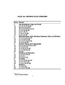


![arXiv:1011.6338v2 [math-ph] 10 Dec 2010 - IUPUI Math](https://m.moam.info/img/260x300/arxiv10116338v2-math-ph-10-dec-2010-iupui-math_5c50468c097c474a178b456e.jpg)


