Stage duration distributions in matrix population ... - Wiley Online Library
Recommend Documents
Oct 15, 2004 - Further evidence of microorganism ac- ..... Suppose there exists a hypothesis, H, pro- ...... let the 75 PCA vectors derived from our elemental .... Washington, D. C. ... (2000), Investigation of microorganisms and DNA from rock.
Temperature responses of life-history traits and per capita growth rates in a constant .... Fenchel, T. (1974) Intrinsic rate of natural increase: the relationship with.
Elizabeth E. Crone,1* Eric S. Menges,2 Martha. M. Ellis,1 Timothy Bell,3 Paulette Bierzychudek,4. Johan EhrlÃn,5 Thomas N. Kaye,6 Tiffany M. Knight,7 Peter ...
Articles. Teaching the Extracellular Matrix and Introducing Online Databases. Within a Multidisciplinary Course with i-cell-MATRIX. A STUDENT-CENTERED ...... els, 2nd ed., Berrett-Koehler, San Francisco, CA. [26] D. Stead (2005) A review of ...
Abstract. Aim: To investigate the relationship between breastfeeding and infant health and to describe growth in the first 9 months. Methods: Mothers delivering a ...
Oct 26, 2017 - two pieces of information can be used for determining the status of a threatened species. .... When the duration is short, stage structure is often embedded within age .... Ï, age; l, length; µ, number of births per adult; g, number
Jan 24, 2006 - assumed that ln Kd is negatively correlated to ln k [Burr et al., 1994 ..... The Henry's Law constant (H) is calculated for the estimated average ...
Dec 21, 2016 - Correspondence. Susan K. Skagen, U.S. Geological Survey, Fort .... areas, respectively, which also report to single point locations, we as- sumed a ...... ation of conservation strategies in southwest playa wetlands: Final report.
Jan 24, 2006 - al., 1986b; Roberts et al., 1986] is one of a few well- ... transport behaviors [Roberts et al., 1986]: (1) the solute ..... A c2 test with William's.
Jul 19, 2013 - levels were increased whereas TIMP-3 levels were similar to Lewis controls. Administration ...... I. G. Joshua, and S. C. Tyagi. 2008. Congenic ...
Nov 29, 2011 - tips. Bundles of fibronectin and tenas- cin also extend along the myocytes of the myotome ..... the tips of elongated myocytes. (Bajanca et al. .... occupied by it is free of fibronectin. (Fig. .... et al., 1999; Bajanca et al., 2006;
Feb 13, 2013 - As a result of reduced hard callus turnover, bone formation was reduced with antiresorptive ... impeded during late fracture repair in the presence of both a ...... endothelial cells and TRAPâpositive cells can collaborate to drive.
May 18, 2016 - Research Fund (MRF) of Memorial University. (funds to SS ... VEGF and MMP SNPs and Outcome in Colorectal Cancer ...... Kong, S. Y., J. W. Park, J. A. Lee, J. E. Park, .... Boyle, A. P., E. L. Hong, M. Hariharan, Y. Cheng, M.
Ikramuddin Aukhil,â Clay Walker,â¡ and Luciana Macchion Shaddoxâ . Background: Matrix metalloproteinases (MMPs) are a family of host-derived proteinases ...
Mar 5, 2013 - Jae Seok Seo,1 Jong-Ho Kim,2 Seung Woo Han,1 In San Kim,3 and Young Mo Kang1. Objective. ... domain of ÃIG-H3 was weakly effective in suppressing ..... interest function of Analysis Workstation software (Advanced.
ABSTRACT: Following retrograde menstruation, shed endometrial tissue frag- ments attach to and invade the peritoneal surface to form established endo-.
Mar 5, 2013 - Jae Seok Seo,1 Jong-Ho Kim,2 Seung Woo Han,1 In San Kim,3 and Young Mo ..... interest function of Analysis Workstation software (Advanced.
ABSTRACT: The assessment of cartilage repair has largely been limited to macroscopic observation, magnetic ..... dylar lesion treatments demonstrated a high degree of variability ..... colleagues29 suggested that tissue-engineered car-.
Webber. R. and Mumford, R.A.. (1995) Quantification of a matrix metalloproteinase-generated aggrecan GI fragment using monospecific antipeptide serum.
*Correspondence: [email protected]. Author Contribution Statement: SMP led the ..... C. M. Preston, and D. M. Karl. 2003. Abundance and dis- tribution of ...
the decadal scale to calculate the solar energy received at the surface using the sunshine duration. The dependence of sunshine duration on altitude is strong ...
Nov 27, 2001 - capecitabine metabolites in colorectal cancer patients ... respectively. Systemic exposure based on plasma concentrations of capecitabine and.
POPGENREPORT is a new R package that simplifies performing population genetics analyses ... stand-alone statistical programs for the analysis of these data.
Oct 24, 2007 - Andrew J. McLachlan1,5 ... Professor Andrew J. McLachlan, Faculty of ..... 16 Louvet C, Labianca R, Hammel P, Lledo G, Zampino MG,. Andre T ...
Stage duration distributions in matrix population ... - Wiley Online Library
May 21, 2018 - matrix models can identify key demographic parameters that influ- ... Ecology and Evolution published by John Wiley & Sons Ltd. Department of ...
|
|
Received: 1 February 2018 Revised: 18 May 2018 Accepted: 21 May 2018 DOI: 10.1002/ece3.4279
ORIGINAL RESEARCH
Stage duration distributions in matrix population models Toshinori Okuyama Department of Entomology, National Taiwan University, Taipei, Taiwan Correspondence Toshinori Okuyama, Department of Entomology, National Taiwan University, Taipei 106, Taiwan. Email: [email protected] Funding information Ministry of Science and Technology of Taiwan, Grant/Award Number: 105-2311-B-002-019-MY3
Abstract Matrix population models are a standard tool for studying stage-structured populations, but they are not flexible in describing stage duration distributions. This study describes a method for modeling various such distributions in matrix models. The method uses a mixture of two negative binomial distributions (parametrized using a maximum likelihood method) to approximate a target (true) distribution. To examine the performance of the method, populations consisting of two life stages (juvenile and adult) were considered. The juvenile duration distribution followed a gamma distribution, lognormal distribution, or zero-truncated (over-dispersed) Poisson distribution, each of which represents a target distribution to be approximated by a mixture distribution. The true population growth rate based on a target distribution was obtained using an individual-based model, and the extent to which matrix models can approximate the target dynamics was examined. The results show that the method generally works well for the examined target distributions, but is prone to biased predictions under some conditions. In addition, the method works uniformly better than an existing method whose performance was also examined for comparison. Other details regarding parameter estimation and model development are also discussed. KEYWORDS
individual variation, maximum likelihood, mixture distributions, stage duration, stagestructured models
1 | I NTRO D U C TI O N
to misleading predictions of population growth. Matrix population
The growth rate of a population is determined by the survival and
models that account for variation in demographic rates among life
reproduction of its individuals. To understand how individual-level
stages (Caswell, 2001). By explicitly considering distinct life stages,
demographic processes translate to population growth, varia-
matrix models can identify key demographic parameters that influ-
tion in demographic rates among individuals must be considered.
ence population growth, which is highly valuable in applied fields
Although trivial, only reproductively mature individuals contribute
and others (e.g., Crouse et al., 1987; Parker, 2000; Shyu & Caswell,
directly to immediate population growth. Survival rates also vary
2016). To establish the relationship between population growth and
by life stages (Pinder, Wiener, & Smith, 1978). For example, in the
demographic parameters, proper identification and characterization
loggerhead sea turtle Caretta caretta, the annual survival rate varies
of life stages are essential.
models are one of the commonly used tools to build stage-structured
among life stages: eggs, juveniles, and adults (Crouse, Crowder, &
Unless a stage is defined by a fixed duration (e.g., age), stage du-
Caswell, 1987). Ignoring the stage structure of a population can lead
ration will vary among individuals within the stage. For example, in
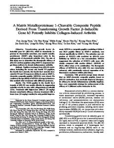
2009). In the example shown in Figure 1c, there are two indepen-
1975). The distribution of stage duration is another important detail
dent negative binomial distributions describing the duration of the
that affects population growth (de Valpine, Scranton, Knape, Ram, &
juvenile stage, and each juvenile follows one of the two distributions
Mills, 2014). However, in matrix models, it is uncommon to explicitly
for which the probabilities that a newborn enters the first and sec-
think of a probability distribution and instead use a method that cap-
ond negative binomial distributions are p and 1 − p, respectively.
tures some components (e.g., mean and variance) of a distribution.
Each negative binomial distribution is characterized by two param-
One difficulty in building matrix models is that even when we know
eters (k1,γ1) and (k2,γ2). Having five parameters (p, k1, γ1, k2, and γ2
the true distribution of stage duration, incorporating the distribu-
), mixtures of negative binomial distributions are the most flexible
tion precisely might not be possible. Although matrix models can
among the distributions described here. In fact, the geometric dis-
describe accurate dynamics when within-stage age distributions are
tribution is a special case of the negative binomial distribution (i.e.,
stable (Caswell, 2001), this assumption is not necessarily satisfied
k = 1) and the negative binomial distribution is a special case of the
(Runge & Roff, 2000). More importantly, the effects of the distribu-
mixture distribution (i.e., p = 1 or p = 0). In this study, mixtures of two
tions on population growth rate cannot be examined when specific
negative binomial distributions are referred to as a mixture distribu-
distributions of interest cannot be expressed.
tion unless otherwise stated.
To illustrate the difficulty in modeling stage duration, a species
Although a mixture distribution is more flexible than geometric
consisting of two stages (juvenile and adult) is considered in which
and negative binomial distributions, actual distributions of stage
we are interested in modeling the distribution of juvenile duration. A standard method for describing stage duration assumes that a juvenile either leaves the juvenile stage (i.e., becomes an adult) with
(a)
probability γ or remains as a juvenile with probability 1 − γ for a
100% of newborn start from this stage
Juvenile
given time step if it survives (Figure 1a). In other words, the stage
Adult
transition (per time step) is a Bernoulli process with success probability γ, with the stage duration of a juvenile realized by the number of Bernoulli trials required to have one success, which is known as a geometric distribution. A geometric distribution might be appro-
1−
1
Juvenile
(b) 100% of newborn start from this stage
priate in some cases, but is highly restrictive. For example, the expected duration of juvenile stage in the whitefly Bemisia argentifolii
Adult
is similar when they are raised on eggplant (17.31 days) and on tomato (17.96 days), but the associated variances are different: 44.47 on eggplant and 77.00 on tomato (Tsai & Wang, 1996). A geometric which suggests that it is inappropriate for both cases. Furthermore, as shown in the example, distributions can have the same mean while having different variances. Geometric distributions cannot
1−
1−
distribution whose mean is 17.5 must have its variance as 288.75,
1−
1
Juvenile
(c) Frac on p of newborn start from this stage
have different variances when they have the same mean. As such,
1
cases in which the use of a geometric distribution is appropriate 1
are limited. Extensions of the geometric distribution are used to describe stage duration more flexibly. A natural extension is the sum of geometric distributions known as the negative binomial distribution
1−
1−
1
1
Adult
Frac on 1−p of newborn start from this stage
(Caswell, 2001). A negative binomial distribution can be interpreted
2
2
2
as the number of Bernoulli trials required to have k successes.
1
Figure 1b shows an example with k = 3. To become an adult, a newly born juvenile must go through identical Bernoulli trials until three
1−
2
1−
2
1−
2
successes are achieved. In this example, the juvenile stage contains three stages known as pseudostages. Pseudostages are created for convenience (e.g., simply to make k > 1) and typically do not represent biologically meaningful stages such as age. Ages are implicit in the models considered in this study, but matrix models that consider both age and stage explicitly have also been developed (Caswell, 2012; Roth & Caswell, 2016, 2018).
F I G U R E 1 Diagrams describing stage transitions given that individuals survive. Juvenile duration follows a (a) geometric distribution, (b) negative binomial distribution, and (c) mixture of two negative binomial distributions. Each arrow indicates an event, and the associated value (e.g., γ) is the probability that the event takes place given that an individual survives
|
3
OKUYAMA
duration might differ significantly from it. Therefore, it is important to know how well a mixture distribution can approximate other potential duration distributions. A previous study found that a mixture distribution cannot approximate common distributions such as gamma and lognormal distributions effectively when the parameters of the mixture distribution are estimated heuristically (Lee & Okuyama, 2017). However, the fact that a mixture distri-
⎛ P1 ⎜ ⎜ G1 ⎜ 0 A=⎜ ⎜ 0 ⎜ ⎜ 0 ⎜ ⎝ 0
pG1 b
0
0
pG2 m
P1
0
0
0
(1 − p)G1 m
P2
0
(1 − p)G2 m
0
G2
P2
0
0
0
G2
P2
G1
0
0
G2
⎞ ⎟ ⎟ (1 − p)σA m ⎟ ⎟ ⎟ 0 ⎟ 0 ⎟ ⎟ σA ⎠ pσA m 0
(2)
bution does not perform well with heuristic parameter estimation
where Pi = σJ (1 − γi ) is the probability that a juvenile survives and
(described in Appendix) does not necessarily indicate the failure
remains in the same pseudostage, with i ∈ {1,2} representing one
of the mixture distribution when the parameters are estimated
of the two negative binomial distributions. Gi = σJ γi is the proba-
differently. The heuristic method is similar to the method of mo-
bility that a juvenile in a pseudostage survives and advances to the
ments, which uses only information contained in moments (e.g.,
next stage (another pseudostage or the adult stage). The model
the mean and variance), and it might make little sense when the
assumes that the stage duration TJ is a latent trait (i.e., determined
assumed distribution is known to be wrong (e.g., using a mixture
at the birth), and an observed distribution can significantly differ
distribution to approximate a gamma distribution), and when infor-
from the distribution of TJ because some individuals die before be-
mation not contained in moments influences population dynam-
coming adults (further discussed below, also see Ergon, Yoccoz, &
ics. Maximum-likelihood estimation accounts for other properties
Nichols, 2009). The distribution of latent stage duration coincides
of distributions through a fuller utilization of data (e.g., not just
with the observed distribution only when all individuals survive till
the mean and variance). This study examined the performance
adults (i.e., σJ = 1).
of a mixture distribution in approximating other target distributions when model parameters were estimated using a maximum- likelihood method.
2.2 | Model parameters and analysis Maximum-likelihood estimates (MLEs) of (p, k1, γ1, k2, and γ2) were used to create matrix models. When f is the true distribution of
2 | M E TH O DS
stage durations (i.e., TJ ~ f), a matrix model uses a mixture distribution to approximate f. For a given true (or target) distribution of juvenile duration f (specific distributions will be described below),
2.1 | Matrix population model
the maximum-likelihood parameters of a mixture distribution were
A species that experiences two life stages, such as the one shown
estimated from 1,000 random samples generated from f.
in Figure 1, is considered. The matrix model uses a postbreeding
Once the MLEs are determined, a population matrix (e.g.,
census formulation (Case, 2000; Caswell, 2001) to keep track of
Equation 2) can be fully specified with the three additional parame-
the number of individuals in each stage and assumes that the dura-
ters σJ, σA, and m. Specific parameter values are discussed below. In
tion of juvenile stage TJ follows a mixture distribution. For exam-
this study, A is an irreducible primitive matrix that makes the popu-
ple, Figure 1c describes the stage transitions when k1 = 2 and k2 = 3.
lation ergodic according to the Perron-Frobenius theorem (Caswell,
Additional parameters describing survival and reproduction must be
2001). In other words, the population growth rate eventually con-
specified to complete a full demographic model. σJ and σA are the
verges to a fixed value regardless for any positive initial condition,
survival probabilities for juvenile and adult, respectively, and m is the
and the asymptotic population growth rate (i.e., the finite rate of in-
expected number of female offspring produced by an adult female.
crease) is represented by the dominant eigenvalue of A. In one sim-
All parameters describe demographic processes that take place in
ulation run, random samples from f are used to parametrize A, and
one discrete time step (e.g., day, week, or year), and an appropriate
the finite rate of increase is estimated from A. Because the finite rate
time step should depend on organisms (Cull, 1980). The model as-
of increase fluctuates as a result of random sampling from f, the av-
sumes that males do not limit reproduction and keeps track only of
erage from 100 simulation runs was used to represent the expected
females (Caswell, 2001).
value of the finite rate of increase.
Matrix population models can be described as N(t + 1) = AN(t)
(1)
2.3 | Individual-based models (IBMs) The matrix model described above assumes that juvenile duration
where N(t) is a vector that consists of the number of individuals in
follows a mixture distribution. When the true distribution, f, is not a
each stage at time t. For example, for Figure 1c, N(t) is a vector length
mixture distribution, the matrix model is an approximation. Examining
of six (i.e., five pseudostages and one adult stage). A completely sum-
the performance of matrix models when f is not a mixture distribu-
marizes the demographic processes. Using the postbreeding census
tion requires knowing the true population growth under f. An IBM
method, a mixture distribution- based model corresponding with
was created to obtain population growth for various instances of f.
Figure 1c is,
Because matrix models describe simple demographic processes that
|
OKUYAMA
4
occur in discrete time steps, corresponding IBMs can be created by
Negative binomial distributions can be defined in multiple man-
simulating the demographic processes. For example, the survival of
ners. One form of negative binomial distribution was already de-
individuals is simulated as a Bernoulli trial with the survival probabili-
scribed above (e.g., Figure 1b; also see Appendix). Another formulation
ties σJ (for juveniles) and σA (for adults). For each newly born individual,
uses two parameters μ and k, where the mean is μ and the variance is
the duration of its juvenile stage is simulated from f. If the stage dura-
μ + μ2/k (Bolker, 2008). This form of negative binomial distributions is
tion of a juvenile is x, the juvenile becomes an adult if it survives x time
referred as over-dispersed Poisson distributions in this study to avoid
steps. Each adult reproduces m offspring on average, and the number
confusion between the two negative binomial distributions.
of offspring was simulated from a Poisson distribution with mean m.
For gamma and lognormal distributions, random samples were
The finite rate of increase of a population can be estimated by
rounded up to the nearest integer (i.e. ceiling). Taking the ceiling
simulating the IBM for many time steps. In particular, N(t + 1)/N(t)
eliminates zero and results in discrete random samples. Because ma-
converges to the finite rate of increase, where N(t) is the number of
trix models are discrete time models, the realized stage durations
individuals at time t (the sum of all individuals at time t). N(t + 1)/N(t)
must be discrete. As discussed above, a previous study found that
will fluctuate some even after convergence as a result of the sto-
mixture distributions (based on the heuristic method) fail to approx-
chastic nature of the model. The geometric mean of N(t + 1)/N(t)
imate gamma and lognormal distributions, and thus, these distribu-
from the last 1,000 time steps of 2,000 total time steps was used to
tions present good tests for the current study. Furthermore, these
represent the finite rate of increase. It was confirmed that a burn-in
distributions are among the most commonly used distributions for
period of 1,000 was sufficient to obtain convergence.
describing nonnegative random variables. To examine the performance a mixture model in approximating f (i.e., TJ ~ f), the mean and variance of f were varied systematically
2.4 | Comparison of the matrix model and IBM results
when possible. To obtain a target distribution with specified mean E(TJ) and variance Var(TJ), the method of moment estimates was used
Estimates of the finite rate of increase from the matrix model and
(e.g., the shape and scale parameters of a gamma distribution, re-
the IBM were compared under various choices of f in TJ ~ f. The IBM
spectively, are E(TJ)2/Var(TJ) and Var(TJ)/E(TJ)). For gamma and log-
describes true (target) dynamics, and thus, a difference in prediction
normal distributions, E(TJ) and Var(TJ) are the mean and variance
between an IBM and the corresponding matrix model indicates an
without the ceiling, and thus, the actual mean and variance differ
inaccuracy in the matrix model. Four parametric distributions were
slightly from E(TJ) and Var(TJ). For zero- truncated Poisson distri-
considered for f: (a) zero-truncated Poisson distributions, (b) zero-
butions, only the mean was set to a desired value. Zero-truncated
Poisson distributions have one parameter λ with E(TJ) = λ∕(1 − e−λ ),
(discrete) gamma distributions, and (d) (discrete) lognormal distribu-
and Var(TJ) = E(TJ)(1 + λ − E(TJ)). Therefore, setting the expected du-
tions. The zero-truncated distributions were used because a juvenile
ration E(TJ) automatically determines the associated variance.
duration of zero indicates that adults are directly producing adults, which was assumed to be impossible in this study.
For this study, producing meaningful comparisons requires that the IBM and the matrix model must be defined consistently. In other
E(TJ) = 3
E(TJ) = 19
E(TJ) = 35
Finite rate of increase
1.25 1.125
4
model
1.20
IBM
1.100 3
likelihood 1.15
heuristic 1.075
2 1.10 1.050 0.5
1.0
1.5
2.0
0.5
1.0
1.5
2.0
0.5
1.0
1.5
2.0
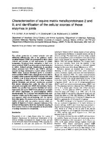
Var(TJ) E(TJ) F I G U R E 2 Relationship between the distribution of juvenile duration and the finite rate of increase. The true distribution used in the IBM is a mixture distribution whose parameters were determined using the heuristic method. E(TJ) and Var(TJ) were systematically varied. For example, when Var(TJ)/E(TJ) = 2 and E(TJ) = 3, Var(TJ) = 6. In each E(TJ) figure, it appears that there are three lines corresponding with sJ = 0.95 E(T ) (top line), sJ = 0.5 (middle line), and sJ = 0.05 (bottom line) where σJ J = sJ, but each of the three lines consists of three additional overlapping lines, because the three models show identical results. σA = 0.95, m = 10
|
5
OKUYAMA
words, if a mixture distribution is used as f in an IBM, then the IBM
is approximately three at 25°C. To reflect this, the average juvenile
and the corresponding matrix model must produce the same finite
duration E(TJ) was varied from three to 35 days in this study, and the
rate of increase. This check is shown in Results. In addition, the per-
ratio of variance to mean Var(TJ)/E(TJ) was varied from 0.1 to 2.0. The
formance of matrix models with the heuristic method is also included
probability that a newly born juvenile survives to become an adult
as a reference. For convenience, matrix models parametrized by the
sJ was varied from 0.05 to 0.95 to consider as nearly full a param-
heuristic and likelihood methods, respectively, are referred to as the
eter range as possible. The daily juvenile survival probability σJ was
heuristic and likelihood models.
computed from the relationship, σJ
E(TJ )
Parameters associated with a true scenario are the parameters of
= sJ. The daily adult survival
probability σA was varied from 0.5 to 0.98, corresponding to the aver-
f (e.g., mean and variance of juvenile duration), σJ, σA, and m. Because
age adult duration (i.e., adult longevity) from two to 50 days, whereas
the theoretically possible parameter space is infinitely large, a specific
an adult B. dorsalis survives approximately 40 days under laboratory
parameter space must be specified. Parameter values were informed
conditions. The median of daily fecundity is approximately 15 eggs.
from the life cycle of the oriental fruit fly (Bactrocera dorsalis) (Fang
Assuming a 1:1 sex ratio, the number of female eggs is approximately
et al., 2011). The matrix A in Equation 1 describes demographic pro-
seven. To reflect this, m was varied from five to 15. Thus, the param-
cesses that take place in one day. The sum of the average durations of
eter space was set liberally to reflect a much greater parameter space
juvenile stages is approximately 30 days, and the associated variance
than might be realized by B. dorsalis. Furthermore, as will be explained
σ A = 0.5, s J = 0.05
σ A = 0.5, s J = 0.5
1.6
7
σ A = 0.5, s J = 0.95
6
4
5 1.4
3
1.2
4 3
2
2 2.5
5.0
7.5
Finite rate of increase
σ A = 0.95, s J = 0.05
10.0
2.5
5.0
7.5
σ A = 0.95, s J = 0.5
10.0
2.5
5.0
7.5
σ A = 0.95, s J = 0.95
10.0
5 2.0 6
4
1.8
model IBM
1.6
3
likelihood
4
heuristic 1.4
2
2
1.2 2.5 2.2
5.0
7.5
σ A = 0.98, s J = 0.05
10.0
2.5
5.0
7.5
σ A = 0.98, s J = 0.5
10.0
2.5
5.0
7.5
10.0
2.5
5.0
7.5
10.0
σ A = 0.98, s J = 0.95
5
2.0
6
4
1.8
3
1.6 1.4
4
2
2
1.2 2.5
5.0
7.5
10.0
2.5
5.0
7.5
10.0
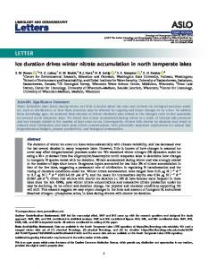
E(TJ) F I G U R E 3 Relationship between the distribution of juvenile duration and the finite rate of increase. The true distribution used in the IBM is a zero-truncated Poisson distribution with mean E(TJ). m = 10
|
OKUYAMA
6
below, although σJ, σA, and m influence the finite rate of increase, they
f, indicating that the parameter estimation methods performed
do not qualitatively influence how the distribution of duration influ-
sufficiently well.
ences the finite rate of increase. Therefore, the survival and fecundity
Both the heuristic and likelihood models performed gener-
parameters are not crucial factors in this study. The source code in R
ally well when f is a zero-truncated Poisson distribution (Figure 3).
used in the analysis is provided as Supporting Information.
Figure 3 focuses on short juvenile durations (E(TJ) ≤ 10), because the difference among the models becomes smaller as E(TJ) becomes longer, as can also be inferred from the figure. When E(TJ) is greater than
3 | R E S U LT S
3 days, the likelihood model overestimates population growth rates, whereas the heuristic model underestimates them.
When the distribution of juvenile duration in an IBM, f, is a mix-
Among offspring that are born at the same time, those with short
ture distribution whose parameters are determined by the heu-
juvenile durations contribute to the population growth dispropor-
ristic method (Appendix), the IBM and matrix models result in
tionately more than those with longer juvenile durations. For exam-
identical population growth rates for all parameter combinations
ple, if we compare a juvenile with a duration of 1 day and another
(Figure 2), showing that the IBM and the matrix models are de-
with a duration of 5 days, the former juvenile will start producing
fined consistently such that comparisons based on other distribu-
offspring at the next breeding event, and there will already be grand-
tions of f are meaningful. In addition, the parameters of mixture
children in the following time step even when the latter individual
distributions in the matrix models were estimated from random
is still juvenile. Consequently, producing two offspring whose juve-
samples of f rather than through using the known parameters of
nile durations are 1 and 5 days, respectively, can result in a greater
E(TJ) = 3
E(TJ) = 5
E(TJ) = 7
4.0
1.9
2.4 3.8
2.3
3.6
1.8
2.2 2.1
3.4
1.7
2.0 3.2
Finite rate of increase
E(TJ) = 9
1.6
E(TJ) = 11
1.48
E(TJ) = 13
1.38
1.60 1.36
1.44
model IBM
1.55 1.34
likelihood heuristic
1.40
1.50
1.32
1.45
1.36
E(TJ) = 15
E(TJ) = 17
1.27
E(TJ) = 19
1.31 1.23
1.26
1.30 1.29
1.25
1.22
1.28 1.24 1.27
1.21 1.25
1.50
1.75
2.00
1.25
1.50
1.75
2.00
1.25
1.50
1.75
2.00
Var(TJ) E(TJ) F I G U R E 4 Relationship between the distribution of juvenile duration and the finite rate of increase. The true distribution used in the IBM is a zero-truncated over-dispersed Poisson distribution with mean E(TJ) and variance Var(TJ). m = 10, σA = 0.95, sJ = 0.5
|
7
OKUYAMA
population growth rate than producing two offspring whose juvenile
likelihood model performs relatively poorly when E(TJ) takes on
durations are both 3 days, even though the average juvenile duration
some intermediate values, but when E(TJ) is very low or high, the
is the same for both cases when not considering survival. This is a
bias becomes negligible. On the other hand, estimates from the
positive effect of Var(TJ). Depending on the strength of the positive
heuristic model are significantly lower than the true values regard-
effect of Var(TJ) and the negative effect of E(TJ), the relationship be-
less of E(TJ).
tween the population growth rate and E(TJ) is not monotonic (e.g.,
For a given combination of mean and variance, the gamma distri-
when sJ = 0.05 and E(TJ) 1.1 are
E(TJ) ≥ 13, the qualitative relationship between Var(TJ)/E(TJ) and the
shown because the variance of an over-dispersed Poisson distri-
finite rate of increase does not change (i.e., the proportional biases
bution must be greater than its mean. For a given mean duration
do not change), even though the finite rate of increase decreases as
E(TJ), the variance does not have a strong effect on the bias, but
E(TJ) increases. For this reason, results from E(TJ) > 19 are not shown
the mean duration strongly influences the bias. For example, the
in Figure 5.
E(TJ) = 3
E(TJ) = 5
E(TJ) = 7
4.0 2.2
3.5
1.7
2.0
3.0 2.5
1.8
2.0
1.6
1.6
1.5
Finite rate of increase
E(TJ) = 9
E(TJ) = 11 1.40
1.50
1.45
E(TJ) = 13
1.350
model IBM
1.325
likelihood heuristic
1.36
1.300
1.32
1.275
distribution
1.40
gamma lognormal
1.35
E(TJ) = 15
1.250
E(TJ) = 17
1.26
E(TJ) = 19
1.23 1.22
1.28 1.24
1.21 1.26 1.20
1.22 1.24
1.19 1.20 0.5
1.0
1.5
2.0
0.5
1.0
1.5
Var(TJ) E(TJ)
2.0
1.18
0.5
1.0
1.5
2.0
F I G U R E 5 Relationship between the distribution of juvenile durations and the finite rate of increase. The true juvenile durations are the ceilings of numbers from a gamma or lognormal distribution with mean E(TJ) and variance Var(TJ). m = 10, σA = 0.95, sJ = 0.5
|
OKUYAMA
8
The other parameters (i.e., s J , σA, and m) positively influence
track other properties of a distribution and reasonably approxi-
the finite rate of increase, but they do not qualitatively affect
mates population growth rates under commonly used distributions,
the relationship between Var(TJ )/E(TJ ) and the finite rate of in-
such as lognormal, gamma, and zero- truncated (over- dispersed)
crease. To illustrate this point, the effect of s J (where σJ
Poisson distributions.
E(TJ )
= sJ) is
shown in Figure 6. For a given E(TJ ), changing s J from 0.05 to 0.95
It should be noted that the distribution of stage durations is
has little influence on the relationship other than that population
defined for all individuals including those that do not reach the
growth rates generally increase with s J . The same is true for σA
next stage. Suppose that T (the subscript J is omitted to indicate
and m.
an arbitrary stage) follows a gamma distribution. Observed stage durations based on surviving individuals do not follow the gamma distribution unless the mortality (1-σ) is negligible. In other words,
4 | D I S CU S S I O N
when Q is the stage duration of individuals that survive to the next stage, Q = T only when σ = 1. Because in a study, we only have
Stage- specific characteristics, such as the distribution of stage
data from Q, the effect of mortality on stage durations must be ex-
durations, influence the growth rate of a stage-s tructured popula-
plicitly incorporated into the parameter estimation procedure. The
tion. Because a probability distribution cannot be described fully
probability that an individual survives x time steps and reaches the
in terms of its mean and variance, a heuristic model that depends
next stage is
solely on the mean and variance of a distribution will likely produce
E(TJ) = 3, sJ = 0.05
(3)
Prob(Q = x) = g(x)σx
misleading conclusions. On the other hand, a likelihood model can
E(TJ) = 3, sJ = 0.5
E(TJ) = 3, sJ = 0.95
4.0 2.1
3.5
1.8
3.0
1.5
2.5
1.2
2.0
Finite rate of increase
E(TJ) = 5, sJ = 0.05
4
3
E(TJ) = 5, sJ = 0.5
2.6
E(TJ) = 5, sJ = 0.95 model
2.2
1.6
IBM
2.4
likelihood 2.0
2.2
1.8
2.0
heuristic
1.4
1.2
gamma lognormal
1.8
1.6
E(TJ) = 7, sJ = 0.05
distribution
E(TJ) = 7, sJ = 0.5
1.9
1.4 1.7
E(TJ) = 7, sJ = 0.95
1.8
1.3 1.6
1.2
1.7
1.5
0.5
1.0
1.5
2.0
1.6
0.5
1.0
1.5
Var(TJ) E(TJ)
2.0
0.5
1.0
1.5
2.0
F I G U R E 6 Relationship between the distribution of juvenile durations and the finite rate of increase. The true juvenile durations are the ceilings of numbers from a gamma or lognormal distribution with mean E(TJ) and variance Var(TJ). m = 10 and σA = 0.95
|
9
OKUYAMA
where g is the probability mass function (e.g., a mixture of two nega-
is very restrictive as discussed above, the sum of a constant and a
tive binomial distributions) that is used in a matrix model. Supposing
geometric distribution is more flexible and can be expressed in ma-
that there are N individuals initially, and that S individuals survive to
trix models. Although it is currently customary to report only the
the next stage, this process can be described as
mean and variance of data, more detailed examination of stage du-
S ∼ Binomial(N,
∑∞
x=1
g(x)σx )
ration would assist us in identifying important properties of duration (4)
where the second argument of the binomial distribution is the prob-
distributions beyond the mean and variance, as well as appropriate models for approximating target distributions in matrix models.
ability parameter that describes the probability that an individual survives the focal stage. The maximum- likelihood parameters of both g and σ can be obtained from these relationships. Ergon et al.
AC K N OW L E D G M E N T S
(2009) provide a method for estimating the latent distribution T from
I thank Dr. Torbjørn Ergon and anonymous reviewers for insightful
capture–recapture data. When a matrix model is defined based on
comments. This study was supported by the Ministry of Science and
a latent distribution (e.g., Equation 2), the estimation of the latent
Technology of Taiwan (Grant ID: 105-2311-B-0 02-019-MY3).
distribution is essential. Relatively poor performance of the likelihood model when E(TJ) is short is a valid concern, because none of the parametric distributions considered in this study is unrealistic. Although this study
C O N FL I C T O F I N T E R E S T None declared.
combined all sexually immature stages (e.g., egg and larva stages) into one stage, stage-structured models may consider these stages explicitly (e.g., Bommarco, 2001; Lončarić & Hackenberger, 2013), making the duration of each stage short. Even when there are no
AU T H O R C O N T R I B U T I O N TO performed all work presented in this study.
distinct life stages such as larval and pupal stages, size-dependent mortality is commonly reported (e.g., Grutter et al., 2017; Remmel & Tammaru, 2009). To capture size-dependent mortality rates, a stage
DATA AC C E S S I B I L I T Y
(e.g., juvenile stage) may be further subdivided into size classes (e.g.,
The computer code in R used in the analysis is available in Supporting
Crouse, Crowder, & Caswell, 1987), which also makes the duration of
Information.
each class short. One way to improve approximation is to extend the mixture distribution. For example, mixtures of more than two distributions can be considered. It is useful to recognize that when there are n distinct stage durations (e.g., n = 4 when observed durations
ORCID Toshinori Okuyama
http://orcid.org/0000-0002-9893-4797
are always between 5 and 8 days), a multinomial distribution with probability parameters matching the proportions of observed durations can be considered a full model. Because a multinomial distribution with n possible outcomes can be expressed as a mixture of n constants (e.g., Figure 1c describes a binomial distribution with two possible outcomes (i.e., two or three) when γ1 = γ2 = 1), mixtures of sufficiently many distributions will describe any observed data accurately. One can conduct model selection against the full model to determine the complexity of the required model. When modeling a distribution, using a commonly used model (including the mixture distribution) for convenience might not be well advised. A distribution can be customized when information regarding it is available (e.g., the multinomial distributions discussed above). For example, there may be a minimal duration required for some stages (e.g., Dzierzbicka-Głowacka, 2004; Oyarzun & Strathmann, 2011). If a model predicts some individuals stay only 2 days in a stage although at least 3 days are needed to develop into the next stage due to some biological constraints, this inaccuracy can be a cause of important mismatch between model predictions and observations. In a situation like this, adding a constant can assure the required duration in the stage and may describe the target distribution reasonably well. For example, even though the geometric distribution
REFERENCES Birt, A., Feldman, R. M., Cairns, D. M., Coulson, R. N., Tchakerian, M., Xi, W. M., & Guldin, J. M. (2009). Stage-structured matrix models for organisms with non-geometric development times. Ecology, 90, 57–68. https://doi.org/10.1890/08-0757.1 Bolker, B. (2008). Ecological models and data in R. Princeton, NJ: Princeton University Press. Bommarco, R. (2001). Using matrix models to explore the influence of temperature on population growth of arthropod pests. Agricultural and Forest Entomology, 3, 275–283. https://doi. org/10.1046/j.1461-9555.2001.00114.x Case, T. J. (2000). An illustrated guide to theoretical ecology. Oxford, UK: Oxford University Press. Caswell, H. (2001). Matrix population models: Construction, analysis, and interpretation. Sunderland, MA: Sinauer Associates. Caswell, H. (2012). Matrix models and sensitivity analysis of populations classified by age and stage: A vec- permutation matrix approach. Theoretical Ecology, 5, 403–417. https://doi.org/10.1007/ s12080-011-0132-2 Crouse, D. T., Crowder, L. B., & Caswell, H. (1987). A stage-based population model for loggerhead sea turtles and implications for conservation. Ecology, 68, 1412–1423. https://doi.org/10.2307/1939225 Cull, P. (1980). The problem of time unit in Leslie’s population model. Bulletin of Mathematical Biology, 42, 719–728.
|
OKUYAMA
10
Dzierzbicka-Głowacka, L. (2004). Growth and development of copepodite stages of Pseudocalanus spp. Journal of Plankton Research, 26, 49–60. https://doi.org/10.1093/plankt/fbh002 Ergon, T., Yoccoz, N. G., & Nichols, J. D. (2009). Estimating latent time of maturation and survival costs of reproduction in continuous time from capture-recapture data. In D. Thomson, E. G. Cooch & M. J. Conroy (Eds.), Modeling demographic processes in marked populations (pp. 173–197). Boston, MA: Springer. https://doi.org/10.1007/978-0-387-78151-8 Fang, C. C., Okuyama, T., Wu, W. J., Feng, H. T., & Hsu, J. C. (2011). Fitness costs of an insecticide resistance and their population dynamical consequences in the oriental fruit fly. Journal of Economic Entomology, 104, 2039–2045. https://doi.org/10.1603/EC11200 Grutter, A. S., Blomberg, S. P., Fargher, B., Kuris, A. M., McCormick, M. I., & Warner, R. R. (2017). Size-related mortality due to gnathiid isopod micropredation correlates with settlement size in coral reef fishes. Coral Reefs, 36, 549–559. https://doi.org/10.1007/s00338-016-1537-6 King, E. G., Brewer, F. D., & Martin, D. F. (1975). Development of Diatraea saccharalis [Lep.: Pyralidae] at constant temperatures. Entomophaga, 20, 301–306. https://doi.org/10.1007/BF02371955 Lee, C. C., & Okuyama, T. (2017). Individual variation in stage duration in matrix population models: Problems and solutions. Biological Control, 110, 117–123. https://doi.org/10.1016/j.biocontrol.2017.04.011 Lončarić, Ž., & Hackenberger, B. K. (2013). Stage and age structured Aedes vexans and Culex pipiens (Diptera: Curicidae) climate-dependent matrix population model. Theoretical Population Biology, 83, 82–94. Oyarzun, F. X., & Strathmann, R. R. (2011). Plasticity of hatching and the duration of planktonic development in marine invertebrates. Integrative and Comparative Biology, 51, 81–90. https://doi.org/10.1093/icb/icr009 Parker, I. M. (2000). Invasion dynamics of Cytisus scoparisu: A matrix model approach. Ecological Applications, 10, 726–743. https://doi. org/10.1890/1051-0761(2000)010[0726:IDOCSA]2.0.CO;2 Pinder, J. E., Wiener, J. G., & Smith, M. H. (1978). The Weibull distribution: A new method of summarizing survivorship data. Ecology, 59, 175–179. https://doi.org/10.2307/1936645 Remmel, T., & Tammaru, T. (2009). Size- dependent predation risk in tree-feeding insects with different colouration strategies: A field experiment. Journal of Animal Ecology, 78, 973–980. https://doi. org/10.1111/j.1365-2656.2009.01566.x Roth, G., & Caswell, H. (2016). Hyperstate matrix models: Extending demographic state spaces to higher dimensions. Methods in Ecology and Evolution, 7, 1438–1450. https://doi.org/10.1111/2041-210X.12622 Roth, G., & Caswell, H. (2018). Occupancy time in sets of states for demographic models. Theoretical Population Biology, 120, 62–77. https:// doi.org/10.1016/j.tpb.2017.12.007 Runge, J. A., & Roff, J. C. (2000). The measurement of growth and reproductive rates. In R. Harris, P. Wiebe, J. Lenz, H. R. Skjoldal, & M. Huntley (Eds.), ICES zooplankton methodology manual (pp. 401–454). London, UK: Academic Press. https://doi.org/10.1016/B978-012327645-2/50010-4 Shyu, E., & Caswell, H. (2016). A demographic model for sex ratio evolution and the effects of sex-biased offspring costs. Ecology and Evolution, 6, 1470–1492. https://doi.org/10.1002/ece3.1902 Tsai, J. H., & Wang, K. (1996). Development and reproduction of Bemisia argentifolii (Homoptera: Aleyrodidae) on five host plants. Environmental Entomology, 25, 810–816. https://doi.org/10.1093/ee/25.4.810 de Valpine, P., Scranton, K., Knape, J., Ram, K., & Mills, N. J. (2014). The importance of individual developmental variation in stage-structured population models. Ecology Letters, 17, 1026–1038. https://doi. org/10.1111/ele.12290
S U P P O R T I N G I N FO R M AT I O N Additional supporting information may be found online in the Supporting Information section at the end of the article.
How to cite this article: Okuyama T. Stage duration distributions in matrix population models. Ecol Evol. 2018;00:1–10. https:// doi.org/10.1002/ece3.4279
APPENDIX This section describes the mixture distribution and the heuristic parameter estimation method discussed in the main text. When T is a random variable that follows a mixture distribution, (5)
T = pY1 + (1 − p)Y2
where Y1 and Y2 are random variables that follow independent negative binomial distributions such that Y1 ~ NegBin(k1,γ1) and Y2 ~ NegBin(k2,γ2) in which the probability mass function of NegBin(k,γ) is P(Y = y) =
(
y−1 k−1
)
( )y−k γk 1 − γ
(6)
that can be interpreted as the sum of k geometric distributions with parameter γ. p ∈ [0,1] is the mixture probability such that T is a single negative binomial distribution when p = 0 or p = 1. The mean and variance of the mixture distribution (Equation 5), respectively, are E(T) = pE(Y1 ) + (1 − p)E(Y2 )
(7)
Var(T) = p(E(Y1 )2 + Var(Y1 )) + (1 − p)(E(Y2 )2 + Var(Y2 )) − E(T)2 (8) where E(Yi) = ki/γi and Var(Yi) = ki (1-γi)/γ2i (i ∈ {1,2}). The heuristic method determines the parameters as follows. A mixture distribution with mean E(T) and Var(T) has k1 =
k2 =
⌊
E(T)2 Var(T) + E(T)
⌋
(9)
⌈
E(T)2 Var(T) + E(T)
⌉
(10)
where ⌊x⌋ and ⌈x⌉ are the floor and ceiling of x, respectively. The
method further assumes that γ = γ1 = γ2, leaving two remaining free parameters (p and γ) that can be determined by solving Equations 7 and 8 (i.e., two equations and two unknowns). When the data are available, E(T) and Var(T) are replaced by the sample mean and variance.