Modeling and Reasoning with Star Calculus: An Extended Abstract Debasis Mitra Department of Computer Sciences Florida Institute of Technology Melbourne, FL 32901, USA E-mail:
[email protected] 1. Introduction Spatial knowledge representation (KR) schemes are important in many areas of computation, e.g., geographical information systems, natural language technology, image processing, battlefield management, etc. In this paper we have discussed a spatial KR technique for the purpose of expressing angular relations between points in Euclidean space. The scheme is a hybrid of what are known as quantitative and qualitative schemes. In this section we will briefly introduce a related area for the purpose of motivation. Digital image processing sometimes deploys a method called “chain code” in order to represent a polygon as a sequence of angular relations between the respective pairs of points of the polygon [Gonzalez and Wintz, 1997]. The angles are measured with reference to an absolute direction in the space (e.g., North), in a clockwise or typically anti-clockwise sense. The measurement is discrete rather than continuous, i.e., they come from a finite discrete set of values between 0 and 360 degrees, e.g., {x=0°, x=30°, x=60°, . . ., x=330°}, for an angular direction x. Actually the ordering index is utilized rather than the angle’s value, e.g., {1 for x=0°, 2 for x=30°, . . ., 12 for x=330°} for the above set. Thus, a polygon will be represented as a sequence of these numbers for adjacent pairs of points on its perimeter (Figure 1). Obviously the discretization looses some information and thus, may distort the polygon when it is recovered. However, chain codeschemes may use different level of granularity, e.g., representation with 15° instead of 30°, depending on the requirement in an application.
16 20 0
Figure1: A chain-code representation with 30° angular zoning. Numbers on some of the arrowheads indicate the zones of the arrows. The Star-calculus representation scheme for reasoning with similar type of angular information, which we have invented independently [Mitra, 2002, 2002-2],
subsumes the “chain code” technique. If the chain code is termed as a quasi-quantitative knowledge representation technique, then Star-calculus is a hybrid of qualitative and quantitative representation technique. As we will see in a subsequent section, the Starcalculus generalizes over the chain code by allowing both the 1-dimensional lines and the 2-dimensional conical regions in between the semi-infinite lines. Thus, the Star-calculus is a more complete representation than the chain-code as a knowledge representation technique. A noteworthy point about our contribution is that we have extended Helly’s theorem (in linear algebra, see Chvátal, 1983). This extension may have a broader impact beyond our work on Star-calculi. 2. Spatio-temporal Qualitative Representation Revisited Starting from the early studies of simple point-based calculus in linear time, spatiotemporal constraint-based reasoning has matured into a discipline with its own agenda and methodology [Chittaro and Montanari, 2000]. The study of such a calculus starts with an underlying “space” and develops a set of jointly exhaustive and pair-wise disjoint (JEPD) “basic relations” with respect to a reference object located in that space. Basic relations correspond to some equivalent regions in the space, for the purpose of placing a second object there with respect to the first one. An equivalent region is such that the second object could be placed anywhere in this region without affecting the relation with the reference object. The underlying space and such a relative zoning scheme of the space with respect to a reference object - forms a calculus in the context of spatio-temporal knowledge representation. Qualitative reasoning with such a spatio-temporal calculus involves a given set of objects (e.g., points or time-intervals) located in the corresponding “space” and binary disjunctive relations between some of those objects. Each disjunctive binary relation is a subset of the set B of JEPD basic relations. The satisfiability question in the reasoning problem is - whether those relational constraints are consistent with respect to each other or not. The power set of B is closed with respect to the primary reasoning-operators like composition, inversion, set union and set intersection, thus, forming an algebra. Typically these algebras are Relational Algebras in the Tarskian sense [Jonsson and Tarski, 1952]. 3. The Star-calculus Star-calculus(α), where α stands for any even integer >0, involves a generalized angular zoning scheme with respect to a point in the 2D space, with (360/α)-degree angle between any consecutive pair of lines. The set B of (2*α +1) number of basic relations is {Eq, 0, 1, 2, 3, …, 2*α-1}, where ‘Eq’ is the identity relation with respect to the reference point, every even-numbered relation corresponds to a semi-infinite line fanning away from the origin, and the odd-numbered relations indicate a pie-slice or conicsectional region between two such consecutive semi-infinite lines. Figure 2 corresponds to the Star-calculus(α=12) with 30° angle between the lines. So, there are two types of basic relations in B depending on the dimensionality, other than the relation ‘Eq’ that has zero dimensionality: re of even type corresponding to a 1D-region (semi-infinite line) and ro of odd type corresponding to a 2D-region (conic-section).
0
22
2 23
1 4
20
21
3
19
5 6
eq
18 17
7 15
9
8
11 10
16
13 14 12
Figure 2: Representation of Star-calculus(12) Figure 3 shows a canonical representation G(α), indicating the topological relationship between the basic relations in the Star-calculus(α). Each circle represents an equivalent region/basic relation (synonymously used in this paper), the dark ones are the 2D-regions, the white ones are the 1D-regions, the central dot represents the Eq region, and the arcs represent the adjacency between the regions. 0 1
2α +1
2
•
Figure 3: Canonical representation G(α) of the Star-ontology(α) 4. Geometrical Modeling: Representing Polygons Qualitatively As in chain code representation, a polygon may be represented with a Star-calculus (for some integer value of α). Exhaustively, we could express all possible binary relations between every pair of points, n(n-1)/2 of them, for n points. However, we really need only n number of such binary relations between adjacent pairs of points. Example 1: A quadrilateral may be described Star-calculus(12) (i.e., θ =30°) as {(p1 2 p2), (p2 22 p3), (p3 14 p4), (p4 8 p1)}. An obvious point to note about the proposed representation scheme is that it is inaccurate from a strict quantitative point of view. This means that a polygon recovered from such a given description (e.g., example 1) may be distorted. It can be easily checked [Mitra, 2002-3] that the error of such a representation with a θ-degree angular zoning scheme is:
(1) any internal angle may be deviated by maximum 2θ in the process of recovery, and (2) the relative orientation of the whole polygon may be deviated by maximum θ. 5. Computational Complexity Issues [Definition 1] The set of all disjunctive relations, the power set P(B) of the set of the basic relations B={Eq, 0, 1, 2, 3, …, 2*α-1} is closed under disjunctive composition, inverse, set union and intersection operations, forming the Star-algebra(α). A reasoning problem instance in any subset Θ of P(B) is expressed as (V, E), where V is a set of points situated in the 2D-space, and E is a set of binary constraints Rij between some of the pairs of points i, j in V such that any Rij ∈ Θ. The satisfiability question in the reasoning problem is to check if it is feasible to assign the points in the space following all the constraints in E. Theorem 1 [Mitra, 2002-2]: Reasoning with full Star-algebra(α) is NP-complete. Proof sketch: Construction of a problem instance in the Star-algebra from an arbitrary 3SAT problem instance would be as follows. (1) For every literal lij (in the source 3-SAT problem), create two points Pij and Rij such that Pij [1 -> (α+1)] Rij, and (2) for every clause Ci we have Pi1 [(α+1) -> (2*α-1)] Ri2 and Pi2 [(α+1) -> (2*α-1)] Ri3 and Pi3 [(α+1) -> (2*α-1)] Ri1. Here, a binary relation x [r1->r2] y indicates a disjunctive set of basic relations from point x to point y, within the range from r1 through r2 over G(α). Also, (3) for every literal lij that has a complementary literal lgh we have two relations between their corresponding points: Pij [(α-1) -> (2*α-1)] Rgh and Pgh [(α-1) -> (2*α-1)] Rij. The source 3-SAT problem instance is satisfiable iff the corresponding Spatial reasoning problem instance is so, and the construction takes polynomial time with respect to the number of clauses and variables. Hence, the reasoning problem in Star-algebra(α) is NPhard. Given some binary constraints between a set of points in any Star-calculus(α), and a set of assignment for those points in the 2D-space (e.g., by their Cartesian coordinates), it could be easily verified if the assignment follows the constraints, in O(|E|) time, for |E| number of binary constraints. Hence, the problem is NP-complete. QED. [Definition 2] A convex relation is defined as a disjunctive set of basic relations, which can be expressed as the shortest range [r1 – r2, [eq]] over the canonical representation G(α), such that the range does not cross the half circle on G(α). When r2 is not inverse of r1, then the relation Eq is optionally included (including Eq and without - both are convex relations), but when r2 is inverse of r1, then the relation Eq must be present within a convex relation. For all 1D-basic relations r, {r, Eq} and {r, Eq, r∪} are also convex relations. [Definition 3] A preconvex relation is either a convex relation or a convex relation c excluding any number of lower dimensional regions of c from c. [Proposition 1] The set C of all convex relations is closed under the disjunctive composition. Trivially true, from the definition of convex relations. Tautology/universal relation is produced when a half circle on G(α) is being crossed in the result.
[Proposition 2] The set of all convex relations are closed under the inverse, and the set intersection operations: similarly trivial to show. [Proposition 3] The set of all preconvex relations P are closed under disjunctive composition operation. Note that a preconvex relation also spans a range (shortest) on G(α) like a convex relation, except that some lower dimensional regions (reven, or Eq) may be absent from the range. The fact that disjunctive-composition of relations spanning over two ranges will compose to another range - remains true here as well as in the case of convex relations. However, the absence of a reven from one of the operands could have made the resulting range discontinuous. This situation will not arise: for any absent internal reven from an operand, the two adjacent rodd relations would be present in the same operand and they will compensate for the absent reven in the result For example, compose two preconvex relations {1, 3, 4} and {2, 3, 5} in the Star-calculus(6). Although, 1Dregions (reven) 2 and 4 are absent in the two operands respectively, their adjacent 2Dregions (rodd) are present. The result of the composition operation is 1.2 ∪ 1.3 ∪ 1.5 ∪ 3.2 ∪ 3.3 ∪ 3.5 ∪ 4.2 ∪ 4.3 ∪ 4.5. The adjacent 2D-regions compensate for the corresponding absent 1D-region in any operand and the result of the composition remains unaffected for that absence. However, if two absent reven relations in the two operands are on the same line (e.g., {1, 3, 4} and {0, 1, 3}, absent are 2 and 2 respectively), then their composition results 2.2 = 2) may not be reproduced by the adjacent 2D-regions. Since such a resulting absent region could be only of 1D-type, the result remains a preconvex relation. Hence, the set of all preconvex relations remains closed under disjunctive composition. [Proposition 4] Preconvex set P is closed under the set intersection and the inverse operations. Since the possible absence of 1D-regions from the two operands (ranges otherwise) of the set intersection operation could not cause any 2D-region to be absent from the result of the operation - the preconvex property is preserved under the set intersection. Inverse operation will trivially preserve the preconvex property of its operand. [Proposition 5] Thus, the convex set C and the pre-convex set P (C ⊂ P) form two subclasses of the Star-algebra(α). Theorem 2: 4-satisfiability is sufficient to imply global consistency for the preconvex subclass P. The Theorem-2 can be proved by using an extension of the Helly’s theorem for convex sets as stated in Chvátal [1983, Theorem 17.2]: “Let F be a finite family of at least n+1 convex sets in Rn such that every n+1 sets in F have a point in common. Then all the sets in F have a point in common.” One could define a corresponding notion of a preconvex set, where from a convex set c, some strictly-lower dimensional-convex subsets of c may be absent. A circle is a convex region in the 2D-space. However, exclude a straight line (a convex region in a lower dimension) over the circle from that circle, then the circle minus the line becomes a pre-convex region, and does not remain a convex region. We define stricter sets/regions below.
[Definition 4] A strongly convex region in an n-dimensional space is a convex region and is also of n-dimension. [Definition 5] A strongly pre-convex region in an n-d space is a strongly convex region with possibly some lower dimensional convex regions within it being excluded. (Note that an excluded lower dimensional region is never from the boundary of the original region, and a convex region minus any part of its boundary is still a convex region.) [Definition 6] We will call a region as a convex closure cl(p) of a pre-convex region p where the missing lower dimensional regions of p are added back to the original preconvex region p. Thus, the convex closure of a pre-convex region is a convex region. Note that the pre-convex or strongly pre-convex regions are very much “approximate” convex regions, and should not be confused with arbitrary non-convex regions. Helly’s theorem could be extended toward the strongly pre-convex sets. Using such an extended Helly’s theorem one can prove the Theorem 2. Extended Helly’s Theorem: In an n-D space if every (n+1) subsets of a finite set P of strongly pre-convex regions has a non-null intersection, then all elements of P have a non-null intersection between them, and vice versa (“only if”). [We presume that some element(s) of P are not convex, otherwise Helly’s theorem follows and we do not need a separate proof.] Proof sketch of the extended Helly’s theorem: The only if part is trivially true. Suppose S is the set of convex closures of all the elements of the set P. Note that each element of P is a sub-region of some element of S. Suppose every (n+1) subsets of P have a non-null intersection. Then, so does S, because each element of P is a sub-region of some element in S. Say, all elements of S intersect to a non-null region q (could be a collection of disconnected sub-regions) [true by Helly’s theorem]. Either (1) the highest dimension of q is n, or (2) q is union of only some lower dimensional regions. Suppose all elements of P intersect to u, which is to be proved as non-null. Case 1: Suppose L is the union of all lower dimensional regions that were absent in P but present in S, or in other words L= (union over S – union over P). L is non-null (because all elements in P are not convex). Since, L is of lower dimension, while q is of ndimension, u=(q-L) has to be non-null. All elements of P intersect to u, and it is non-null. This fact satisfies extended-Helly’s theorem’s “if” part, for case 1. Case 2: q is a part of each element of S, but must be on the boundary of the elements of S, because q is of dimension lesser than n and each element of S is of n-dimension (this is a simple lemma for the lower dimensional q). Note above that L cannot contain any region from the boundary of any element in P, as the convex closure of a pre-convex region g is never formed by adding a lower dimensional region from the boundary of g. Hence, (q intersect L) is null, and so, u=(q-L)=q is non-null. u is where all elements of P intersect and it is non-null. This completes the “if” part for case 2, and hence for both the cases. QED. Proof sketch of Theorem 2: Induction base case for four points is trivially true by the definition of 4-satisfiability. Induction hypothesis is that the assertion is true for (m-1) points, and hence all the (m-1) points have satisfiable placements in the space. Consider a
new m-th point with respect to which we have (m-1) preconvex relations with respect to the other (m-1) older points. By 4-satisfiability assumption we know that the three regions with respect to every three old points have a non-null intersection. By extended Helly’s theorem, that would imply the existence of a non-null region for the new m-th point. Hence, there exist a non-null region for the placement of the new m-th point satisfying the strongly pre-convex constraints, or the global consistency is implied. QED. The 4-satisiability can be easily checked by a polynomial algorithm. Hence, [Proposition 6] The convex and strongly pre-convex subsets of a Star-calculus are tractable sub-classes. Theorem 3: The strongly pre-convex subclass P is maximally tractable. Proof sketch: Define maximal-convex relations being the ones corresponding to a half space region on one side of an infinite ‘line’ in a Star-calculus(α). For example, in Starcalculus(6) (use a similar Figure 2) regions {0, eq, 6}, {2, eq, 8} and {4, eq, 10} are three such lines, and a disjunctive relation {eq, 0, 1, 2, 3, 4, 5, 6} is such a maximal-convex relation. Now, add one of the two corresponding adjacent two-dimensional region to each such maximal-convex relation (e.g., {eq, [0 – 7]}, which will obviously be a non-convex relation after that addition, and call any such relation as m+. Next, loosen the definition of m+ by allowing some lower dimensional regions to be absent in it (e.g., {eq, [0 – 3], [5 - 7]}), and call any such relation as p+. Consider the set P+ of all such p+ relations. Our proof of NP-hardness (Theorem 1) of the Star-algebra(α) uses such p+ relations and thus, shows that the reasoning problem in P+ is NP-hard. This fact, along with the Proposition 6, clearly shows that the subclass P is maximally tractable. QED. 6. Some Special Cases of the Star-calculus We have always maintained that the Star-calculus(α) is for even integer α. This is because odd α corresponds to the basic relations that have unintuitive inverse relations, and pairs of such basic relations may compose to non-unique results [Mitra 2002-2]. Actually a Star-calculus can be “generated” only by a set of infinite straight lines passing through a point (the Eq region) in 2D Euclidean space, which is not the case for odd α values. Another interesting observation is that the symmetrical zoning is not really required for generating a Star-calculus (observed first by Hyoung-Rae Kim). For example, Star-calculus(6) can be generated by any three concurrent lines on a plane, not necessarily with 60-degree angles between them (with some minor distinguishing consequence). Star-calculus(2) is the simplest special case with five basic relations that could be semantically described as {Equality, Front(0), Above/Left(1), Back(2), Below/Right(3)}. This calculus has some interesting applications in qualitative spatial reasoning. Note that the Theorem 1 on NP-hardness of Star-algebra(α) does not automatically apply to this case as it is a special case with α=2. However, the fact that the 3-consistency does not imply global satisfiability could be easily verified with the following problem instance involving four points p, q, r, and s. The relations are (p Eq q Eq r), and (p 1|2|3 s), (q 2|3|0 s), and (r 0|Eq|2 s). Constraints between each three points are satisfiable but the satisfiability could not be extended toward the fourth point. In general, the Staralgebra(2) is probably NP-complete.
Star-calculus(4) and the corresponding algebra has been extensively studied by Ligozat (1998) as Cardinal-directions algebra. We have also worked before on the Starcalculus(6) as another special concrete case. It has thirteen basic relations [Mitra 2002]. 8. Conclusion In this paper we have extended our works on the previously introduced quasi-qualitative spatial representation scheme for angular directions between points. We have discussed some of its significance in geometrical modeling. Also, its computational complexity issues are discussed with reference to an enhanced Helly’s theorem. Helly’s theorem’s importance in qualitative spatio-temporal reasoning could not be overstated. We believe its enhancement toward the notion of strongly pre-convex regions has a broader impact in the field. Our work extends some of the proposed directional calculi for spatial KR in the past. Freksa (1992) proposed a rather unintuitive calculus with two reference points instead of one, where the reference direction is automatically determined by the line joining the two points. Frank (1991) proposed a cone-based calculus that appears similar to the Star-calculi on the surface, but actually is Star-calculus(4) with 1D lines being replaced with 2D cones. Implication of our results toward these exotic calculi is yet to be investigated. For example Haroud and Faltings results on Continuous domain CSP’s with x-convexity (existence of convex projection of constraints on a variable) could be extended toward x-preconvexity using the extended Helly’s theorem presented here. Acknowledgement: This work is partly supported by National Science Foundation. Valuable discussions with Hyoung-Rae Kim and Jochen Renz are acknowledged. References Chvátal, V., (1983). “Linear programming,” pp. 266, W. H. Freeman and Company. Chittaro, L., and Montanari, A. (2000). “Temporal representation and reasoning in artificial intelligence: Issues and approaches,” Annals of Mathematics and Artificial Intelligence, Baltzar Science Publishers. Djamila, H., and Faltings, B. (1994) “Global consistency for continuous constraints,” Proceedings of the 11th European Conference on Artificial Intelligence (ECAI-94). Frank, A. U. (1991). “Qualitative spatial reasoning about cardinal directions,” in Proceedings of the 7th Austrian Conference on Artificial Intelligence, p.157-167. Freksa, C. (1992). “Using orientation representation for qualitative spatial reasoning,” in Frank, A.U., Campari, I., Formentini, U., editors, Theories and Methods of Spatiotemporal Reasoning in Geographic Space: Proceedings of the International Conference GIS – From Space to Territory, pp. 162-178, Springer Verlag, Pisa, Italy. Gonzalez and Wintz (1987). “Digital Image Processing,” Academic Press.
Jonsson, B., and Tarski, A., (1952). “Boolean algebras with operators II,” American Journal of Mathematics, Vol. 74, pp 127-162. Ligozat, G., (1996). “A new proof of tractability for ORD-Horn relations,” Proceedings of the AAAI-96, pp. 395-401, Portland, Oregon. Ligozat, G., (1998). “Reasoning about Cardinal directions,” Journal of Visual Languages and Computing, Vol. 9, pp. 23-44, Academic Press. Mitra, D., (2002). "A class of star-algebras for point-based qualitative reasoning in twodimensional space," Debasis Mitra, Proceedings of the FLAIRS-2002, Pensacola Beach, Florida. Mitra, D., (2002-2). “Qualitative Reasoning with arbitrary angular directions,” Spatial and Temporal Reasoning Workshop note, AAAI, Edmonton, Canada. Mitra, D., (2002-3). “Representing geometrical objects by relational spatial constraints,” Proceedings of Knowledge-based Computer Systems (KBCS) conference, Mumbai, India. Vilain, M.B., and Kautz, H. (1984). “Constraint propagation algorithms for temporal reasoning,” Proceedings of 5th National Conference of the AAAI.