Mar 4, 2009 - This lab will teach you how to estimate basic logit regressions in Stata, as well as how to calculate .... model you can calculate predicted values for the cases in your data. ... commands that make up Clarify with appropriate changes as needed. ... 3The code for this comes from Gary King's Clarify website, ...
Lab 4: Logit Quantities of Interest Andreas Beger March 4, 2009
1 Overview This lab will teach you how to estimate basic logit regressions in Stata, as well as how to calculate various quantities of interest using Clarify (King, Tomz and Wittenberg 2000) and interaction term graphs (Brambor, Clark and Golder 2006). Specifically, we will cover these items: • Estimate a logit model. • Report non-standard confidence intervals. • Perform a joint test of statistical significance. • Calculate predicted values for observations in the dataset. • Calculate predicted values for hypothetical cases. • Use Clarify to plot the relationship between the dep. variable and an independent variable. • Graph marginal effects for a variable in a model that includes a multiplicative interaction term. The data set comes from the 2004 Current Population Survey. Look at the codebook and the do file that comes with it for more details. The first set of variables in the original data set, “2004_CPS_turnout_data.dta”, are the original survey variables, and the do file modifies those to produce the variables that are in the data set we will be using, “2004_CPS_turnout_st9.dta”. The variable names are self-explanatory, although the values for education and income are not. For income, higher numbers indicate higher incomes, while for education, the values correspond to the following education levels:1 0 1 2 3 4 5 6
up to and including 8th grade high school but without diploma high school diploma some college and/or Associate’s Bachelor’s degree Postgraduate degree
1 This variable is not continuous, although I will treat it as such below.
1
We will look at how some basic socio-economic factors impact the probability of voter turnout.
2 Logit regression Estimating a logit regression is straightforward and follows the same syntax as most other regression commands in Stata (command dependent variable independent variables, options): . logit turnout fincome educ ownhome age married female white Iteration Iteration Iteration Iteration Iteration
0: 1: 2: 3: 4:
log log log log log
likelihood likelihood likelihood likelihood likelihood
= = = = =
-2131.7498 -1834.1028 -1813.3476 -1812.8976 -1812.8973
Logistic regression
Number of obs LR chi2(7) Prob > chi2 Pseudo R2
Log likelihood = -1812.8973
= = = =
3690 637.70 0.0000 0.1496
-----------------------------------------------------------------------------turnout | Coef. Std. Err. z P>|z| [95% Conf. Interval] -------------+---------------------------------------------------------------fincome | .0663603 .0125935 5.27 0.000 .0416776 .091043 educ | .5661753 .0395712 14.31 0.000 .4886172 .6437334 ownhome | .4208387 .0998931 4.21 0.000 .2250518 .6166256 age | .0290769 .0026341 11.04 0.000 .0239142 .0342396 married | .21835 .0896552 2.44 0.015 .042629 .394071 female | .1713134 .0825732 2.07 0.038 .0094729 .3331539 white | .0139481 .1164866 0.12 0.905 -.2143615 .2422576 _cons | -2.8615 .2024479 -14.13 0.000 -3.25829 -2.464709 ------------------------------------------------------------------------------
If you want non-default confidence intervals, e.g. 90% instead of the default 95%, just add the level(#) option: . logit, l(90) Logistic regression
Number of obs LR chi2(7) Prob > chi2 Pseudo R2
Log likelihood = -1812.8973
= = = =
3690 637.70 0.0000 0.1496
-----------------------------------------------------------------------------turnout | Coef. Std. Err. z P>|z| [90% Conf. Interval] -------------+---------------------------------------------------------------fincome | .0663603 .0125935 5.27 0.000 .0456459 .0870747 educ | .5661753 .0395712 14.31 0.000 .5010865 .6312641 ownhome | .4208387 .0998931 4.21 0.000 .2565292 .5851483 age | .0290769 .0026341 11.04 0.000 .0247443 .0334096 married | .21835 .0896552 2.44 0.015 .0708803 .3658197 female | .1713134 .0825732 2.07 0.038 .0354926 .3071343 white | .0139481 .1164866 0.12 0.905 -.1776553 .2055515 _cons | -2.8615 .2024479 -14.13 0.000 -3.194497 -2.528502 ------------------------------------------------------------------------------
And conducting joint significance tests also works the same way as before. For a joint significance test of the hypothesis that the coefficients for married and female are zero, type: 2
. test married female ( 1) ( 2)
married = 0 female = 0 chi2( 2) = Prob > chi2 =
9.83 0.0073
The next few sections will deal with predicted values and other interesting things you might want to obtain after estimating a logit regression. Doing all of those things gets somewhat more complicated with logit compared to OLS, as you will see.
3 Predicted values There are two (three) ways to calculate predicted values for binary response models in Stata. The first way is to use Stata’s predict command. This will not give you confidence intervals. The second way is to use Clarify, which will give you confidence intervals. (The third way is to do it by hand, which we will have to do below.) You generally will not want to use Stata’s predict command to do this because it does not give you a measure of uncertainty. Before delving into this, there are three predicted “values” that you can generate for a binary response model. The first is the latent propensity for getting a 0 or 1. This is easy to calculate by hand.2 The second is the probability that the response will be positive (i.e. a 1 in your data). The third is the actual predicted value, i.e. a binary variable that gives the most likely outcome for each case, based on the estimated regression model. All of the approaches covered below allow you to easily calculate either of these two.
3.1 Using the predict command As with most regression commands in Stata, if you type predict after estimating a regression model you can calculate predicted values for the cases in your data. You could also use this to calculate predicted values for hypothetical cases, i.e. something that is not in your dataset. Just estimate the regression model, then add another observation to the dataset that contains the set of values for your hypothetical scenario, and then use the predict command. It will calculate predicted values for that extra case as well, even though it was not included in the regression estimation.
3.2 Using simulation with hypothetical cases Usually you will want some measure of uncertainty with your predicted values however, and so Clarify becomes a better option. It is pretty straightforward to calculate predicted values for hypothetical scenarios using Clarify. Follow the same procedure as with OLS, i.e. you run the three 2 Take the coefficient estimates, and generate a new variable that equals the sum of the products for each coefficient and variable pair.
3
commands that make up Clarify with appropriate changes as needed. For example, if I want to know the probability that someone with an income between $20,000 and $24,999 (fincome=8), a postgraduate degree (educ=6), no home ownership, who is 25 years old, not married, male, and white will turn out, I would type: . estsimp logit turnout fincome educ ownhome age married female white Iteration Iteration Iteration Iteration Iteration
0: 1: 2: 3: 4:
log log log log log
likelihood likelihood likelihood likelihood likelihood
= = = = =
-2131.7498 -1834.1028 -1813.3476 -1812.8976 -1812.8973
Logistic regression
Number of obs LR chi2(7) Prob > chi2 Pseudo R2
Log likelihood = -1812.8973
= = = =
3690 637.70 0.0000 0.1496
-----------------------------------------------------------------------------turnout | Coef. Std. Err. z P>|z| [95% Conf. Interval] -------------+---------------------------------------------------------------fincome | .0663603 .0125935 5.27 0.000 .0416776 .091043 educ | .5661753 .0395712 14.31 0.000 .4886172 .6437334 ownhome | .4208387 .0998931 4.21 0.000 .2250518 .6166256 age | .0290769 .0026341 11.04 0.000 .0239142 .0342396 married | .21835 .0896552 2.44 0.015 .042629 .394071 female | .1713134 .0825732 2.07 0.038 .0094729 .3331539 white | .0139481 .1164866 0.12 0.905 -.2143615 .2422576 _cons | -2.8615 .2024479 -14.13 0.000 -3.25829 -2.464709 -----------------------------------------------------------------------------Simulating main parameters. Please wait.... % of simulations completed: 12% 25% 37% 50% 62% 75% 87% 100% Number of simulations : 1000 Names of new variables : b1 b2 b3 b4 b5 b6 b7 b8 . . setx fincome 7 educ 6 ownhome 0 age 25 married 0 female 0 white 1 . . simqi Quantity of Interest | Mean Std. Err. [95% Conf. Interval] ---------------------------+-------------------------------------------------Pr(turnout=0) | .1495776 .0208667 .1110721 .1906207 Pr(turnout=1) | .8504224 .0208667 .8093793 .8889279
3.3 Using simulation with actual cases in the data Using Clarify to calculate predicted values for actual cases in your data paradoxically is somewhat difficult. You can easily set the values for x to those of a single observation in your data, but if you want predicted values for all observations, you can either type “setx”, etc. for every observation in your data set, or run a loop. To set the values of x to those of a particular observation, just type setx followed by the observation number in square brackets (i.e. setx [1] to set x to the values of the first observation in the data set). Here is the loop approach:3 3 The code for this comes from Gary King’s Clarify website, http://gking.harvard.edu/clarify/docs/node21.html and http://gking.harvard.edu/clarify/docs/node24.html.
4
. gen pr_y2mn = . (3690 missing values generated) . gen pr_y2lo = . (3690 missing values generated) . gen pr_y2hi = . (3690 missing values generated) . local N = _N . forvalues i = 1(1)‘N’ { 2. qui { 3. setx [‘i’] 4. simqi, prval(1) genpr(pr) 5. sum pr, meanonly 6. replace pr_y2mn = r(mean) in ‘i’ 7. _pctile pr, p(2.5 97.5) 8. replace pr_y2lo = r(r1) in ‘i’ 9. replace pr_y2hi = r(r2) in ‘i’ 10. drop pr 11. } 12. if mod(‘i’,50) == 0 { 13. display "." _c 14. if mod(‘i’,1000) == 0 { 15. display "" 16. } 17. } 18. }
The first line in that command tells Stata to loop all the code that follow from 1, in steps of 1, until “i” reaches “N”, which is a local that contains the number of observations in my data set. The next few lines set x to the appropriate values, pull the quantities we want (mean predicted value, as well as 95% c.i.), and replace the three blank variables “pr_y2mn”, etc. with the appropriate predicted values for the i-th observation. The code in lines 12 to 17 is fluff that displays little dots when Stata is executing this loop so you know that something is happening. After this loop runs, you can look at the variables “pr_y3. . . ” to see the predicted values for each case. The mean predicted value should be roughly the same as that you obtain using the predict command.
4 Graphical representations Sometimes it is easier to represent substantively interesting results from your model in graphs. We will be looking at two such graphs. The first will show the relationship between an independent variable, income, and the probability that a subject turned out to vote. The second graph will show the marginal effect of income, conditional on education, on the probability that a subject turned out to vote in a model that includes a product term between income and education. You can produce the first graph using Clarify, and while it technically would also be possible to produce the second graph using information provided by Clarify, we will use a do file (Brambor, Clark and Golder 2006) to produce it. Actually you could produce the information needed for either graph manually with a do file, and for any type of regression model, so in that sense the manual approach is more flexible. Of course it is also more difficult however.
5
4.1 Simple relationships using Clarify The first graph will show the relationship between income and the probability that someone turned out to vote. The coefficient for income is positive, so as a general rule this relationship should be positive, i.e. as income increases, the probability of turnout increases as well.4 What information do we need to produce this graph? If you look at summary statistics for the income variable, you will see that it ranges from 0 to 15. We will need to know, for a number of values of family income between 0 and 15, what the associated probability of voter turnout, with confidence intervals, is. Because predicted probabilities in logit are also conditional on the value of all other variables for a particular scenario, we will also have to specify such values. Preferably these will be values for a scenario that is substantively interesting (or you could always just use mean values). In our case, we will calculate predicted probabilities for an individual with a high school diploma (educ = 2), who does not own a home, is 25 years old, not married, male, and white. The first few steps are to generate three placeholder variables that will eventually contain predicted values and confidence intervals, and to set the values for the control variables (i.e. everything but income, which will vary from 0 to 15). Then we generate another variable, incaxis, that ranges from 0 to 15 and is our hypothetical income that we will use when calculating predicted probabilities: gen pr_y3mn = . gen pr_y3lo = . gen pr_y3hi = . gen incaxis = _n-1 in 1/16 setx educ 2 ownhome 0 age 25 married 0 female 0 white 1
Next we run a loop again, using Clarify to calculate specific predicted probabilities for a number of hypothetical income levels: forvalues i = 0(1)15 { qui { setx fincome ‘i’ simqi, prval(1) genpr(pr) sum pr, meanonly replace pr_y3mn = r(mean) if incaxis == ‘i’ _pctile pr, p(2.5 97.5) replace pr_y3lo = r(r1) if incaxis == ‘i’ replace pr_y3hi = r(r2) if incaxis == ‘i’ drop pr } }
The loop creates a local called “i” that contains the value of income that we will use to calculate a specific predicted probability using Clarify. Then we again get our three quantities of interest and fill in the placeholder variables that we created before with specific values for that level of income. After the loop finishes we have the data we need to create the graph we want: 4 In other words, you can usually formulate expectations for the general shape such graphs will take. Doing so
is useful as a way to identify whether you have made mistakes in your coding or calculations. Invariably, the first attempt at doing something like this will always have bugs or syntax mistakes (unless you are really good at coding in Stata).
6
.2
.3
.4
.5
.6
Figure 1: Predicted probability of voter turnout as income varies.
0
5
10
15
incaxis
As expected, higher levels of income increase the predicted probability of voter turnout for our hypothetical individual (i.e. someone with a high school diploma, age 25, etc.).
4.2 Interaction term graphs Now let us assume that for some reason, we expect that the effects of income and education are conditional on one another (beyond the conditionality already assumed in logit models). First, we create a product term of income and education, and then reestimate our logit model with that product term included: . gen inc_educ = fincome*educ . . logit turnout fincome educ inc_educ ownhome age married female white Iteration Iteration Iteration Iteration Iteration
0: 1: 2: 3: 4:
log log log log log
likelihood likelihood likelihood likelihood likelihood
= = = = =
-2131.7498 -1831.2783 -1812.4405 -1811.8928 -1811.8917
Logistic regression
Number of obs LR chi2(8) Prob > chi2 Pseudo R2
Log likelihood = -1811.8917
= = = =
3690 639.72 0.0000 0.1500
-----------------------------------------------------------------------------turnout | Coef. Std. Err. z P>|z| [95% Conf. Interval]
7
-------------+---------------------------------------------------------------fincome | .0948947 .0237881 3.99 0.000 .0482709 .1415186 educ | .6757515 .0876038 7.71 0.000 .5040513 .8474517 inc_educ | -.0122959 .0086683 -1.42 0.156 -.0292854 .0046936 ownhome | .4246312 .1001522 4.24 0.000 .2283365 .6209258 age | .0298458 .0027043 11.04 0.000 .0245456 .0351461 married | .2188194 .0898129 2.44 0.015 .0427894 .3948494 female | .1719279 .0826729 2.08 0.038 .0098919 .3339638 white | .0086887 .1169254 0.07 0.941 -.2204808 .2378582 _cons | -3.130036 .279565 -11.20 0.000 -3.677974 -2.582099 ------------------------------------------------------------------------------
This is where the fun begins. In order to create the data needed to graph the effect of an independent variable, conditional on a modifying variable, on the binary dependent variable, we will have to manually do what Clarify does, and then some. A good starting point again is with the do files on Matt Golder’s website. Using the “limited.do” file, you can write your own code to sample coefficient values from a multivariate normal distribution with mean β and variance equal to the estimated variance covariance matrix. Then you set values for all variables expect those involved in the interaction term, and run a loop to calculate quantities of interest given various values of the interaction term variables. The end result will be a new data set (“sim.dta” by default in Matt’s do file) that contains the information you need to graph the marginal effect. The end result looks like this: Figure 2: Marginal effect of income conditional on education.
Marginal Effect of Income as Education changes
0 −.05
Marginal Effect of Income
.05
Dependent Variable: Voter turnout
0
2
4
Education level
8
6
5 Exercise Your answer should consist of a single Stata do file that creates a log that contains all the necessary Stata output to answer the questions below. If you want me to check your answers, please send me the log file and graph, not the do file.5 The homework calls with a file called “codesnipets.txt”. This file contains some code you can use to answer the questions below. I have also added the code for producing interaction term graphs à la Brambor, Clark and Golder (2006) from Matt Golder’s website for your convenience– “limited.do”.
1. Estimate a logit regression in which turnout is the dependent variable, and include as independent variables income, education, home ownership, age, marital status, gender, and race. 2. Report results for the same regression with 90% confidence intervals. 3. Do a joint test of the hypothesis that the coefficients for married and female are zero. 4. Calculate the predicted probability of turnout for an individual with income between $20,000 and $24,999 (fincome=8), a postgraduate degree (educ=6), no home ownership, who is 25 years old, not married, male, and white. Also calculate 95% confidence intervals for that prediction. 5. Use Clarify to calculate predicted probabilities with 95% CI for all observations in the data set. 6. Use Clarify to graph the relationship between income and the predicted probability of voter turnout for an individual with a high school diploma, who does not own a home, is 25 years old, not married, male, and white. 7. Estimate a logit regression with the same variables as before as well as a product term between income and education. 8. Produce a graph that shows the effect of income, conditional on education, on the probability of turnout, for an individual who does not own a home, is 25 years old, not married, male, and white.
5 Or send me a do file that is easy to read and that explains to me what I need to change to be able to run it on my computer.
9
References Brambor, Thomas, William Roberts Clark and Matt Golder. 2006. “Understanding Interaction Models: Improving Empirical Analyses.” Political Analysis 14: 63–82. King, Gary, Michael Tomz and Jason Wittenberg. 2000. “Making the Most of Statistical Analyses: Improving Interpretation and Presentation.” American Journal of Political Science 44(2): 347– 361.
10