sensors Article
State Estimation for a Class of Non-Uniform Sampling Systems with Missing Measurements Honglei Lin and Shuli Sun * School of Electronics Engineering, Heilongjiang University, Harbin 150080, China;
[email protected] * Correspondence:
[email protected]; Tel.: +86-136-7468-6865 Academic Editor: Xuebo Jin Received: 10 June 2016; Accepted: 18 July 2016; Published: 23 July 2016
Abstract: This paper is concerned with the state estimation problem for a class of non-uniform sampling systems with missing measurements where the state is updated uniformly and the measurements are sampled randomly. A new state model is developed to depict the dynamics at the measurement sampling points within a state update period. A non-augmented state estimator dependent on the missing rate is presented by applying an innovation analysis approach. It can provide the state estimates at the state update points and at the measurement sampling points within a state update period. Compared with the augmented method, the proposed algorithm can reduce the computational burden with the increase of the number of measurement samples within a state update period. It can deal with the optimal estimation problem for single and multi-sensor systems in a unified way. To improve the reliability, a distributed suboptimal fusion estimator at the state update points is also given for multi-sensor systems by using the covariance intersection fusion algorithm. The simulation research verifies the effectiveness of the proposed algorithms. Keywords: modeling; non-uniform sampling; missing measurement; non-augmented estimator; innovation analysis approach
1. Introduction Recently, the estimation problems for multi-rate non-uniform sampling systems have attracted much attention due to wide applications in parameter identification [1], industrial detection [2], target tracking and signal processing [3–8]. Differently from the single-rate uniform sampling systems, the design on multi-rate non-uniform sampling systems is more complex and challenging. For multi-rate non-uniform sampling systems, the multi-sensor information fusion filters have been presented based on the data block method in [3–5] where the effect of the system noise on modeling is ignored, which brings the errors in modeling. By considering the system noise in modeling, an optimal estimator in the linear minimum variance sense is presented in [6]. The modeling methods in [4–6] are, respectively, adopted to obtain the distributed fusion filters by the weighting sums of the local filters in [7,8]. In the literature above, the state models are all from weighted average of states in a data block. When there are multiple measurement samples within a state update period, a state estimator is designed by the measurement augmentation method in [9], which brings expensive computational cost. The discretization of continuous systems is adopted in the multi-rate processing in [10,11]. The distributed fusion filters are designed for multi-rate multi-sensor systems in [12,13]. In [12], an estimator is proposed for systems with uncertain observations. In [13], a “dummy” measurement is used to transform multi-rate into single-rate for each sensor and the packet dropouts are considered when the measurements are transmitted by networks. For the multi-sensor networked systems with packet dropouts, a two-stage distributed fusion estimation algorithm is proposed by using a multi-rate scheme to reduce communication cost in [14], where sensors collect measurements from Sensors 2016, 16, 1155; doi:10.3390/s16081155
www.mdpi.com/journal/sensors
Sensors 2016, 16, 1155
2 of 15
their neighbors to generate their own local estimates, and then local estimates are collected to form a fused estimate. The multi-rate H8 filtering problem for the norm-bounded uncertain systems with packet dropouts is investigated by the state augmentation method in [15]. The multi-rate filter in the least mean square sense is designed in [16] and can obtain more accurate estimate than the H8 filter in [15]. In these studies, the sampling periods of individual sensors are uniform and integer times of the state update period though different sensors have different sampling rates. The two-sensor multi-rate fusion estimation problem for wireless sensor networks is investigated in [17]. Then, the results in [17] are improved and extended in [18]. However, the sampling period of each sensor is still positive integer times of the state update period. A novel method that is named direct estimation of sampling time in solving asynchronous track-to-track fusion problem in [19] is used to predict the pseudo-synchronized state estimates of all the sensors that possess their own sampling rates for the start of the next fusion period. A suboptimal hierarchical fusion estimator is designed in [20] for a clustered sensor network by using covariance intersection fusion algorithm, where local estimators and the fusion center are allowed to be asynchronous. Information fusion estimation problem in multi-sensor networked systems is also explored in [21–24] where packet dropouts, random delays and missing measurements are considered. However, the multi-rate asynchronous estimation problems are not taken into account. In practice, not only different sensors can have different sampling rates but also the same sensor can also have asynchronous sampling rates. Moreover, the state estimators need to be obtained in real time for many practical applications. Early work has been done in [25] where the real time estimation can be obtained not only at the state update points but also at the measurement sampling points. However, the single sensor optimal estimation problem is only considered in [25] in the case that the sensor randomly samples the measurement once at most in a state update period. Motivated by the above discussion, we carry out our work in this paper. For systems with the uniformly updated state and randomly sampled measurements, where missing measurements are also considered, a new state space model is developed to depict the dynamics at the measurement sampling points within a state update period by weighting the endpoint states of a state update period. Differently from [25] where sensor randomly samples one measurement at most in a state update period, sensor randomly samples one or multiple measurements or nothing in a state update period in this paper. A non-augmented recursive estimator at the measurement sampling points and at the state update points is designed by applying projection theory. Compared with the augmented method [9], the proposed algorithm can reduce the computational burden and provide the estimates at the measurement sampling points within a state update period. At last, the optimal fusion and distributed suboptimal fusion estimators are given to deal with the fusion estimation problems for multi-sensor systems. 2. Problem Formulation Consider the following non-uniform sampling discrete time-invariant linear stochastic system with missing measurements. xpk ` 1q “ Φxpkq ` Γwpkq (1) ypk j q “ ξpk j qHxpk j q ` vpk j q
(2)
where xpkq P R p is the system state at the moment kT, the Italic T is the state sampling period, and ypk j q P Rq is the measurement of the sensor at the moment k j . xpk j q is the state measured by ypk j q. wpkq P Rr and vpk j q P Rq are the system noise and measurement noise. Φ, Γ and H are constant matrices with suitable dimensions. k j is the sampling time of the jth measurement. The variable ξpk j q is a Bernoulli distributed stochastic variable that takes values on 1 and 0 with the probability ( Prob ξpk j q “ 1 “ γ, γ P r0, 1s. ξpk j q “ 1 means that the measurement is received, while ξpk j q “ 0 means that the measurement is missing. In the whole text, E denotes the mathematical expectation and the superscript Roman T denotes the transpose. We easily obtain the results:
Sensors 2016, 16, 1155
3 of 14
E{ξ (k j )} = γ , E{(ξ ( k j ) − γ ) 2 } = γ (1 − γ ) , E{ξ (k j )(1 − ξ (k j ))} = 0 , E{ξ ( ki )ξ (l j )} = γ 2 ( ki ≠ l j ) Sensors 2016, 16, 1155
(3) 3 of 15
For brevity of notations, only linear time-invariant systems are considered. However, the results derived later can be easily extended to linear time-varying systems. We adopt the following standard assumptions. Etξpk j qu “ γ, Etpξpk j q ´ γq2 u “ γp1 ´ γq, Etξpk j qp1 ´ ξpk j qqu “ 0, (3) Etξpk i qξpl j qu “ γ2 pk i ‰ l j q Assumption 1. w(k ) and v(k j ) are uncorrelated white noises with zero means and covariance matrices of notations, only linear time-invariant systems are considered. However, the Qw For Qv . and brevity results derived later can be easily extended to linear time-varying systems. We adopt the following standard assumptions. Assumption 2. The initial state x(0) is uncorrelated with w(k ) , v(k ) and ξ (k ) , and satisfies j
j
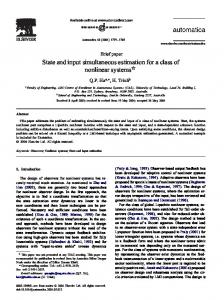
Assumption 1. wpkq and vpk jE q are uncorrelated ( x (0) −noises μ 0 )( xwith (0) −zero μ 0 )Tmeans { x(0) } = μ0 , E {white } = P0 and covariance matrices Q(4)w and Qv . Assumption 2. The state xp0q time is uncorrelated with wpkq, vpk j q and ξpk j q, andasatisfies Assuming thatinitial the sampling of the sensor is known, we consider class of non-uniform sampling discrete-time systems with missing measurements where the state updates uniformly and ! ) T the sensor samples randomly in this paper. An example of sampling time versus sensor map(4)is E txp0qu “ µ0 , E pxp0q ´ µ0 qpxp0q ´ µ0 q “ P0 depicted in Figure 1. It can be seen from Figure 1 that there are two cases when the sensor samples Assuming thatdata. the sampling timethere of theare sensor is known, we samples considerina aclass non-uniform the measurement Case 1 is that the measurement stateofupdate period sampling discrete-time systems with missing measurements where the state updates uniformly 10T ( (k − 1)T , kT ] , for example, only one measurement sample at the time instants T, 2T, 3T, 4T, 9T,and the sensor samples randomly in this paper. An example of sampling time versus sensor map and within the interval ( 4T ,5T ] with the sampling time instants k1 = 1 , k2 = 2 , k3 = 3 , k4 = 4is, depicted in Figure 1. It can be seen from Figure 1 that there are two cases when the sensor samples k11 = 9 , k12 = 10 , k5 = 4.85 , two samples in ( 7T ,8T ] with the sampling time instants k9 = 7.6 , the measurement data. Case 1 is that there are the measurement samples in a state update period k10´= 1qT, 8 , and = 5.65 samplesonly within the sampling time instants instants T,k2T, , k79T, 5T , 6T ] with sample 6 = 5.35 ppk kTs,three for example, one (measurement at the time 3T, 4T, 10T, and the interval p4T,are 5Tsno with the sampling time instants k1 period “ 1, k2 “ 3, k4, “ 4, k11 “ 9, k8 =within 6 . Case 2 is that there samples within the state update ( ( k2,−k13) T“, kT for example, k12 “ 10, k5 “ 4.85, two samples in p7T, 8Ts with the sampling time instantsk9 “ 7.6, k10 “ 8, and three not any measurement sample within ( 6T , 7T ] . samples within p5T, 6Ts with the sampling time instants k6 “ 5.35, k7 “ 5.65, k8 “ 6. Case 2 is that aim is to find the state filters at stateperiod update and measurement points based ppkpoints ´ 1q T, kTs, there Our are no samples within the state update for example, sampling not any measurement on the received measurements. sample within p6T, 7Ts.
Figure1.1.Illustration Illustrationof ofnon-uniform non-uniformsampling. sampling. Figure
3. System Modeling Our aim is to find the state filters at state update points and measurement sampling points based on theAssume received measurements. that the sensor starts to sample the measurement at the initial moment. When the sensor samples a measurement at the state update point, it is natural to take the system state at the state 3. System Modeling update point as the state at the measurement sampling point. When the sensor samples a measurement between the two state updatethe points, we adoptatthe in [9] where thethe weighted Assume that the sensor starts to sample measurement themethod initial moment. When sensor value of athe two adjacentatstates is taken as the stateitatisthe measurement sampling samples measurement the state update point, natural to take the systempoint. state at the state N k is the point. Inpoint orderas tothe facilitate let sampling number of measurement samples within a state update state atthe thealgorithm, measurement When the sensor samples a measurement k between the two state method in [9] where the weighted value of the two update interval 1) T , kT points, , and we S k =adopt ( ( k −update l =1 Nthe l is the total number of measurement samples before adjacent states is taken as the state at the measurement sampling point. the moment kT . The i ( 1 ≤ i ≤ Nk ) denotes the ith sample within the interval ( ( k − 1) T , kT . In order to facilitate the algorithm, let Nk is the number of measurement samples within a ř state update interval ppk ´ 1q T, kTs, and Sk “ kl“1 Nl is the total number of measurement samples before kT. The i (1 ď i ď Nk ) denotes the ith sample within the interval ppk ´ 1q T, kTs. Q the moment U
pk q
k “ k Sk´1 `i {T where r˚s denotes the minimal integer not less than ˚. Let αi
“ k ´ k Sk´1 `i {T, and
Sensors 2016, 16, 1155
4 of 15
pk q
pk q
then we have k Sk´1 `i “ k ´ αi . It is easily known that 0 ď αi ă 1. To simplify the expression, the sampling period T will be omitted under no confusion in the subsequent text. The state at the measurement sampling point within the interval pk ´ 1, ks is given by pk q
pk q
pk q
xpk ´ αi q “ p1 ´ αi qxpkq ` αi xpk ´ 1q
(5)
Accordingly, the measurement equation is expressed as pk q
pk q
pk q
pk q
ypk ´ αi q “ ξpk ´ αi qHxpk ´ αi q ` vpk ´ αi q
(6) pk q
Especially, when the measurement is sampled at the state update point, we have αi “ 0. Then the state at the measurement sampling point can be reduced as xpkq. The measurement equation can be reduced as ypkq “ ξpkqHxpkq ` vpkq. Assuming i and i ´ 1 are two adjacent sampling points in pk ´ 1, ks. From Equation (5), we have 1
xpkq “
pk q
α i ´1
pk q
xpk ´ αi´1 q ´ pk q
1 ´ α i ´1
pk q
xpk ´ 1q
(7)
1 ´ α i ´1
Substituting Equation (7) into Equation (5) yields pk q
pk q
pk q
xpk ´ αi q “
pk q
pαi ´ αi´1 q pk q xpk ´ α q ` xpk ´ 1q i ´ 1 pk q pk q p1 ´ αi´1 q p1 ´ αi´1 q p1 ´ αi q
(8)
Next, we construct the state space model at the measurement sampling points within a state update period. The following Theorem 1 gives the result. Theorem 1. Under Assumptions 1 and 2, the state space model at the measurement sampling points within the interval pk ´ 1, ks can be set up as follows: pk q
pk q
pk q
xpk ´ αi q “ Φi xpk ´ 1q ` Γi wpk ´ 1q pk q
pk q
(9)
pk q
pk q
ypk ´ αi q “ ξpk ´ αi qHxpk ´ αi q ` vpk ´ αi q pk q
where the coefficient matrices Φi pk q Φi
pk q
and Γi
i ´1 iÿ ´1 ź pk q “ β i ´m Φ ` m “0
pk q
with β i
pk q
l “0
pk q
(10)
are defined by ˜
l ´1 ź pk q β i ´m
¸ pk q
pk q
p1 ´ β i´l qI, Γi
“
m “0
pk q
i ´1 ź pk q β i ´m Γ
(11)
m “0
pk q
“ p1 ´ αi q{p1 ´ αi´1 q, pi ą 1q, β 1 “ 1 ´ α1 and
ś´1
m “0
pk q
β i´m “ 1.
Proof. From Equation (8), we have pk q
pk q
pk q
pk q
xpk ´ αi q “ β i xpk ´ αi´1 q ` p1 ´ β i qxpk ´ 1q
(12)
From Equation (5), we obtain pk q
pk q
pk q
xpk ´ α1 q “ β 1 xpkq ` p1 ´ β 1 qxpk ´ 1q By iterating Equation (12) and using Equation (13), we have
(13)
Sensors 2016, 16, 1155
pk q
xpk ´ αi q
pk q
where Φi
5 of 15
pk q
pk q
pk q
“ β i xpk ´ αi´1 q ` p1 ´ β i qxpk ´ 1q
pk q pk q pk q pk q pk q pk q “ β i β i´1 xpk ´ αi´2 q ` β i p1 ´ β i´1 qxpk ´ 1q ` p1 ´ β i qxpk ´ 1q pk q pk q pk q pk q pk q pk q pk q “ ¨ ¨ ¨ “ β i β i´1 ¨ ¨ ¨ β 1 xpkq ` β i β i´1 ¨ ¨ ¨ β 2 p1 ´ β 1 qxpk ´ 1q ` ¨ ¨ ¨ ` pk q pk q pk q β i p1 ´ β i´1 qxpk ´ 1q ` p1 ´ β i qxpk ´ 1q ś ř 1 ´ ś l ´1 p k q ¯ pk q pk q “ im´“10 β i´m pΦxpk ´ 1q ` Γwpk ´ 1qq ` il´ m“0 β i´m p1 ´ β i´l qxpk ´ 1q “0 pk q pk q “ Φi xpk ´ 1q ` Γi wpk ´ 1q pk q
and Γi
(14)
are defined by Equation (11). The proof is completed.
Remark 1. The model proposed in Theorem 1 establishes the relationship between the state at the measurement sampling points within the interval pk ´ 1, ks. It includes the single rate uniform sampling system as the special pk q
case, i.e., Nk “ 1 and α1 “ 0. Thus, it generalizes the standard single rate discrete-time state space model. To design the filtering algorithm, we first give a lemma to be used in the subsequent sections. Lemma 1. For system Equation (9) under ! ) Assumptions 1 and 2, the state second-order moment matrix pk q pk q T pk q q x pk ´ αi q “ E xpk ´ αi qx pk ´ αi q is computed by ´ ¯T ´ ¯T pk q q x pk ´ αi q “ Φik q x pt ´ 1q Φik ` Γik Qw Γik
(15)
The initial value is q x p0q “ µ0 µT0 ` P0 . ! ) pk q pk q pk q Proof. Substituting Equation (9) into q x pk ´ αi q “ E xpk ´ αi qxT pk ´ αi q , we easily obtain Equation (15). 4. Optimal State Estimator In this section, we will present our estimation algorithm at the state update points and measurement sampling points based on the developed model in Theorem 1. 4.1. Estimator Design Theorem 2. For system Equations (9) and (10) under Assumptions 1 and 2, the optimal estimators at the state update point and measurement sampling points in the interval pk ´ 1, ks(Nk ‰ 0) are computed by pk q
pk q
pk q
pk q
pk q
pk q
ˆ ´ αi |k ´ αi´r q “ Φi xpk ˆ ´ 1|k ´ αi´r q ` Γi wpk ˆ ´ 1|k ´ αi´r q, r “ 0, 1 xpk
(16)
where it is a filter for r “ 0 or a predictor for r “ 1. The fixed-point smoothers for the state and white noise are respectively computed by pk q
pk q
pk q
pk q
pk q
pk q
ˆ ´ 1|k ´ αi q “ xpk ˆ ´ 1|k ´ αi´1 q ` Kx pk ´ 1|k ´ αi qεpk ´ αi q xpk pk q
pk q
ˆ ´ 1|k ´ αi q “ wpk ˆ ´ 1|k ´ αi´1 q ` Kw pk ´ 1|k ´ αi qεpk ´ αi q wpk
(17) (18)
pk q
pk q
where the innovation sequence εpk ´ αi q and its covariance Qε pk ´ αi q are computed by pk q
pk q
pk q
pk q
ˆ ´ αi |k ´ αi´1 q εpk ´ αi q “ ypk ´ αi q ´ γH xpk
(19)
Sensors 2016, 16, 1155
6 of 15
pk q
pk q
pk q
pk q
Qε pk ´ αi q “ γ2 HPx pk ´ αi |k ´ αi´1 qH T ` γp1 ´ γqHq x pk ´ αi qH T ` Qv pk q
(20)
pk q
The smoothing gain matrices Kx pk ´ 1|k ´ αi q for the state and Kw pk ´ 1|k ´ αi q for the white noise are computed by pk q
pk q
p k qT
Kx pk ´ 1|k ´ αi q “ γrPx pk ´ 1|k ´ αi´1 qΦi pk q
pk q
pk q
p k qT
pk q
pkqT
` Pxw pk ´ 1|k ´ αi´1 qΓi
pkqT
Kw pk ´ 1|k ´ αi q “ γrPwx pk ´ 1|k ´ αi´1 qΦi
pk q
(21)
pk q
(22)
1 sH T Q´ ε pk ´ αi q
` Pw pk ´ 1|k ´ αi´1 qΓi
1 sH T Q´ ε pk ´ αi q
pk q
pk q
The smoothing error covariance matrices Px pk ´ 1|k ´ αi q and Pw pk ´ 1|k ´ αi q, and the pk q
cross-covariance matrix Pxw pk ´ 1|k ´ αi q for the state and white noise are computed by pk q
pk q
pk q
pk q
pk q
pk q
pk q
pk q
pk q
Px pk ´ 1|k ´ αi q “ Px pk ´ 1|k ´ αi´1 q ´ Kx pk ´ 1|k ´ αi qQε pk ´ αi qKTx pk ´ 1|k ´ αi q
(23)
pk q
T Pw pk ´ 1|k ´ αi q “ Pw pk ´ 1|k ´ αi´1 q ´ Kw pk ´ 1|k ´ αi qQε pk ´ αi qKw pk ´ 1|k ´ αi q
pk q
pk q
pk q
pk q
(24)
pk q
T Pxw pk ´ 1|k ´ αi q “ Pxw pk ´ 1|k ´ αi´1 q ´ K x pk ´ 1|k ´ αi qQε pk ´ αi qKw pk ´ 1|k ´ αi q
pk q
(25)
pk q
The filtering (r “ 0) and prediction (r “ 1) error covariance matrices Px pk ´ αi |k ´ αi´r q for the state are computed by pk q
pk q
pk q
pk q
pkqT
Px pk ´ αi |k ´ αi´r q “ Φi Px pk ´ 1|k ´ αi´r qΦi pk q pk q pkqT Φi Pxw pk ´ 1|k ´ αi´r qΓi
pk q
pk q pk q p k qT ` Γi Pwx pk ´ 1|k ´ αi´r qΦi ,
pk q
pk q
pk q
pkqT
` Γi Pw pk ´ 1|k ´ αi´r qΓi
`
(26)
r “ 0, 1 pk q
The initial values are Px pk ´ 1|k ´ α0 q “ Px pk ´ 1|k ´ 1q, Pw pk ´ 1|k ´ α0 q “ Qw , Pxw pk ´ 1|k ´ pk q
pk q
ˆ ´ 1|k ´ α0 q “ xpk ˆ ´ 1|k ´ 1q and wpk ˆ ´ 1|k ´ α0 q “ 0. α0 q “ 0, xpk
pk q
pk q
ˆ ˆ ´ α N |k ´ α N q when It is clear that we have the estimator at the state update point as xpk|kq “ xpk k
pk q
pk q
ˆ ˆ ´ αN α N “ 0 or xpk|kq “ xpk k
k`1
pk q
pk q
|k ´ α N q with α N k
k`1
pk q
“ 0, and β N
k`1
k
pk q
pk q
k
k
“ 1{p1 ´ α N q when α N ‰ 0.
Proof. See Appendix A. pk q
Remark 2. In Theorem 2, if Nk “ 1 and α1 “ 0, we have the filtering algorithm at the state update points for single-rate systems. If Nk “ 0, i.e., no samples in the interval pk ´ 1, ks, the predictor is used to estimate the state at the state update point k based on the estimator at the state update point k ´ 1. Remark 3. It can be easily known that the proposed non-augmented recursive estimator has the computational order of magnitude OpNk p3 q in the interval pk ´ 1, ks. Compared with the augmented estimator [9] with the computational order of magnitude OpNk3 q3 q, our algorithm can obviously reduce the computational cost with the increase of the number Nk of measurement samples in the interval pk ´ 1, ks for a deterministic system with the fixed p and q. Meanwhile, it is more important that our filter can give the estimates not only at the state update points but also at the measurement sampling points within a state update period in real time. However, the estimator of [9] can only give the estimates at the state update points. 4.2. Computational Procedures of the Estimator Based on Theorem 1 and Theorem 2, the computational procedures of our estimator at the state update points and at the measurement sampling points are addressed as follows: ˆ Step 1. k “ 1, set the initial values xp0|0q “ µ0 , Px p0|0q “ P0 , Pw p0|0q “ Qw , Pxw p0|0q “ 0 and q x p0q “ µ0 µT0 ` P0 . Step 2. Construct the model within a state update period pk ´ 1, ks by Theorem 1.
Sensors 2016, 16, 1155
7 of 15
Step 3. Compute the state estimators at the state update points and at the measurement sampling points: (a)
If Nk ‰ 0 (i.e., there are samples within a state update period), obtain the state estimates pk q
pk q
pk q
pk q
ˆ ´ αi |k ´ αi q and the covariance matrices Px pk ´ αi |k ´ αi q by Theorem 2. xpk (b) If Nk “ 0 (i.e., no sample within a state update period), obtain the estimate by prediction method ˆ ˆ ´ 1|k ´ 1q, Px pk|kq “ ΦPx pk ´ 1|k ´ 1qΦT ` ΓQw ΓT . in Remark 2, i.e., xpk|kq “ Φ xpk pk q
pk q
pk q
Step 4. k “ k ` 1, set Px pk ´ 1|k ´ α0 q “ Px pk ´ 1|k ´ 1q, Pw pk ´ 1|k ´ α0 q “ Qw , Pxw pk ´ 1|k ´ pk q
pk q
ˆ ´ 1|k ´ α0 q “ xpk ˆ ´ 1|k ´ 1q and wpk ˆ ´ 1|k ´ α0 q “ 0. α0 q “ 0, xpk Go to Step 2. 5. Multi-Sensor Case In the preceding section, we have presented a non-augmented optimal recursive estimator for single sensor system. In this section, we will discuss how to use the proposed algorithm to solve the multi-sensor case. For a multi-sensor system, the state equation is the same as Equation (1) and the measurement equations are given as follows: pl q
pl q
pl q
pl q
ypl q pk j q “ ξ pl q pk j qH pl q xpk j q ` vpl q pk j q
(27) pl q
where the superscript l denotes the lth sensor, L is the number of sensors, ypl q pk j q is the measurement pl q
pl q
pl q
at the sampling time k j for the lth sensor, k j is the sampling time of the jth measurement, vpl q pk j q is the measurement noise with zero mean and covarianceQvplq , and H pl q is the measurement matrix. The pl q
variable ξ pl q pk j q is a Bernoulli distributed stochastic variable that takes values on 1 and 0 with the ! ) pl q pl q probability Prob ξ pl q pk j q “ 1 “ γpl q , γpl q P r0, 1s. We assume that ξ pl q pk j q is independent of wpkq pl q
pl q
and vpl q pk j q and xp0q. Moreover ξ pl q pk j q satisfies that pl q
pl q
2
Etξ pl q pk j u “ γpl q , Etpξ pl q pk j ´ γpl q q u “ γpl q p1 ´ γpl q q, Etξ pl q pklj q ´ γpl q u “ 0, pl q
pl q
pl q
psq
pl q
Etξ pl q pk j qp1 ´ ξ pl q pk j qqu “ 0, Etξ pl q pk i qξ psq pm j qu “ γpl q γpsq pl ‰ s or k i
psq
(28)
‰ mj q
We will adopt two types of methods to deal with the estimation problem of multi-sensor case: optimal fusion estimator and suboptimal fusion estimator. 5.1. Optimal Fusion Estimator pl q In fact, we can reorder the measurements ypl q pk j q of all sensors in each state update period pl q
pk ´ 1, ks according to the order of sampling time k j . If the sampling time of measurements from some sensors is same, i.e., sampling at the same time point, they will be combined to an augmented measurement at this sampling time. These reorder measurements can be considered from a certain single sensor. Then, our estimation algorithm in Section 4 can be applied to the optimal fusion estimation problem of multiple sensors. When all sensors work healthily, the proposed optimal fusion algorithm can obtain the best accuracy. However, it has bad reliability, which means that a faulty sensor can lead to the optimal fusion estimator to diverge [26]. To improve the reliability, we give the following distributed suboptimal fusion algorithm.
Sensors 2016, 16, 1155
8 of 15
5.2. Suboptimal Fusion Estimator Firstly, apply our estimation algorithm in this paper to obtain the local estimators at the state update points based on the measurements from individual sensors, and then apply the covariance intersection (CI) fusion algorithm [27,28] to obtain the distributed suboptimal fusion estimator at the state update points. The reason that we adopt CI algorithm is that it avoids the computation of cross-covariance matrices between any two local estimators [26]. The CI fusion estimator can be given as follows [27,28]: L ” ı´1 ÿ pl q xˆCI pk|kq “ ω pl q pkqPCI pk|kq Px pk|kq xˆ pl q pk|kq (29) l “1
« PCI pk|kq “
L ÿ
ω
pl q
´1 pl q pkqrPx pk|kqs
ff´1 (30)
l “1
where PCI pk|kq is the upper bound of variance of the CI fusion estimator. The optimal weighted ř coefficients ω pl q pkq satisfy 0 ď ω pl q pkq ď 1 and lL“1 ω pl q pkq “ 1, and can be obtained by solving the following optimization problem: řL l“1
min ω plq pkq“1,0ďω plq pkqď1
trpPCI pk|kqq
(31)
The nonlinear optimization problem Equation (29) does not generally have the analytical solutions. It can be solved by numerical methods, which can be carried out by the function “fmincon” in Matlab optimization toolbox. It only involves the scalar optimization problem. The proposed distributed CI fusion estimator has the advantage of good robustness and flexibility, i.e., good reliability since it has the distributed parallel structure that is convenient for detection and isolation of a faulty sensor. Certainly, when all sensors work healthily, it has worse accuracy than the optimal fusion estimator. However, it has better accuracy than local estimators [27,28]. Remark 4. The proposed optimal fusion algorithm is a non-augmented method. Certainly, we can also use the centralized fusion way [9] that combines the measurements from all sensors within a state update period into an augmented measurement and then use standard Kalman filter to solve. However, it is well known that this way has the expensive computational burden with the increase of the number of sensors [26]. 6. Simulation Research In this section, a spring-mass system that has been widely adopted in many studies [29–31] will be used to verify the effectiveness of our algorithms: »
0 0
0 0
k2 M2
k2 M1 k2 ´M 2
— . — xptq “ — k1 `k2 – ´ M1
1 0 ´M
0 1 0
0
´ M2
µ 1
µ
fi
»
fi 0 ffi — 0 ffi ffi — ffi ffi xptq ` — 1 ffi wptq fl – M1 fl
(32)
1 M2
” ıT . . where xptq “ x1 ptq x2 ptq x1 ptq x2 ptq , x1 and x2 are the positions of mass M1 and mass M2 , respectively; k1 and k1 are the spring constants of spring 1 and spring 2, respectively; and µ denotes the viscous friction coefficient between the mass blocks and the horizontal surface. Moreover, the pi q measurement equations are given as Equation (27) with L = 3. vpiq pk j q, i “ 1, 2, 3 are independent Gaussian noises with zero means and variances Qvpiq and uncorrelated with the process”noise wpkq with ı zero-mean and variance Qw . We set Qw “ 2, Qvp1q “ 2, Qvp2q “ 1, Qvp3q “ 3, H p1q “ 1 1 1 0 , ” ı ” ı H p2q “ 0 1 0 0 , H p3q “ 0 0 1 1 , γp1q “ 0.7, γp2q “ 0.9, γp3q “ 0.8, M1 “ 1, M2 “ 0.5,
Sensors 2016, 16, 1155
9 of 15
k1 “ 1, k2 “ 1, µ “ 0.5, and the sampling period T “ 0.1 s, we obtain the following system parameter matrices by discretization: » fi » fi 0.9902 0.0049 0.0972 0.0002 0.0049 — 0.0096 — 0.0097 ffi 0.9903 0.0003 0.0948 ffi — ffi — ffi Φ“— (33) ffi , Γ “ — ffi – ´0.1941 0.0969 0.9416 0.0047 fl – 0.0975 fl 0.1891 ´0.1894 0.0095 0.8955 0.1900 We set the initials as xp0q “ 0 and P0 “ 0.1I4 . We take 100 sampling data. Figure 2 gives the sketch map of the sampling data of the three sensors within the time interval 0–20. Figure 3 gives the tracking performance of the optimal fusion estimator, where the solid curves denote the true values and the dashed ones denote the estimators. Figure 4 gives the comparisons curves of the traces of variances for local estimators and the fusion estimators. From Figure 4, we can see that our optimal fusion estimator has best accuracy and CI fusion estimator has better accuracy Sensors 2016, 16, 1155 9 of 14 than local estimators.
(a)
(b)
(c) Figure 2. Samples of sensors 1–3 ofthe thefirst firstsensor; sensor; samples of second the second Figure 2. Samples of sensors 1–3inin[1,20]: [1,20]: (a) (a) samples samples of (b)(b) samples of the sensor; (c) samples the thirdsensor. sensor. sensor; andand (c) samples of of the third
Then Monte Carlo simulation is carried out to compare the algorithms in our paper and [9]. N 2 ř j j The mean square errors (MSEs): MSEi,s pkq “ N1 pxi pkq ´ xˆi,s pk|kqq , i=1, 2, 3, 4; s=our paper, [9]) will j “1
be used to evaluate the estimation performance of the two estimation algorithms, where the subscript i denotes the ith components and s denotes our filter or that in [9], respectively, and N is the number of Monte Carlo runs.
(c) Figure 2. Samples of sensors 1–3 in [1,20]: (a) samples of the first sensor; (b) samples of the second 10 of 15 sensor; and (c) samples of the third sensor.
Sensors 2016, 16, 1155
(a)
(b)
(c)
(d)
; (b) tracking position Figure 3. Optimal fusion estimator: theposition positionofof Figure 3. Optimal fusion estimator:(a) (a)tracking tracking for for the MM tracking for for the the position of of 1 ; 1(b) Sensors 2016, 16,2tracking 10 of 14 M ; 1155 (c) tracking velocity ; and(d) (d)tracking tracking for MM . for for thethe velocity ofofMM 1;1and forthe thevelocity velocityofof 2 . M2; (c) 2
Figure 4. Comparison of the traces local estimators fusion estimators. Figure 4. Comparison of the tracesof ofvariances variances ofoflocal estimators andand fusion estimators.
Then In Monte simulation is carried out totocompare thealgorithms algorithms in paper our paper and FigureCarlo 5, the sensor 1 is randomly employed compare the in our and [9]. The[9]. The N Carlo runs is shown in Figure 5. Because Yan, L. et al. [9] comparison of MSEs simulated by 100 Monte 1 j mean square (MSEs): 3, 4; paper, [9]) will be k )) 2 , i=1, MSE ( xij ( k ) − xˆfrom i , s ( k ) = measurements, i , s ( k |Figure does noterrors consider the effect of missing 5, we2,can sees=our that the proposed N j =1 algorithm has better accuracy than the one in [9] when the missing measurements occur in sensors.
used to evaluate the estimation performance of the two estimation algorithms, where the subscript i denotes the ith components and s denotes our filter or that in [9], respectively, and N is the number of Monte Carlo runs. In Figure 5, the sensor 1 is randomly employed to compare the algorithms in our paper and [9]. The comparison of MSEs simulated by 100 Monte Carlo runs is shown in Figure 5. Because Yan, L et al [9] does not consider the effect of missing measurements, from Figure 5, we can see that the proposed algorithm has better accuracy than the one in [9] when the missing measurements occur in
In Figure 5, the sensor 1 is randomly employed to compare the algorithms in our paper and [9]. The comparison of MSEs simulated by 100 Monte Carlo runs is shown in Figure 5. Because Yan, L et al [9] does not consider the effect of missing measurements, from Figure 5, we can see that the proposed algorithm has better accuracy than the one in [9] when the missing measurements occur in Sensors 2016, 16, 1155 11 of 15 sensors.
(a)
(b)
(c)
(d)
Figure 5. 5. Comparison the estimators estimatorsininthis this paper [9] sensor for sensor (a) MSEs Figure ComparisonofofMSEs MSEs of of the paper andand [9] for 1: (a)1:MSEs of the of the 1 ; (b) MSEs of the position estimators of M 2 ; (c) MSEs of the velocity estimators position estimators of M position estimators of M1 ; (b) MSEs of the position estimators of M2 ; (c) MSEs of the velocity estimators ; and (d)(d) MSEs of M of1M MSEsofofthe thevelocity velocity estimators estimators ofofMM 1 ; and 2 .2.
Next, we will make the comparison with [9] when there are no missing measurements. The sensor 1 is employed with γp1q “ 1 in simulation. Figure 6 gives the comparison of MSEs simulated by 100 Monte Carlo runs for the estimators in this paper and [9]. In Figure 6, the estimates at the state update points and the measurement sampling points within a state update period are all shown by using the our proposed algorithm. Moreover, from Figure 6, we can see that the proposed algorithm has the same accuracy as the augmented one in [9] at the state update points when there are no missing measurements. It is also significant from Remark 3 that our estimator has smaller computational burden than [9]. To compare the computation time between the two algorithms, we use the “unifrnd” function in Matlab to sample 2, 3, 4, and 5 measurements within a state update period, respectively, and give the average of 50 run time of the two algorithms in Table 1. The used computer is Lenovo with the CPU speed of 3.20 GHz (Intel (R) Core (TM) i5-3470 CPU) and the used Matlab version is Matlab R2012a. From Table 1, we can see that our proposed algorithm can save the run time compared with that in [9] with the increase of the number of sampling points within a state update period.
in Matlab to sample 2, 3, 4, and 5 measurements within a state update period, respectively, and give the average of 50 run time of the two algorithms in Table 1. The used computer is Lenovo with the CPU speed of 3.20 GHz (Intel (R) Core (TM) i5-3470 CPU) and the used Matlab version is Matlab R2012a. From Table 1, we can see that our proposed algorithm can save the run time compared with that in [9] Sensors 2016, 16, 1155 12 of 15 with the increase of the number of sampling points within a state update period.
(a)
(b)
(c)
(d)
Figure 6. 6.Comparison of the theestimators estimatorsinin this paper [9]sensor for sensor 1 without missing Figure Comparisonof of MSEs MSEs of this paper andand [9] for 1 without missing 1 ; (b) MSEs of the position estimators measurements: (a) MSEs of the position estimators of M measurements: (a) MSEs of position estimators of M1 ; (b) MSEs of the position estimators of M2 ; of M2; MSEs thevelocity velocity estimators estimators ofofMM MSEs of the velocity estimators of M2of . M 2. and(d)(d) MSEs of the velocity estimators (c)(c) MSEs ofofthe 1 ;1;and Table time of 50 Table1.1.Average Average time of runs. 50 runs.
Number Numberof ofSamples Samples 22 33 4 45 5
Our OurAlgorithm Algorithm 0.062064 0.062064 s s 0.078872 s 0.078872 s 0.092339 s 0.092339 0.103354 s s 0.103354 s
[9] [9]
0.066064 0.066064 s 0.086958 s 0.086958 0.112633 s 0.112633 0.146654 s
s s s 0.146654 s
7. Conclusions
7. Conclusions A non-augmented recursive estimator has been designed for a class of non-uniform sampling systems with missing recursive measurements, where system state for is updated and sampling the A non-augmented estimator hasthe been designed a class ofuniformly non-uniform measurements are sampled randomly. A state space is constructed to depict the dynamics and at systems with missing measurements, where themodel system state is updated uniformly the the measurement sampling points within a state update period. The proposed estimator dependent on the missing rate can provide the state estimates not only at the state update points but also at the measurement sampling points within a state update period. Compared with [9], our algorithm has better accuracy when there are missing measurements and the same accuracy at the state update points when there are no missing measurements. For multi-sensor systems with missing measurements, our algorithm can also deal with the optimal fusion estimation by reordering the measurements from all sensors. A distributed suboptimal fusion estimator is also given using the covariance intersection (CI) fusion algorithm.
Sensors 2016, 16, 1155
13 of 15
Acknowledgments: This work was supported by the National Natural Science Foundation of China under Grant No. 61174139, 61573132, the Heilongjiang Province Outstanding Youth fund (No. JC201412), Chang Jiang Scholar Candidates Program for Provincial Universities in Heilongjiang (No. 2013CJHB005), and the Program for Graduate Innovation Scientific Research of Heilongjiang University (YJSCX2015-001HLJU). Author Contributions: Shuli Sun proposed the algorithm and wrote the paper. Honglei Lin derived the algorithm and performed the simulation work. Conflicts of Interest: The authors declare no conflict of interest.
Appendix A. The Proof of Theorem 2 By using the projection theory [32], we readily have Equations (16)–(19), where the filtering gain matrices for the state and input white noise are, respectively, defined as ! ) pk q pk q pk q 1 Kx pk ´ 1|k ´ αi q “ E xpk ´ 1qεT pk ´ αi q Q´ ε pk ´ αi q
(A1)
! ) pk q pk q pk q 1 Kw pk ´ 1|k ´ αi q “ E wpk ´ 1qεT pk ´ αi q Q´ ε pk ´ αi q
(A2)
pk q
Substituting Equation (10) into Equation (19), the innovation εpk ´ αi q can be rewritten as pk q pk q pk q pk q pk q pk q εpk ´ αi q “ pξpk ´ αi q ´ γqHxpk ´ αi q ` γH xrpk ´ αi |k ´ αi´1 q ` vpk ´ αi q
(A3)
pk q pk q pk q pk q pk q ˆ ´ αi |k ´ αi´1 q. Substituting where the prediction error xrpk ´ αi |k ´ αi´1 q “ xpk ´ αi q ´ xpk ! ) pk q pk q pk q Equation (A3) into the innovation sequence covariance Qε pk ´ αi q “ E εpk ´ αi qεT pk ´ αi q leads to Equation (20). Subtracting Equation (16) with r “ 1 from Equation (9) yields the prediction error equation pk q pk q pk q pk q pk q kq r ´ 1|k ´ αpi´ xrpk ´ αi |k ´ αi´1 q “ Φi xrpk ´ 1|k ´ αi´1 q ` Γi wpk 1q
(A4)
pk q pk q kq r ´ 1|k ´ αpi´ ˆ ´ 1|k ´ αi´1 q and wpk where the smoothing errors xrpk ´ 1|k ´ αi´1 q “ xpk ´ 1q ´ xpk 1q “ pk q
ˆ ´ 1|k ´ αi´1 q. Using Equations (A3) and (A4), we have wpk ´ 1q´ wpk ! ) ´ ¯T * pkq pkq pkq pkq r ´ 1|k ´ αpkq E xpk ´ 1qεT pk ´ αi q “ γE txpk ´ 1q Φi xrpk ´ 1|k ´ αi´1 q `Γi wpk q HT i´1 pkq
pkqT
“ γrPx pk ´ 1|k ´ αi´1 qΦi
pkq
pkqT
` Pxw pk ´ 1|k ´ αi´1 qΓi
(A5)
sH T
pk q pk q pk q pk q ˆ ´ 1|k ´ αi´1 q ` xrpk ´ 1|k ´ αi´1 q, xpk ˆ ´ 1|k ´ αi´1 qKxrpk ´ 1|k ´ αi´1 q and where xpk ´ 1q “ xpk pkq kq r pk ´ 1|k ´ αpi´ xˆ pk ´ 1|k ´ αi´1 qK w 1 q have been used, where the symbol K denotes orthogonality. Substituting Equation (A5) into Equation (A1) yields Equation (21). Similarly, we prove Equation (22) holds. Subtracting Equation (17) from xpk ´ 1q yields the smoothing error equation pkq pkq pkq pkq r xpk ´ 1|k ´ αi q “ r xpk ´ 1|k ´ αi´1 q ´ Kx pk ´ 1|k ´ αi qεpk ´ αi q
(A6)
The smoothing error covariance matrix is derived as follows: ! ) pkq pkq T pkq Px pk ´ 1|k ´ αi q “ E r xpk ´ 1|k ´ αi qr x pk ´ 1|k ´ αi q pkq
pkq
pkq
pkq
“ Px pk ´ 1|k!´ αi´1 q ` Kx pk ´ 1|k ´ αi qQ)ε pk ´ αi qKxT pk ´ 1|k ´ αi q pkq pkq pkq ´E r xpk ´ 1|k ´ αi´1 qεT pk ´ αi q KxT pk ´ 1|k ´ αi q ! ) pkq pkq T pkq ´Kx pk ´ 1|k ´ αi qE εpk ´ αi qr x pk ´ 1|k ´ αi´1 q Using Equation (A1) and note that
(A7)
Sensors 2016, 16, 1155
14 of 15
! ) ! ) pkq pkq pkq pkq pkq E r xpk ´ 1|k ´ αi´1 qεT pk ´ αi q “ E xpk ´ 1qεT pk ´ αi q “ Kx pk ´ 1|k ´ αi qQε pk ´ αi q
(A8)
Substituting Equation (A8) into Equation (A7) leads to Equation (23). Similarly, we can prove Equations (24) and (25) hold. Subtracting Equation (16) with r “ 0 from Equation (9) yields the filtering error equation pkq pkq pkq pkq pkq r r pk ´ 1|k ´ αpi kq q xpk ´ αi |k ´ αi q “ Φi r xpk ´ 1|k ´ αi q ` Γi w
(A9)
pkq pkq pkq pkq Substituting Equations (A4) and (A9) into Px pk ´ αi |k ´ αi´r q “ Etr xpk ´ αi |k ´ αi´r q pkq pkq r xT pk ´ αi |k ´ αi´r qu, r “ 0, 1 leads to Equation (26). This proof is completed.
References 1. 2. 3. 4. 5. 6. 7. 8.
9. 10. 11.
12. 13.
14. 15. 16.
Ding, F.; Liu, G.; Liu, X. Partially coupled stochastic gradient identification methods for non-uniformly sampled systems. IEEE Trans. Autom. Control 2010, 55, 1976–1981. [CrossRef] Li, W.; Shah, S.; Xiao, D. Kalman filters in non-uniformly sampled multirate systems: For FDI and beyond. Automatica 2008, 44, 199–208. [CrossRef] Yan, L.; Liu, B.; Zhou, D. Asynchronous multirate multisensor information fusion algorithm. IEEE Trans. Aerosp. Electron. Syst. 2007, 43, 1135–1146. [CrossRef] Yan, L.; Zhou, D.; Fu, M.; Xia, Y. State estimation for asynchronous multirate multisensor dynamic systems with missing measurements. IET Signal Process. 2010, 4, 728–739. [CrossRef] Yan, L.; Li, X.; Xia, Y.; Fu, Y. Modeling and estimation of asynchronous multirate multisensor system with unreliable measurements. IEEE Trans. Aerosp. Electron. Syst. 2015, 51, 2012–2026. [CrossRef] Lin, H.; Ma, J.; Sun, S. Optimal state filters for a class of non-uniform sampling systems. J. Syst. Sci. Math. Sci. 2012, 32, 768–779. Mahmoud, M.S.; Emzir, M.F. State estimation with asynchronous multirate multismart sensors. Inform. Sci. 2012, 196, 15–27. [CrossRef] Ma, J.; Lin, H.; Sun, S. Distributed fusion filter for asynchronous multi-rate multi-sensor non-uniform sampling systems. In Proceedings of the 15th International Conference on Information Fusion, Singapore, Singapore, 9–12 July 2012; pp. 1645–1652. Yan, L.; Xiao, B.; Xia, Y.; Fu, M. State estimation for a kind of non-uniform sampling dynamic system. Int. J. Syst. Sci. 2013, 44, 1913–1924. [CrossRef] Hu, Y.; Duan, Z.; Zhou, D. Estimation fusion with general asynchronous multirate sensors. IEEE Trans. Aerosp. Electron. Syst. 2010, 46, 2090–2101. [CrossRef] Xu, S.; Lin, X.; Fu, M.; Zhao, D. Multi-rate sensor adaptive data fusion algorithm based on incomplete measurement. In Proceedings of the IEEE International Conference on Automation and Logistics, Chongqing, China, 15–16 August 2011; pp. 448–491. Peng, F.; Sun, S. Distributed fusion estimation for multisensor multirate systems with stochastic observation multiplicative noises. Math. Probl. Eng. 2014, 2014. [CrossRef] Ma, J.; Sun, S. Distributed Fusion Filter for Multi-rate Multi-sensor Systems with Packet Dropouts. In Proceedings of the 10th World Congress on Intelligent Control and Automation, Beijing, China, 6–8 July 2012; pp. 4502–4506. Zhang, W.; Feng, G.; Yu, L. Multi-rate distributed fusion estimation for sensor networks with packet losses. Automatica 2012, 48, 2016–2028. [CrossRef] Liang, Y.; Chen, T.; Pan, Q. Multi-rate stochastic H8 filtering for networked multisensor fusion. Automatica 2010, 46, 437–444. [CrossRef] Geng, H.; Liang, Y.; Zhang, X. Linear-minimum-mean-square-error observer for multi-rate sensor fusion with missing measurements. IET Control Theory Appl. 2014, 8, 1375–1383. [CrossRef]
Sensors 2016, 16, 1155
17.
18. 19. 20. 21. 22. 23. 24.
25. 26. 27. 28. 29. 30. 31. 32.
15 of 15
Zhang, W.; Liu, S.; Chen, M.; Yu, L. Fusion estimation for two sensors with nonuniform estimation rates. In Proceedings of the 51st IEEE Conference on Decision Control, Maui, HI, USA, 10–13 December 2012; pp. 4083–4088. Zhang, W.; Liu, S.; Yu, L. Fusion estimation for sensor networks with nonuniform estimation rates. IEEE Trans. Circuits Syst. I Reg. Pap. 2014, 61, 1485–1498. [CrossRef] Talebi, H.; Hemmatyar, A.M.A. Asynchronous track-to-track fusion by direct estimation of time of sample in sensor networks. IEEE Sens. J. 2014, 14, 210–217. [CrossRef] Song, H.; Zhang, W.; Yu, L. Hierarchical fusion in clustered sensor networks with asynchronous local estimates. IEEE Signal Process. Lett. 2014, 21, 1506–1510. [CrossRef] Chen, B.; Zhang, W.; Yu, L. Distributed fusion estimation with missing measurements, random transmission delays and packet Dropouts. IEEE Trans. Autom. Control 2014, 59, 1961–1967. [CrossRef] Ma, J.; Sun, S. Centralized fusion estimators for multisensor systems with random sensor delays, multiple packet dropouts and uncertain observations. IEEE Sens. J. 2013, 13, 1228–1235. [CrossRef] Ma, J.; Sun, S. Optimal linear estimators for systems with random sensor delays, multiple packet dropouts and uncertain observations. IEEE Trans. Signal Process. 2011, 59, 5158–5192. Moayedi, M.; Foo, Y.K.; Soh, Y.C. Adaptive Kalman filtering in networked systems with random sensor delays, multiple packet dropouts and missing measurements. IEEE Trans. Signal Process. 2010, 58, 1577–1588. [CrossRef] Lin, H.; Sun, S. State estimation for a class of non-uniform sampling systems. In Proceedings of the 34th Control Conference, Hangzhou, China, 28–30 July 2015; pp. 2024–2027. Sun, S.; Deng, Z. Multi-sensor optimal information fusion Kalman filter. Automatica 2004, 40, 1017–1023. [CrossRef] Julier, S.J.; Uhlmann, J.K. General decentralized data fusion with covariance intersection. In Handbook of Multisensor Data Fusion; CRC Press: Boca Raton, FL, USA, 2001; pp. 319–342. Deng, Z. Information Fusion Estimation Theory with Application; Science Press: Beijing, China, 2012. Song, H.; Yu, L.; Zhang, W. Networked H8 filtering for linear discrete-time systems. Inf. Sci. 2011, 181, 686–696. [CrossRef] Gao, H.; Chen, T. H8 estimation for uncertain systems with limited communication capacity. IEEE Trans. Autom. Control 2007, 52, 2070–2084. [CrossRef] Ma, J.; Sun, S. Optimal linear estimators for multi-sensor stochastic uncertain systems with packet losses of both sides. Digit. Signal Process. 2015, 37, 24–34. [CrossRef] Anderson, B.D.O.; Moore, J.B. Optimal Filtering; Prentice-Hall: Englewood Cliffs, NJ, USA, 1979. © 2016 by the authors; licensee MDPI, Basel, Switzerland. This article is an open access article distributed under the terms and conditions of the Creative Commons Attribution (CC-BY) license (http://creativecommons.org/licenses/by/4.0/).