Since particle filters can be used in non-Gaussian and nonlinear system models, they have a wider range of ap- plications than Kalman filters. In this paper, a ...
Electronics and Communications in Japan, Vol. 98, No. 6, 2015 Translated from Denki Gakkai Ronbunshi, Vol. 133-C, No. 7, July 2013, pp. 1376–1379
State Feedback Control Using Particle Filter
TAKESHI NISHIDA Kyushu Institute of Technology, Kitakyushu City, Fukuoka Prefecture, Japan
an outdoor mobile robot, a variety of results have been reported [3, 4]. However, in most existing research using PF, high-level control systems1 such as tracking systems or user interfaces have been the focus, and there have been few reports on their use in low-level systems2 such as motor control systems. In general, minimum mean square estimation (MMSE) or maximum a-posteriori (MAP) estimation is used to extract a unique estimated value (also referred to as a characteristic value) from a-posteriori estimations made with a PF. Because these quantities can be actively calculated as weighted averages for the particles, they are used as characteristic values in various kinds of research. However, when the estimates are made for a nonGaussian distribution, they do not constitute appropriate characteristic values [5]. In practical applications, there are many cases in which the a-posteriori distribution is multimodal. In such cases, the MMSE is calculated in regions with very small values of the a-posteriori probability density, i.e., at peaks and the troughs between peaks. Although amount of computation increases in these cases, highly reliable characteristic values are provided for non-Gaussian distributions [5–7]. In earlier research on the use of PF for state estimation in low-level systems [8–10], MMSE is used as a method of extracting a unique deterministic state required for feedback. Thus, it is not a method that reflects the maximal features of the PF by which a multimodal probability distribution can be approximated, and thus is not superior to a KF. Thus, this paper proposes a method of using a PF as an observer for a low-level control system that includes multimodal probabilistic noise. In this method, more reliable estimates are obtained by introducing pf-MAP [5] as a MAP estimation method for the multimodal probability distributions estimated with a PF. The ESS method is also introduced [11] in order to adjust the resampling frequency
SUMMARY Since particle filters can be used in non-Gaussian and nonlinear system models, they have a wider range of applications than Kalman filters. In this paper, a construction method for a state feedback control system using a particle filter as an observer for probabilistic state estimation is described. In order to assure robustness to non-Gaussian noise, a maximum a-posteriori probability estimation extraction method and an method for evaluation of the effective sample size have been incorporated into the particle filter. The effectiveness of the constructed system was verified experimentally, and the effectiveness of the state observer constructed with the particle filter is demonstrated through a comparison with a Kalman filter. C⃝ 2015 Wiley Periodicals, Inc. Electron Comm Jpn, 98(6): 16–25, 2015; Published online in Wiley Online Library (wileyonlinelibrary.com). DOI 10.1002/ecj.11658 Key words: Kalman filter; observer; particle filter; state estimation; state feedback control system.
1.
Introduction
Kalman filters (KF), extended Kalman filters (EKF), and unscented Kalman filters (UKF) have long since been used as state estimation methods that explicitly use probabilistic noise in a state feedback control system. However, these KFs assume Gaussian characteristics of the probabilistic noise, and consequently appropriate state estimation cannot be performed when non-Gaussian probabilistic noise is included. In contrast, particle filters (PF) can be used in nonlinear and non-Gaussian models, and state estimation of a greater variety of systems can be performed than with KF. Thus, in recent years they have been used in many fields [1, 2]. As a typical example, in applied research on the simultaneous localization and mapping (SLAM) problem, in which estimation of state properties and automatic mapping are performed simultaneously by
1 Control systems with a high degree of abstraction relative to physical quantities in the real world. 2 Control system in with a lower degree of abstraction relative to physical quantities in the real world is lower than in high-level control system.
C⃝
16
2015 Wiley Periodicals, Inc.
and to create an appropriate particle distribution with the variation of the observation noise taken into consideration. In addition, in a system including multimodal probabilistic noise, which is difficult for a KF to estimate accurately, we show through simulations that system stabilization can be achieved by means of the state feedback utilized in the present method. Simulations verifying the effects of the pfMAP and ESS methods and the relationship between the PF particle count, the computational burden, and estimation precision are also presented. This paper is organized as follows. First, in Section 2 the procedure of the PF algorithm proposed in this paper is given, and in Section 3 a method of creating a control system with a PF used in the state feedback control system is presented. Next, in Section 4 the effectiveness of the proposed method is evaluated by comparison with a KF based on numerical simulations. Finally, Section 5 concludes the paper.
2.
the frequency of resampling. For instance, if resampling is frequent in the presence of multimodal probabilistic noise, the particles may collect only in regions with strong peaks. By appropriately reducing the frequency of resampling in the ESS method, the particles can be arranged more widely. Algorithm 1. Particle Filter 1: loop 2: 3:
π ˜k
5:
end for
6:
π ˜k
y k = h k (x k , 𝛇k )
(2)
(m)
:= π ˜k
M i=1
/
8:
ESS = 1/
9:
for m := 1 to M do
M i=1
)
//Sampling step //Likelihood evaluation step
(i)
π ˜k
(i) 2
πk
//calculation of ESS
if ESS < ⎧ ESSth then (1) ⎪ ˜ (1) with prob. π ˜k ⎪ k ⎪x ⎪ ⎨ . . (m) . xk ∼ . . ⎪. ⎪ ⎪ ⎪ (M ) (M ) ⎩x ˜k with prob. π ˜k (m)
12:
πk
13:
else
(m)
:= 1/M
14:
xk
˜ (m) := x k
15:
πk
:= π ˜k
(m)
//Resampling step
(m)
end if
17:
end for
18:
k := k + 1
19: end loop
The discrete time is represented by k = 1, 2, … below. We consider a Markovian discrete time system, whose time transitions can be represented by the following typical state space model: (1)
(m)
calculation of xMAP k
16:
x k = f k (x k − 1, u k − 1, 𝛏k )
(m)
(m)
= πk−1 · p(y k |˜ xk
7:
11:
2.1 Particle filter
(m)
4:
10:
Extraction of Characteristic Values from PF A-Posteriori Probability
for m := 1 to M do (m) (m) ˜k x = f k (xk−1 , uk−1 , ξk )
2.2 MAP estimation in a general nonlinear dynamic system To drive a control system with a closed loop, finding a deterministic unique state (characteristic value) necessary for feedback is preferable to find all the a-posteriori distributions of the states using a PF. For instance, when the characteristic value is the MMSE, we can calculate
where x k denotes the states, y k denotes the observations, u k denotes the inputs, 𝛏k denotes the system noise, 𝛇k denotes the observation noise, and f k (⋅) and h k (⋅) are nonlinear functions. M )}m=1 of The PF is represented by a set {(xk(m) , π(m) k M weighted particles for the states x k . The set of particles is updated by Algorithm 1 at each time increment. Here are the particles representing the hypothesis in the x (m) k ≥ 0 are the weights of the particles. state space, and π(m) k (m) p(yk |x̃k ) in the fourth line are the likelihoods of the particles. x MAP in the seventh line is the maximum a-posteriori k probability, and is a state vector used in state feedback control. The determination of whether or not to perform resampling is based on the uniformity of the particle weights, i.e., the effective sample size (ESS) [11] in the eighth line. We have 𝐸𝑆𝑆 = M when the weights of all particles are equal, and 𝐸𝑆𝑆 = 1 when the weights are most strongly biased. A suitable threshold value 𝐸𝑆𝑆 th is set, and if ESS does not exceed this value, resampling is judged to be necessary. This value provides an index for the number of particles being effectively used, and is introduced in order to reduce
xkMMSE =
M ∑ i=0
π(m) xk(m) . k
(3)
Since this involves a small computational load, it has been used in many investigations. The x k that maximizes the a-posteriori probability density p(x k |y 1∶n ) as shown below is referred to as a MAP estimate: MAP xk|n = argmax p(xk |y1∶n ). xk
(4)
In particular, the case in which k = n is referred to as a filter MAP estimate, and that in which k < n is referred to as a smoothed periphery MAP estimate.3 Because of the need to maximize an a-posteriori probability, which is not analytically simple in a MAP estimate, the particles 3 In this paper the filter MAP estimate and the MAP estimate are treated in the same way.
17
tem model as well as the observation model. Noise with a multimodal probability distribution is also introduced into the observations. If a PF is used as an observer in this kind of system, the following state feedback control can be performed by = x̂ k observed as the maxiusing the state quantity x MAP k mum a-posteriori probability: u k = − f T x̂ k .
Since the results of selecting the optimal particles at each time increment from the particle group is taken as the pf-MAP estimate. Thus, PF has no parameter to adjust the convergence of the state error to be equivalent to the observer gain of a Luenberger observer. Therefore, the state feedback gain f does not take the convergence speed of the estimation by the observer into consideration, and it should be set so that the system becomes asymptotically stable.
Fig. 1. State feedback control system including a particle filter state observer. [Color figure can be viewed in the online issue, which is available at wileyonlinelibrary.com.] with the greatest weights are often simply used as the MAP estimate [12–14]. However, it has recently been shown that the particles with the greatest weights are not necessarily valid MAP estimates. To address this issue, a high precision MAP estimation method [15], an end point ViterbiGodsill MAP (EP-VGM) estimation method [6], and a pf-MAP [5] estimation method have been proposed as methods of performing MAP estimation online based on a PF a-posteriori probability. In the high-precision MAP estimation method, the tuning parameters and computational burden may present enough of a problem to impede practical use [7]. In comparative experiments involving EPVGM estimation and pf-MAP estimation, the latter has been shown to be superior in terms of both precision and computational load [7]. Thus, in this paper the characteristic value of the PF is extracted by using pf-MAP as calculated below (see Appendix 1 for the calculation): xkMAP
4. 4.1
i=0
In the simulations below, σ2s = 0.05. The observation noise ζk affected the measurements using the KF and PF due to its characteristics. Thus, we evaluate below a case of noise that follows a Gaussian distribution and a case of noise that follows a multimodal probability density function.
Configuration of State Observer Control System
A PF is used as an observer in a state feedback control system, and the combined regulator-observer system shown in Fig. 1 is created. The objective is to represent the following system model and observation model: (6)
y k = C x k + 𝛇k .
(7)
(10)
Here, x k ≜ [xk v k ]T , where xk is the location of the target and v k is the speed of the target, with Δ denoting the sampling period. In the simulations below, Δ = 1 in all cases. The system noise is generated in accordance with the Gaussian distribution ( ) (11) ξ1k , ξ2k ∼ 0, σ2s .
) M ( ) | (m) ∑ | (i) π(m) = argmax p yk |xk p xk(m) |xk−1 . (5) k−1 (m) | | x
x k = Ax k−1 + Bu k−1 + 𝛏k
State estimation of a free system
yk = [1 0]x k + ζk .
The approximate MAP estimates obtained by this method have been shown to converge to the true MAP [7].
3.
Simulations
State estimation by a KF and PF were tested using the following free system: [ ] [ ] 1 Δ ξ x + 1k (9) xk = 0 1 k−1 ξ2k
(
k
(8)
4.1.1
Use of one observation
First the state estimation by a KF and a PF is evaluated for observation noise that follows the Gaussian distribution ( ) (12) ζk ∼ 0, σ2o
The target value is r = 𝟎, and the control objective is to make the initial disturbance x 0 converge to the target value quickly. Furthermore, the state quantities x k cannot be measured directly, and thus the state quantity estimation is performed by using the measurements y k , and the sys-
where σ2o = 0.05. The state estimate by the PF is [ ]T = xkMAP v kMAP x MAP k
18
(13)
M )∑ ) ( ( | | (i) π(m) xkMAP = argmax p yk |xk(m) p xk(m) |xk−1 (14) k−1 (m) | | x i=1
k
(
| p yk |xk(m) |
p
(
| (i) xk(m) |xk−1 |
)
)
( )2 ⎧ ⎫ (m) ⎪ xk − yk ⎪ ∝ exp ⎨− ⎬ 2σ20 ⎪ ⎪ ⎩ ⎭
(15)
2 ⎧ ‖ (m) i ‖ ⎫ xk − yk−1 ‖ ⎪ ⎪ ‖ ‖ . ∝ exp ⎨− ‖ ⎬ 2σ20 ⎪ ⎪ ⎩ ⎭
(16)
(a) True, measurement, and estimated positions
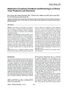
Since the results calculated by Eqs. (15) and (16) are used in the search for maximum values, caution is required when performing calculations for all m except the common proportionality constant component. The speed component associated with the particles selected as having xkMAP is used as v kMAP . The simulation conditions are defined below. First, the initial-period KF error matrix and the covariance matrix are set using σs and σo . The initial value of the KF estimate is 𝟎. The particle number of the PF is set to 1000, and the particles are distributed over a set range as initial values. For this reason, a uniform random variable on x0(m) ∈ [−3, 3] is provided, and v 0(m) = 0 is given under the assumption of no speed. The initial weighting is specified as = 1∕M(±m). The threshold value of ESS used for reπ(m) 0 initialization is set experimentally as 𝐸𝑆𝑆 th = 15 so that the particles can be thoroughly distributed over the range in which the observed noise is generated. Figure 2 shows the time evolution of the state estimate obtained by a simulation in which the position and velocity were estimated by the computations described above for a KF and PF under the above conditions. It can be seen that the transition of the estimated state ((a) in the figure) and the transitions of the estimated error ((b) and (c) in the figure) are virtually the same for the KF and PF. Furthermore, Table 1 shows that the mean squared error (MSE) due to the PF is lower than that of the KF, and that the PF estimate is more accurate than the KF estimate. In addition, it can be seen that the PF estimate converges more quickly up to about the first ten steps.
4.1.2
(b) Esimation error of the position
(c) Esimation error of the velocity
Fig. 2. Time evolution of estimation. The probability distribution of the measurement noise follows a Gaussian distribution. [Color figure can be viewed in the online issue, which is available at wileyonlinelibrary.com.] Table 1. MSE of state values estimated by Kalman and particle filters Filter Kalman filter Particle filter
MSE of position
MSE of velocity
0.089369 0.081069
0.011904 0.011333
(2) In the a-priori scheme the two sensors have identical measurement performance. The observer is designed on the basis of this prior knowledge. (3) In practice, bias and noise with a variance greater than the prior knowledge are included.
Use of two observations
Next, a simulation was performed using two mutually independent observation signals under the following problem formulation:
When using prior knowledge that noise with a probability distribution similar to that of no bias of the two sensors is present, the variance of the probability distribution is reduced by combining the observations based on the two
(1) To improve fault tolerance and observation accuracy, two sensors are provided. The observer performs the state estimations using the two redundant sensors.
19
below, and the two observations can be combined. p
(
y1k , y2k |xk(m)
)
)2 ⎫ ⎧ ( (m) ⎪ xk − y1k ⎪ ∝ exp ⎨− ⎬ 2σ20 ⎪ ⎪ ⎩ ⎭ )2 ⎫ ⎧ ( (m) ⎪ xk − y2k ⎪ + exp ⎨− ⎬. 2σ20 ⎪ ⎪ ⎭ ⎩
Fig. 3. State estimation when measurement noise follows two Gaussian distributions. [Color figure can be viewed in the online issue, which is available at wileyonlinelibrary.com.]
(21)
Using this equation, pf-MAP estimation can be performed as shown below: ) ( xkMAP = argmax p y1k , y2k |xk(m) (m)
xk
sensors, so that the observation accuracy can be increased. However, if an unexpected bias and a large variance occur in one of the sensor signals, the probability density when combining the two sensor signals becomes multimodal and the probability also drops. The concept of the synthesis of the observed noise can be represented by Fig. 3. In order to simulate the above formulation, an observation model different from Eq. (10) used for the simulation described above was created. Observations were performed using the same two sensors, and use was made of prior knowledge that noise with the same probability distributions was combined in the signals. Based on this prior knowledge, the following two observation models shown below were supplied: ( ) (17) y1k = [1 0]x k + ζ1k , ζ1k ∼ b1 , σ21o ( ) ζ2k ∼ b2 , σ22o .
y2k = [1 0]x k + ζ2k ,
⋅
b1 = b2 = 0.
) ( (i) is performed in the same The calculation of p x (m) |x k k−1 way as in Eq. (16). Figure 4 shows the results of state estimations using the KF and PF in accordance with the conditions and procedures given above. It can be clearly seen that bias and noise with a large variance have been added to the second sensor, and that bias from the true state occurs in the KF estimates due to its effects. But the PF estimation is performed as accurately as in the simulation described above. Furthermore, Figs. 4(b) and (c), which show an expanded view of the estimation error for each sate, make it clear that the noise generated in the position estimation by the KF and the velocity estimation accuracy are the same in the KF and PF. These results show that the KF has the property of estimating the median of a multimodal probability density function, and that the PF appropriately extracts the maximum likelihood value of a multimodal probability density function.
(18)
(19)
However, in the simulation, probabilistic noise with a bias and variance different from that of the first sensor is included in the observations of the second sensor: b2 = 1.0,
σ22o = 0.1.
(22)
i=1
Here, the prior knowledge used by the KF and PF is σ21o = σ22o = 0.05,
M ) ( ∑ (i) π(m) p xk(m) |xk−1 . k−1
4.2
Stability due to state feedback control
The following state feedback control system was created to verify the control performance when the KF or PF is used as an observer: [ 2] [ ] [ ] Δ 1 Δ ξ x + 2 u k−1 + 1k (23) xk = 0 1 k−1 ξ Δ 2k
(20)
Next, the procedures by which the KF and PF process the two observed signals in one sampling increment are given. First, KF estimation based on the two observations is performed by the procedure (1) prediction → (2) updating using y1k → (3) prediction → (4) update using y2k → (5) output of state estimate x̂ k .4 The PF performs the likelihood calculations in the fourth line of Algorithm 1 as shown There is no effect on KF estimation if the reference order of y1k and y2k is reversed.
4
20
y1k = [1 0]x k + ζ1k
(24)
y2k = [1 0]x k + ζ2k
(25)
u k = −f T x̂ k
(26)
(a) Time evolution of the position with poles [0.8, 0.8]
(a) True, measurement, and estimated positions
(b) Time evolution of the input with poles [0.8, 0.8]
(c) Time evolution of the position with poles [0.5, 0.5]
(b) Esimation error of the position ( x k − xˆ k )
(d) Time evolution of the position with poles [0.5, 0.5]
Fig. 5. Time evolution of state feedback control. The probability distribution of the measurement noise follows a Gaussian distribution. [Color figure can be viewed in the online issue, which is available at wileyonlinelibrary.com.]
(c) Esimation error of the velocity ( v k − vˆ k )
Fig. 4. Time evolution of estimation. The probability distribution of the measurement noise follows two Gaussian distributions. [Color figure can be viewed in the online issue, which is available at wileyonlinelibrary.com.]
evolution of the control input in Figs. 6(c) and (d) indicates that the fluctuations in the input of the control system using the PF are relatively large compared to those of the KF, and that the PF estimates are slightly more sensitive to observation noise than is the PF estimates, regardless of the pole arrangement.
where x̂ k is the state estimation vector of the KF or PF. The various conditions are the same as in the simulations described above.
4.2.2 4.2.1
Use of two observations
Next, to verify the control performance when observation noise with a multimodal probability distribution is used, Eqs. (24) and (25) were used as the observation model. The conditions were the same as given in Section 4.1.2. Figure 6 shows the time evolution of the control input and output when a pole of the state feedback control system is set at [0.7, 0.7]. First, the results in Fig. 6(a) show that a steady-state deviation occurs in the control results based on the KF estimation. The reason is that the KF estimate converges to a value intermediate between the two observations, as was the case in the simulations described above,
Use of one observation
First, to verify the control performance when using one observation, an observation model using only Eq. (24) was set up. Specifically, unimodal Gaussian noise was introduced into the observation. Figure 5 shows the time evolution of the output and control input when poles of the state feedback control system are set at [0.8, 0.8] and [0.5, 0.5]. Figures 6(a) and (b) show that the state estimates based on the PF and KF and the control results obtained by using them are approximately equal. However, the time
21
Table 2. Relationship between computation time, estimation accuracy, and calculation method of particle filter Condition Nomal Without ESS MMSE MaxMAP
(a) time evolution of the estimated position by KF
Estimation error
0.020405 0.018884 0.000771 0.000762
0.107029 0.128374 0.131110 0.220676
out the use the pf-MAP estimation and the ESS method, under the simulation conditions given in Section 4.2.2. Table 2 provides the results. The notations in the table are as follows: “normal” refers to conditions that are the same as in the simulations given above; “without ESS” refers to the results when resampling is performed in each step without using the ESS method; “MMSE” refers to the results the a-posteriori probability is derived using Eq. (3); “maxMAP” refers to the use of the particles with the greatest weights as represent the MAP estimates. In particular, because “MMSE” is the same as the condition of use of the PF in earlier investigations [8–10], the control results obtained by its use can be understood as the control results for the PF used in earlier investigations. The table shows the average calculation time for each sampling increment, and the average estimation error over a 500 samples under these conditions. The computer OS was Vine Linux 6.1, running on an Intel Xeon E5-02630 (2.3 GHz) CPU with 4 GB of memory. The results show that although the calculation time of the proposed method is long, it has the highest estimation accuracy.
(b) time evolution of the estimated position by PF
(c) time evolution of the inputs
Fig. 6. Time evolution of state feedback control using poles [0.7, 0.7]. The probability distribution of the measurement noise follows two Gaussian distributions. [Color figure can be viewed in the online issue, which is available at wileyonlinelibrary.com.]
due to the bias in the observation noise in the second sensor. The results in Fig. 6(b) show that a no steady-state deviation occurs in the control results based on the PF estimation, and that generally provides good control performance. This is because the PF state estimation is based on the observations in the first sensor, which have small variance. Figure 6(c) shows that although a large control input is needed in the first few steps in the control system using the KF, the subsequent time evolution is roughly the same as in the PF. These results show that state estimation based on the proposed method is more effective than KF-based state feedback control in a control system with multimodal probabilistic noise.
4.3
Calculation time (s)
4.4
Computational load
In discrete system estimation, the selection of the sampling period is often pointed out as an important issue. It has been shown that there is an appropriate sampling period for system parameter estimation, and that good estimation accuracy cannot be obtained if the period is too long or too short [16]. In general, selection of the appropriate sampling period is performed by trial and error based on the time constant of the discrete system and the objective of estimation [16], and the situation is essentially the same under the present method using a PF. However, the estimation procedure using the PF must be repeated in each sampling period, and thus setting a short sampling period is directly linked to an increased computational load. Therefore, the shortest sampling period that a computer running the present method must be estimated, and the best sampling period at that level or higher must be selected. Thus, based on the simulation conditions given in Section
PF calculation method
This paper has introduced resampling decisionmaking based on the ESS method and maximum aposteriori probability estimation method using pf-MAP estimation into the PF calculation procedure. In order to investigate how much these additions contribute to improved estimation accuracy, a simulation was performed in which the estimation accuracy of the PF was determined with-
22
order to avoid the loss of orders of magnitude in the inverse matrix computations when prolonged continuous execution is required for the implementation [18]. In this case, the computational load of the KF is much smaller than that of a PF. However, in lower order systems, such as those in the simulations described above, sufficiently fast execution without problems was possible with both the PF and the KF, even when running C language programs on ordinary computers any particular provision for acceleration. The problem of computational speed can be resolved even when the PF is incorporated into state feedback control in a higher order system [19].
Fig. 7. Relationship between estimation accuracy, calculation time, and number of particles. [Color figure can be viewed in the online issue, which is available at wileyonlinelibrary.com.]
5.
Conclusions
This paper has proposed a method of using a PF as an observer in a state feedback control system. It was explained that in the pole arrangement of a state feedback system, no consideration of convergence speed is needed for PF estimation by the present method, and that the closed loop of the regulator should be designed to be asymptotically stable. Simulations were performed to verify the state estimation performance by means of KF and PF in a state feedback control system based on the proposed method and a free system. The results showed that when unimodal observation noise was added, the KF and PF had similar performance, and that when observations with a multimodal probability density were added, the proposed method achieved more accurate and more stable state estimation than the KF, thus contributing to more accurate control. The results of simulations verified the relationship between the number of particles in the PF, the computational load, and the estimation accuracy, and demonstrated the benefits of the pf-MAP and ESS method introduced above. It was also shown that state estimation robust to lowlevel control systems with non-Gaussian probabilistic noise could be performed using an observer based on the present method. Future work will include application of the present method to more practical examples, and verification of its operation and effectiveness. In particular, extension of the method by the use of an RBPF is essential for its use in higher order systems with four or more dimensions. The development of specific means for using the present method in such cases and verification of its effectiveness will be necessary.
4.2.2, Fig. 6 shows the relationship between the number of particles, the calculation time, and the estimation accuracy. The conditions of the computer used here were the same as those in Section 4.3. First, when the number of particles in the PF was set to 50, the calculation time was an average of 1.0 × 10⁻⁶ s per sample, while for a KF, even with a large mean error of 0.45, an average of 1.9 × 10⁻⁵ s was required for the estimation calculations. The calculation time increased exponentially as the number of particles in the PF rose. In this simulation, no significant difference in estimation accuracy was found at a particle numbers greater than 300. Thus, we see that the estimation accuracy in the presence of multimodal probabilistic noise is lower in the KF than in the PF, the computational load is much lower and computation is faster, and that the number of particles in the PF does not contribute to improved estimation when the number is above some level. In general, the computational load is greater in PFs than in KFs due to the parallel handling of large numbers of particles, and there are many practical problems. Furthermore, the computational load increases exponentially as the number of dimensions rises in a PF [3], and thus, when dealing with higher dimensional systems, it is essential to use a method that represents a causal relations of some of the state variables: the “Rao-Blackwellized particle filter” (RFPF) [2]. In this method, a part in which the state vector is treated as a nonlinear system and a part in which it is treated as a linear system are created. By using a PF only in the former and attaching the estimation of the latter to the estimation for the former either analytically or by using a KF, an increase in the dimension of the KF can be avoided. This technique is called Rao-Blackwellization [17], and the way in which the state vector is divided varies with the plant and estimation objectives. In the KF an SVD may be used in
REFERENCES 1. Doucet A, Freitas N, Gordon N, eds. Sequential Monte Carlo Methods in Practice. pp. 3–14, Springer, New York, 2001.
23
2. Ikoma T. 21st Century Statistical Science III. In Kunitomo, N. ed., pp. 305–338, University of Tokyo Press, Tokyo, 2008. 3. Thrun S, Burgard W, Fox D. Probabilistic Robots. MIT Press, 2005. 4. Ueda R. Evolving probabilistic robots. J Rob Soc Jpn 2011;29(5):404–407. (in Japanese) 5. Driessen JN, Boers Y. Particle filter MAP estimation in dynamical systems. The IET Seminar on Target Tracking and Data Fusion Algorithms and Applications, pp. 1–25, Birmingham, UK, 2008. 6. Godsill S, Doucet A, West M. Maximum a posteriori sequence estimation using Monte Carlo particle filters. The Institute of Statistical Mathematics 2001;53(1):82–96. 7. Saha S, Mandal PK, Bagchi A. A new approach to particle based smoothed marginal MAP. Proc. EUSIPCO, pp. 25–29, 2008. 8. Rigatose GG. Particle and Kalman filtering for state estimation and control of DC motors. ISA Trans 2009;48:62–72. 9. Rigatose GG. Extended Kalman and particle filtering for sensor fusion in motion control of mobile robots. Math Comput Simul 2010;81:590–607. 10. Stahl D, Hauth J. PF-MPC: Particle filter-model predictive control. Systems Control Lett 2011;60:632– 643. 11. Liu JS, Chen R. Sequential Monte Carlo methods for dynamic systems. J Amer Stat Assoc 1998;93(443):1032–1044. 12. Zhou SK, Chellappa R, Moghaddam B. Visual tracking and recognition using appearance: Adaptive models in particle filters. IEEE Trans Image Process 2004;13(11):1491–1506. 13. Candy JV. Bootstrap particle filtering. IEEE Signal Process Mag 2007;24(4):73–85. 14. Boers Y, Driessen JN. A particle filter based detection schemes. IEEE Signal Process Lett 2003;10(10):300– 302. 15. Silverman B. Density Estimation for Statistics and Data Analysis. Chapman and Hall/CRC, Boca Raton, FL, 1986. 16. Aiyo S, Eguchi S. Signal processing in system identification. Meas Control 1989;4(28):309–315. 17. Doucet A, Godsill S, Andrieu C. On sequential Monte Carlo sampling methods for Bayesian filtering. Stat Comput 2000;10:197–208. 18. Katayama T. Applied Kalman Filters, pp. 182–186, Asakura Press, 2000. 19. Ikoma N, Asahara A. Real time color object tracking on cell broadband engine using particle filters. J Adv Comput Intel Intel Inf 2010;14(3):272–280.
20. Capp´e O, Godsill SJ, Moulines E. An overview of existing methods and recent advances in sequential Monte Carlo. IEEE Proc 2007;95(5):899–924.
Appendix A A Derivation of pf-MAP The MAP estimation for the probability density filtered at time k is given as follows: MAP = argmax p(xk |y1∶k ). xk|k xk
(A1)
Using the PF, the a posteriori probability density with respect to a general nonlinear model can be approximated as follows using a weighted particle group of M elements: P̂(dxk |y1∶k ) ≃
M ∑ i=1
πk(i) δx (i) (dxk ). k
(A2)
Applying the Bayes Rule, a posteriori probability density function (A.1) can be expressed as follows: p(yk |xk ) p(xk |y1∶k−1 ) p(x|y1∶k ) = (A3) p(yk |y1∶k−1 ) where the denominator is independent of x k . Thus ( ) ( ) p(x |y 1∶k ) ∝ p y k |x k p x k |y 1∶k−1 (A4) can be used, and in (A-1) can be expressed as ( ) ( ) xkMAP = argmax p y k |x k p x k |y 1∶k−1 . xk
(A5)
The likelihood p(y k |x k ) can be calculated for all x k , and thus the main problem in deriving the equation above is to calculate the expected probability density function p(x k |y 1∶k−1 ). Thus the following relation can be used: p(xk |y1∶k−1 ) =
∫
p(xk |xk−1 ) p(xk−1 |y1∶k−1 )dxk−1 . (A6)
Furthermore, in accordance with Eq. (A2), an approximation of p(x k |y 1∶k−1 ) can be obtained by using Monte Carlo integration: p(xk |y1∶k−1 ) ≃
M ) ( ∑ (i) (i) πk−1 p xk |xk−1 .
(A7)
i=1
By substituting Eq. (A7) into Eq. (A4), the MAP estimate (pf-MAP) is derived as follows: M )∑ ) ( ( (i) π(m) xkMAP = argmax p yk |xk(m) p xk(m) |xk−1 . k−1 (m)
xk
i=1
(A8) The computational load is O(M 2 ).
24
AUTHOR
Takeshi Nishida (member) received a bachelor’s degree in design and manufacturing engineering from Kyushu Institute of Technology in 1998. He completed the latter half of the doctoral program at the Graduate School of Engineering of the same university in 2002 and became a research associate in the Faculty of Machine Intelligence. He became an assistant professor in 2007. He holds a D.Eng. degree. He is engaged in research on outdoor mobile robots. He is a member of the Robotics Society of Japan, SICE, the Japan Neural Network Society, and IEICE.
25