Revision for J. of the Air and Waste Management Association, dated April 7, 2000. Contact:
[email protected].
STATE-SPACE MODELING OF THE RELATIONSHIP BETWEEN AIR QUALITY AND MORTALITY
Murray, Christian J., Department of Economics, University of Houston, Houston, Texas Nelson, Charles R., Department of Economics, University of Washington, Seattle, Washington
Copyright 2000 by Christian J. Murray and Charles R. Nelson Not to be quoted without authors’ permission.
IMPLICATIONS Mortality in an at-risk population may be modeled in a state-space framework. The relation of the hazard rate to particulates (TSP) and other variables and the unobserved population are estimated using the Kalman Filter and maximum likelihood. The results for daily data from Philadelphia suggest that both TSP and temperature are risk factors, the effect of both rising at high temperature levels. The appropriate metric for health damage is the effect of particulates on life expectancy, which in the context of daily variation is estimated to be on the order of days.
ABSTRACT A portion of a population is assumed to be at-risk, mortality hazard varying with atmospheric conditions including total suspended particulates (TSP). This at-risk population is not observed
and the hazard function is unknown; we wish to estimate these from mortality count and atmospheric variables. Consideration of population dynamics leads to a state-space representation, allowing the Kalman Filter to be used for estimation. An implication is that there is a harvesting effect; high mortality is followed by lower mortality until the population is replenished by new arrivals.
The model is applied to daily data for Philadelphia, 1973-90. The estimated hazard function rises with the level of TSP and at the extremes of temperature and also reflects a positive interaction between TSP and temperature. The estimated at-risk population averages about 480 and varies seasonally. We find that lags of TSP are statistically significant, but the presence of negative coefficients suggests their role may be partially statistical rather than biological. In the population dynamics framework, the natural metric for health damage from air pollution is its impact on life expectancy. The range of hazard rates over the sample period is 0.07 to 0.085, corresponding to life expectancies of 14.3 and 11.8 days respectively.
INTRODUCTION An extensive literature documents evidence that episodes of severe air pollution are associated with heightened mortality in urban populations. However, the question of whether mortality occurs within a relatively limited population of frail individuals, or whether the risks are more diffuse across the general population, has a long history and is still being examined and debated by researchers.1,2,3
2
In this paper, we explore a new approach to modeling the relationship between mortality and air quality and apply it to daily data from Philadelphia. We take as given that a portion of the urban population is at-risk, being subject to a probability of death, or hazard rate, that varies with atmospheric conditions including total suspended particulates (TSP). New entrants replenish the at-risk population over time. Only mortality and atmospheric conditions are observed, the at-risk population, new entrants, and the hazard rate being unobserved. Because of the dependence of mortality on the unobserved at-risk population, the model is not directly estimable as a regression, but fortunately it may be cast in state-space form. Using the Kalman Filter (KF) we then infer the hazard rate over time, its relationship to atmospheric variables, and the implied path of the unobserved at-risk population. In the state-space framework one is able to address the following questions. What is the size of the at-risk population? What is the life expectancy of individuals in that population? What is the effect of changes in air quality on that life expectancy?
The implications of the at-risk population model in state-space form differ fundamentally from those of linear models based on multiple regression.4 In the latter, a risk factor such as TSP affects mortality directly and a persistent rise in the level of TSP would imply a persistent rise in mortality count. In the state-space model the impact of a risk factor such as TSP on mortality is indirect; it is proportional to the size of the at-risk population on that day which is not observed directly. If the at-risk population has been depleted by recent mortality, then the impact of risk factors will be mitigated since it is a temporarily smaller population that is at risk. Indeed, it is this “harvesting effect” which allows the unobserved at-risk population to be estimated by the KF. If the higher hazard rate persists, the mortality count will fall back towards its previous
3
level, since in the long run mortality is limited to the rate of new arrivals. However, the life expectancy of those in the at-risk population will fall and this paper presents estimates of that effect.
MODEL SPECIFICATION AND ESTIMATION Any population is diminished by deaths and replenished by the arrival of new entrants; in this case the population of individuals in Philadelphia who are at risk from changing air quality. Using Pt to denote the number of individuals in the at-risk population at the end of day t, Dt the number of deaths (mortality) during day t, and Nt the number of new entrants to the at-risk population during day t, the basic equation of population dynamics is:
Pt = Pt − 1 + N t − Dt .
(1)
Equation (1) may be viewed as simply an accounting relation that states that the at-risk population at time t is equal to its previous value plus the number of new entrants less the number of deaths. The only variable in this relationship that is actually observed in the present context is the mortality count.
Mortality is influenced by atmospheric variables through a hazard function that operates on the at-risk population. Listing atmospheric variables in a vector denoted xt, we assume the hazard function to be the linear combination of these variables, denoted (γ ′ xt). The atmospheric variables listed in xt will include measures of air pollution such as TSP and weather variables such as
4
average temperature (AVGT). The elements of the vector γare coefficients that indicate how each atmospheric variable affects the hazard function. These coefficients are unknown and will have to be estimated from data. The hazard rate is the value of the hazard function at period t and it is the expected fraction of deaths in the at-risk population on that date. Some deaths will result from other factors that affect mortality but which we have not included in xt so there will also be an error term, denoted et, which is the difference between actual and expected mortality.
We summarize this discussion by the expression:
Dt = (γ' x t )•Pt − 1 + et .
(2)
A constant in the hazard function captures the average level of mortality, so the mean value of the error term is zero. We seek to estimate the γvector of coefficients and the time series of the unobserved at-risk population P from daily data on mortality and atmospheric variables.
Note that equation (2) implies that mortality is a nonlinear function of Pt-1 and the atmospheric variables, the expected number of deaths being the product of hazard and population. This implies that mortality cannot be expressed as a linear function of current and past atmospheric variables with constant coefficients. Indeed, the response of mortality to a change in atmospheric conditions depends on the time path of past conditions, reflected in the current level of the at-risk population.
5
To complete the model we need to say how Nt, the unobserved number of new entrants to the at-risk population, evolves through time. In any population, it is the rate of arrival of new entrants that determines mortality over a long time span. The time series of mortality of those over 65 in Philadelphia displays remarkably little long-term variation over the fourteen-year period of our sample. The annual averages fluctuate in a narrow range around the long run average of 35, ranging from 33 to 37, and ending the period at the upper end of that range. Further, Dickey-Fuller tests strongly reject non-stationarity or drift over long time horizons. Given the long run relationship between arrivals and mortality, these all suggest that the rate of arrivals fluctuates around a long run mean during this period in the Philadelphia population. With this background, we employ the specification
N t = N + ηt ,
(3)
where N is the average number of arrivals, and ηt is a random deviation.
The fundamental problem of statistical inference in this setting is that the at-risk population is an unobserved variable. If Pt-1 were observed then one could estimate (2) by least squares, regressing mortality on variables that would be cross-products of the x’s and Pt-1. However, Pt-1 is not observed, so the model is non-linear and cannot be expressed as a linear regression. Fortunately, this model is a member of the class of state-space models that can be made operational using the Kalman Filter (KF). Briefly, the state-space representation consists of two equations, a measurement equation and a state equation. The former shows how the variable we observe and wish to explain depends on unobserved variables called state variables. The latter
6
shows how those state variables evolve through time. Thus, equation (2) is the measurement equation and equations (1) are (3) are combined to form the state equation. The random shocks in these two equations are assumed uncorrelated in the state-space formulation. Those shocks are errors in predicting mortality and random arrivals to the at risk population respectively. The assumption that they are uncorrelated is equivalent to saying that there is a well-defined at-risk population in the sense that movement of individuals from the population at large to the at-risk population does not depend on mortality. We want the model to estimate the size of the at-risk population, so we would not want to exclude a portion of the population that is also at risk. Given parameter values, we obtain an estimate of the series Pt by “running” the data through the KF.5,6 The resulting estimated level of Pt, denoted Pt|t, is the minimum mean squared estimate of Pt based on data up to time t and is referred to as the filtered estimate.
A by-product of the KF is the construction of the Gaussian likelihood function using Harvey’s prediction-error decomposition.7,8 Maximum likelihood estimation is carried out using the OPTMUM module of the GAUSS programming language. The prior distribution for the initial value of the unobserved at-risk population was given a mean of 0 and variance 1000, a very loose prior distributions that leaves determination of the at-risk population and to be determined by the data. No prior is required for Nt since it is just a constant plus a random error. Maximum likelihood estimates of the parameters are computed by maximizing the likelihood function over the parameter space. This requires that we assume that the error terms in equations (2) and (3) are Normal, serially random, and uncorrelated with each other as well as with variables in the model. The error terms cannot be exactly Normal in this context since mortality is integer valued and non-negative, so what we have is an approximation to maximum likelihood.
7
Standard errors for parameter estimates are based on asymptotic distribution theory that may not be exact in finite samples, but sample size here is very large. The parameters to be estimated are as follows: the γvector, the average arrival rate N, and the standard deviations of the two error terms e and η denoted σe and ση respectively. The t-statistic shown in parentheses under each point estimate in the tables is based on numerical second derivatives to obtain standard errors. The value of the log of the likelihood function is also reported since it gives us a basis for comparing models using likelihood ratio tests or information criteria. For nested models, the likelihood ratio test is that two times the difference in log likelihood will be approximately chisquare with degrees of freedom equal to the number of additional parameters in the more complex model.
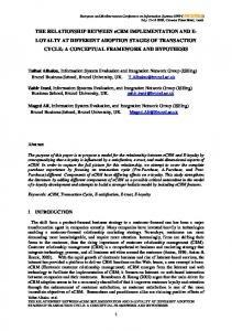
We have verified that the algorithm does in fact uncover the underlying parameters and the at-risk population in a system having the structure of (1) – (3) by confronting it with artificial mortality data that we generated. Our hazard function was (.1 + .003• xt) where the sequence {xt} was constructed to mimic the behavior of TSP in the actual data. N was set at the mean mortality rate in the real data and the standard deviations of the error terms were set at 2 and 3 respectively. Series length was 6000 to be comparable to the daily data we study. To increase the validity of the experiment, one of us generated the data, providing the other with only the mortality and TSP series to carry out the estimation. The parameter values were estimated correctly to within very small tolerances. The accuracy of estimates of the unobserved population is apparent in Figure 1 where the generated “actual” population is plotted along with the KF estimates of population over an arbitrary sequence of 400 days. The latter tracks both the local trend and day-to-day fluctuations. The Kalman filter requires a prior distribution for the
8
unobserved state variable Pt at t=0. The results were not sensitive to modifications of this prior. We found that the estimated Pt moved very quickly from its initial guess value to the correct level. These results give us added confidence in the validity of our results.
RESULTS FOR THE PHILADELPHIA MORTALITY DATA We apply the model to daily data for Philadelphia from the period 1973-90 provided to us by the Electric Power Research Institute. The data set includes daily observations on the number of non-accident deaths of individuals over age 65, a measure of total suspended particulates (TSP), and other atmospheric variables including temperature, barometric pressure, and ozone. Our investigation focused on the relationship of mortality to TSP. Before we were able to estimate the model, we had to address the problem of missing-observations in the TSP series. Eliminating periods at the beginning and end of the sample where there are large gaps in the TSP record leaves a sequence of 5136 consecutive days within which there are only 50 days missing TSP values. To fill in these gaps we regressed TSP on other atmospheric variables, using the integer part of the fitted series.
Table 1 displays Maximum Likelihood estimates of the observation and state equations for six base-line specifications of the x vector that include various combinations of TSP and average temperature (AVGT), the square of temperature, and the multiplicative interaction of temperature with TSP. We chose AVGT as a baseline variable because of its strong linear association with daily mortality. A constant term is included in every case. Model 1 uses only TSP, which is highly significant. Model 2 adds AVGT, which is also highly significant. Model 3 adds the square of AVGT to allow for a hazard rate that increases at both extremes of
9
temperature, and that effect is also significant. Model 4 allows the effect of TSP and AVGT to each depend on the value of the other by adding the interaction variable AVGT*TSP. That interaction is significant, while TSP and AVGT alone are much less significant than in Model 3. Model 5 is included for comparison purposes and uses only the AVGT variables. Model 5 has roughly the same log likelihood as Model 1 which used only TSP. Finally, Model 6 uses all of the variable considered in this table: TSP and AVGT, the square of AVGT, and the interaction AVGT*TSP.
How important is TSP as a predictor of mortality? Comparing the log likelihood for Model 6 with that of Model 5 that does not include either TSP-related variable, the difference in value is about 14 which is highly significant (p-value is off the chi-square table). How important are the temperature-related variables? Comparing Model 6 with Model 1 the difference in log likelihoods is again about 14, and even with 3 additional parameters that difference is overwhelmingly significant. We also note that although the interaction variable AVGT*TSP has a t-statistic of only 1.42 in Model 6, when we compare the log likelihood with that of Model 3, the difference is about 2. That corresponds to a p-value of about .05, supporting a role for the interaction term. Thus, we regard Model 6 as a reasonable baseline specification. Note that to interpret the effect of TSP on the hazard rate in Model 6 one needs to keep in mind that the coefficient of TSP is a linear function of AVGT, so the effect is positive in spite of the negative coefficient of TSP by itself. We also note that the residuals in the state equation lack serial correlation as assumed. For Model 6, those residuals display serial correlation of -.012 at lag one day, -.019 at lag 7 days, and .026 at lag 365 days and none is statistically significant.
10
How do TSP and temperature affect the hazard rate? The hazard function of Model 6 implies that both extremes of temperature are harmful, and that TSP is also harmful with that effect rising with temperature. At a typical level of TSP, the effect of an increase in temperature from 40F to 90F is an increase in the hazard rate from .07 to .08. At a high temperature of 90F, the effect of an increase in TSP from zero to the highest levels observed in the sample it to raise the hazard rate from .075 to .091. Any statements about the effect of TSP on the hazard rate need to be tempered by the uncertainty connected with these estimates.
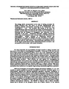
Figure 2 plots the KF estimate of the at-risk population and the estimated hazard rate in Model 6. The estimated at-risk population averages 484, and varies seasonally. Since average mortality is 35 per day, this implies that about 7% of the at-risk population dies on average per day. The corresponding time series of the hazard rate in Figure 2 is stable around its mean of .073, remaining well within the required (0,1) interval for a probability. The hazard rate fluctuates seasonally as periods of high TSP and temperature extremes reap a grim harvest, followed by less lethal conditions. As noted above, the mortality series is essentially trendless, so it is of some interest that the estimated at-risk population series does move higher with time, from an annual average of around 470 in early years to around 500 at the end. There is a corresponding and offsetting decline in the hazard rate, moving downward from an annual average of about .072 in early years to .0716 in later years. This decline in the hazard rate is driven by declining TSP over the period; from annual averages of about 80 to about 70, the result of efforts to clean up the air around Philadelphia. A lower hazard rate lengthens life expectancy, and allows individuals to stay longer in the at-risk population, thereby making that population
11
larger. Finally, we note that output from all six models is qualitatively similar in producing population and hazard rate estimates that are stable and positive.
Does TSP have a cumulative effect on mortality over several days? We investigated this possibility by adding the level of TSP in preceding days to the list of variables in the hazard function in Models 1 through 3. The results for adding 4 or 8 lags of TSP are displayed in Table 2 which differs from Table 1 in adding another line listing the likelihood ratio statistic for testing the null hypothesis that all the added lagged values of TSP have a zero coefficient. What the test results indicate is that lags of TSP do have explanatory power that is statistically significant, but the coefficient estimates suggest that the effect is not large. The coefficient of current day TSP is reduced when lags are added, the first lag is positive and significant, but the second lag is negative and remaining lags have small estimated coefficients. The sum of all TSP coefficients for Model 3 is raised, however, by almost half when 8 lags are added. How do we understand a negative effect of TSP after two days? One explanation is that the apparent effect of lags of TSP is partially statistical rather than biological. If we measure TSP imperfectly, due to aggregation over the 24-hour day or extrapolation of atmospheric measurements across a geographical region, then TSP on adjacent days may contain additional information relevant to the explanation of mortality. The lag pattern we obtain then may represent, at least in part, a kind of moving average measure of TSP rather than a biological process. Both factors may well be at work in producing the pattern seen here.
We have also experimented with adding other atmospheric variables to base-line Model 6. Barometric pressure on the same day enters the model with a negative and significant coefficient
12
while the coefficients on TSP and AVGT change only slightly. The resulting estimated population and hazard series are essentially indistinguishable from those of Model 6.
DISCUSSION AND CONCLUSIONS In thinking about the dynamics of the state-space model we have found it useful to compare it to the more familiar linear regression or distributed lag model linking mortality to risk factors. The latter have the form
Dt = α +
K
∑β k =0
k
x t − k + εt .
(4)
The impact of xt-k on mortality is given by fixed coefficients in (4), while in the state-space model the impact depends on the unobserved state variable P. Because this functional relationship is multiplicative, the state-space model is highly non-linear. In particular, the impact will be smaller if recent mortality has been high, since the at-risk population will have been reduced. This harvesting effect is small in the models we estimated, but it is very persistent since the rate of replenishment of the population by new arrivals is slow. Thus, the relation of past atmospheric conditions to mortality is highly non-linear in the state-space model.
If we nevertheless run regressions of the form of (4) on the Philadelphia data set with TSP as the risk factor there is a consistent pattern in the coefficients obtained. For example, with lags up to seven days the lag zero coefficient is .013, but the sum over lags zero through 7 days is -.041. The character of the results is not sensitive to including more lags and other variables; the leading coefficient on TSP is positive but the sum 13
∑β
k
is small or negative. Thus, a positive
association between mortality and TSP on the same day is more than offset by a sequence of negative coefficients, as predicted by the harvesting effect. The state-space model also predicts that the sum of coefficients will be small, since over the long run the level of mortality is only determined by the rate of arrivals, not by risk factors. Thus the state-space model proposed here helps explain why multiple regression produces results that are otherwise hard to explain, namely an apparent negative effect of TSP on mortality after a lag. While an increase in risk factors cannot increase mortality in the long run, life expectancy is the inverse of the hazard rate, so hazard-causing agents will shorten it. The range of hazard rates observed in our sample over the sample period is roughly 0.07 to 0.085. Since life expectancy is the reciprocal of the hazard rate, the former corresponds to a life expectancy in the at-risk population of 14.3 days, while the latter to 11.8 days, a difference of about 2.5 days on average for the roughly 500 individuals at-risk in Philadelphia. In summary, we feel that the state-space approach represents a very promising avenue of research in modeling the effects of air pollution. Its primary advantage comes from explicit recognition of the role of population dynamics in mortality, and making use of the Kalman Filter to estimate the population model directly. The results reported here are preliminary, but suggest that the approach is practical and provides explanations of otherwise puzzling results from conventional analysis.
14
Table 1. Parameter Estimates for Baseline State-Space Models, Philadelphia Data. Coefficient
Model 1
Model 2
Model 3
Model 4
Model 5
Model 6
1
0.0632924
0.0650052
0.0696869
0.0686944
0.0765619
0.0711416
(8.61)
(9.34)
(8.95)
(7.72)
(8.94)
(1.89)
0.0000534
0.0000480
0.0000412
-0.000023
n.a.
-0.000007
(5.60)
(5.50)
(4.09)
(-0.69)
n.a.
0.0001002
-0.000167
0.0000079
-0.000213
-0.000168
(2.96)
(-2.95)
(0.62)
(-1.88)
(-0.21)
n.a.
0.0000030
n.a.
0.0000041
0.0000023
(3.35)
(0.28)
n.a.
0.0000009
TSP
AVGT
AVGT^2
n.a.
(4.34) AVGT*TSP
n.a.
n.a.
n.a.
0.0000013
(-0.21)
(2.28) σe ση
N
lnL
(1.42)
5.80991
5.756863
5.754371
5.755896
5.731345
5.754223
(76.69)
(74.90)
(74.15)
(73.14)
(73.79)
(49.13)
19.7923
19.04966
19.05996
19.18479
18.58655
19.15221
(13.63)
(14.81)
(13.95)
(13.39)
(14.78)
(5.96)
35.0947
35.08667
35.08826
35.08771
35.08178
35.08867
(126.84)
(131.80)
(131.73)
(130.85)
(135.08)
(131.02)
-16924.9
-16919.03
-16913.12
-16914.00
-16924.72
-16910.97
Note: t-statistics for the null hypothesis that an individual coefficient is zero are in parentheses beneath it. The statistic lnL is the log of the likelihood function.
15
Table 2. Parameter Estimates for State-Space Models with Lags of TSP, Philadelphia Data. Coefficient 1
Model 1a 0.061616 (8.62) 0.000043 (4.64) 0.000034 (4.11) -0.000011 (n.a.) 0.000009 (2.26) 0.000007 (3.20) n.a.
Model 1b 0.057272 (8.30) 0.000042 (1.62) 0.000033 (0.94) -0.000011 (-0.22) 0.000009 (0.51) 0.000004 (0.41) 0.000005 (0.39) 0.000010 (1.26) -0.000006 (-0.68) 0.000000 (0.01) n.a.
Model 2a 0.063138 (9.86) 0.000040 (4.76) 0.000030 (3.73) -0.000013 (n.a.) 0.000009 (6.11) 0.000005 (n.a.) n.a.
Model 2b 0.058708 (8.76) 0.000040 (4.43) 0.000030 (3.18) -0.000013 (-4.51) 0.000008 (n.a.) 0.000002 (0.38) 0.000004 (0.68) 0.000010 (1.58) -0.000006 (-1.31) -0.000000 (0.05) 0.000058 (1.22) n.a.
Model 3a 0.067901 (10.85) 0.000033 (4.31) 0.000028 (3.33) -0.000015 (-2.38) 0.000007 (n.a.) 0.000004 (3.03) n.a.
Model 3b 0.0632121 (16.03) TSP 0.000033 (4.58) TSP(-1) 0.000027 (n.a.) TSP(-2) -0.000014 (n.a.) TSP(-3) 0.000007 (n.a.) TSP(-4) 0.000002 (n.a.) TSP(-5) 0.000004 (n.a.) TSP(-6) n.a. n.a. n.a. 0.000011 (n.a.) TSP(-7) n.a. n.a. n.a. -0.000006 (n.a.) TSP(-8) n.a. n.a. n.a. 0.000000 (n.a.) avgt n.a. 0.000070 -0.000018 -0.000177 (2.58) (0.00) (2.44) avgt^2 n.a. n.a. n.a. 0.000003 0.000003 (3.06) (3.41) 5.80483 5.82535 5.73976 5.79522 5.76622 5.79049 σe (76.22) (79.24) (77.88) (74.44) (78.30) (81.75) 19.5818 20.0188 19.1180 19.5942 19.1418 19.5993 ση (13.79) (13.54) (15.99) (14.15) (16.43) (15.91) N 35.0924 35.0979 35.0866 35.0924 35.0877 35.0935 (128.18) (124.58) (131.30) (128.04) (131.23) (128.01) lnL -16906.7 -16884.9 -16904.1 -16882.8 -16898.6 16877.2 *** *** *** *** *** LR 36.4 80.0 38.4 72.46 29.04 67.54*** Notes: LR is the likelihood ratio statistic for testing the null hypothesis that the coefficients on all lags of TSP are zero; and in each case LR is significant at a p-value below .01. Individual t-statistics are not available in cases where the standard error could not be computed. See also the notes to Table 1.
16
REFERENCES 1. Schimmel, B. Bul. N Y Acad. Of Med. 1978, 54, 1052-1109. 2. Lipfert, F.; Wyzga, R. J. Air Waste Manage. Assoc. 1993, 45, 949-966. 3. Zeger, S. L.; Dominici, F.; Samet, J. Epidemiology 1999, 10, 171-175. 4. Pope, C. A., Schwartz, J., Am. J. Respiratory and Critical Care Medice, 1996, 154, S229S233. 5. Kalman, R. E. Trans ASME J. of Basic Engineering, 1960, D 82, 35-45. 6. Kalman, R. E.; Bucy, R. S. Trans ASME J. of Basic Engineering, 1961, D 83, 95-108. 7. Harvey, A. C., Time Series Models; The MIT Press: Cambridge, 1993, 89-95. 8. Kim, C-J; Nelson, C. R., State Space Models with Regime Switching, The MIT Press: Cambridge, 1999, 19-58.
LIST OF FIGURES Figure 1. Comparison of actual at-risk population and Kalman Filter estimate for simulated data. Figure 2. Estimated Hazard Rate and KF estimate of at-risk population in Model 6.
ABOUT THE AUTHORS Christian J. Murray is Assistant Professor of Economics at the University of Houston (Department of Economics, Houston, TX 77204;
[email protected]). Charles R. Nelson is the Ford and Louisa Van Voorhis Professor of Economics at the University of Washington (Department of Economics, Box 353330, Seattle, WA 98195;
[email protected]). Both authors work in time series econometrics, and have collaborated on papers that investigate the
17
nature of trend and cycle in GDP. They were consultants to the Electric Power Research Institute on this project.
ACKNOWLEDGMENTS This research was supported by the Electric Power Research Institute. We are grateful to Fred Lipfert and Ron Wyzga who provided invaluable information, suggestions, and insights throughout this project. We also received helpful comments from Richard Burnett, Robert Engle, Levis Kochin, Jeremy Piger, Richard Startz, Mark Wohar, and anonymous referees. The views expressed, however, are those of the authors who are solely responsible for the content of this article.
18
160 140 120 100 80 60 40 3050 3100 3150 3200 3250 3300 3350 3400 POP_ACTUAL
POP_ESTIMATE
Figure 1. Comparison of actual at-risk population and Kalman Filter estimate for simulated data.
0.090 0.085 0.080 0.075 800
0.070
600
0.065
400 200 0 1000
2000
3000 POP6
4000
5000
HAZ6
Figure 2. Estimated Hazard Rate and KF estimate of at-risk population in Model 6.
19