Static Friction Experiments and Verification of an

Chul-Hee Lee1 Andreas A. Polycarpou2 e-mail: [email protected] Department of Mechanical Science and Engineering, University of Illinois at Urbana-Champaign, Urbana, IL 61801

Static Friction Experiments and Verification of an Improved Elastic-Plastic Model Including Roughness Effects An experimental study was conducted to measure the static friction coefficient under constant normal load and different interface conditions. These include surface roughness, dwell time, displacement rate, as well as the presence of traces of lubricant and wear debris at the interface. The static friction apparatus includes accurate measurement of friction, normal and lateral forces at the interface (using a high dynamic bandwidth piezoelectric force transducer), as well as precise motion control and measurement of the sliding mass. The experimental results show that dry surfaces are more dependent on the displacement rate prior to sliding inception compared to boundary lubricated surfaces in terms of static friction coefficient. Also, the presence of wear debris, boundary lubrication, and rougher surfaces decrease the static friction coefficient significantly compared to dry smooth surfaces. The experimental measurements under dry unlubricated conditions were subsequently compared to an improved elastic-plastic static friction model, and it was found that the model captures the experimental measurements of dry surfaces well in terms of the surface roughness. 关DOI: 10.1115/1.2768074兴 Keywords: static friction coefficient, model, experimental, elastic-plastic contact, surface roughness

1

Introduction

The need to know the friction values in different engineering applications has been acknowledged for many years, and certainly since Leonardo da Vinci, with his classic illustrations alluding to the friction force dependence on normal load and nominal contact area. During the last two centuries, a significant number of experiments under different conditions have been performed and friction values have been extensively tabulated. However, despite the plethora of experimental friction measurements, two major issues that remain are as follows: 共i兲 specific friction coefficient values appear to be inconsistent when compared from different reported sources and 共ii兲 a basic universally acceptable physics-based friction model applicable to realistic surfaces does not exist in the literature. Typical investigations on static friction report on experimental measurements under different surface conditions and, in some cases, propose friction models, which are usually applicable to a specific interface. For example, Gassenfeit and Soom 关1兴 measured the instantaneous coefficient of friction during start-up at a planar contact under four different lubrication conditions. Polycarpou and Etsion 关2兴 compared a static friction model 共termed subboundary lubrication model兲 with experimental measurements on thin-film magnetic disks. Xie et al. 关3兴 experimentally measured the coefficient of static friction for common workpiece-fixture joints consisting of cast aluminum and iron. Hwang and Zum Gahr 关4兴 evaluated the effect of surface roughness and lubrication on the transitional behavior from static to kinetic friction, and Etsion et al. 关5兴 performed an experimental investigation using a 1 Currently with the Department of Mechanical Engineering, Inha University, Incheon 402-751, Republic of Korea. 2 Corresponding author. Contributed by the Tribology Division of ASME for publication in the JOURNAL OF TRIBOLOGY. Manuscript received January 10, 2006; final manuscript received April 17, 2007. Review conducted by Kwangjin Lee.

754 / Vol. 129, OCTOBER 2007

sphere on flat configuration and measured the decrease of the static friction coefficient with increasing normal loads. Engineering surfaces are not infinitely smooth and possess finite roughness. To account for surface roughness, statistical rough surface contact models have been introduced starting from the classic work of Greenwood and Williamson 关6兴, where they developed a statistical model 共GW model兲 for elastic contacts by assuming that asperities are represented by geometrical spherical shapes and the asperity heights follow a Gaussian probability density function. In order to account for elastic-plastic asperity contacts, Chang et al. 关7兴 developed an elastic-plastic contact model 共CEB model兲, which is an extension of the original GW model, and subsequently used this model to develop a static friction coefficient model for rough surfaces 关8兴. However, the CEB friction model underestimates the static friction coefficient, especially for higher plasticity contact, because it neglects the ability of plastically deformed asperities to resist additional tangential loading. This problem was resolved by Kogut and Etsion 关9兴, where they improved the CEB static friction model by accounting for the resistance to sliding of plastically deformed asperities. Despite the physics-based analytical foundation of this model and its comparison to other models, there has not been an experimental comparison because the model requires specific material and roughness information that are usually not available in the published literature. In this paper, we measured the static friction coefficient between flat, rough contacting surfaces and directly compared it to the Kogut and Etsion 关9兴 static friction model 共KE model兲. Using advanced instrumentation, which includes a closed-loop microactuator and a triaxial piezoelectric force transducer, we were able to obtain detailed static friction measurements under constant normal load and various controlled conditions. The measured roughness, material, and geometrical properties of the samples tested were entered directly into the KE model to predict the static friction coefficient values, which were compared to the experimental friction results.

Copyright © 2007 by ASME

Transactions of the ASME

Downloaded 19 Sep 2007 to 130.126.178.167. Redistribution subject to ASME license or copyright, see http://www.asme.org/terms/Terms_Use.cfm

Fig. 1 Schematic of a typical friction coefficient showing static and kinetic friction

2

Static Friction Model

A typical friction transition in contacting solid bodies under unlubricated dry conditions and constant normal load is depicted as static friction coefficient being higher than kinetic friction coefficient, as shown schematically in Fig. 1. Considering the stochastic nature of surface interactions between flat sample surfaces, a static rough surface contact model can be used to theoretically calculate the static friction coefficient and compare it to measured values. In order to use this statistical model, the two rough surfaces in contact are replaced with a single equivalent rough surface in contact with a smooth rigid surface, as shown in Fig. 2.

Figure 2共a兲 shows a typical rough contacting interface with the relevant interfacial forces, where F is the external load, P is the total asperity contact force, Fs is the total adhesive force, and Qmax is the static friction force 共also see Nomenclature兲. In the GW model it is assumed that the asperity heights follow a Gaussian probability distribution with a standard deviation of their heights ␴, their shape is spherical and all have the same radius of curvature R, and the surface has a finite number of these asperities 共areal density ␩兲. Kogut and Etsion 关9兴 used the basis of the GW elastic model to develop an improved elastic-plastic contact, adhesion and friction model for a rough contacting interface under unlubricated conditions. Also, Jackson and Green 关10兴 presented a similar 共to the KE兲 elastic-plastic model, where they used the material’s yield strength instead of hardness, because the hardness is known to change with the evolving contact geometry and material properties, with their normal contact results 共because they do not analyze friction兲 being comparable to the KE model results 关9兴. 2.1 KE Elastic-Plastic Static Friction Model. In the KE model 关9兴, the rough surfaces are modeled as in the GW model shown in Fig. 2共b兲. The contact load is given by 2 P共d*兲 = AnH␲␤K␻*c 3 + 1.4

冕

冋冕

d*+␻c*

I1.5 + 1.03

d*

d*+110␻c*

I1.263 +

d*+6␻c*

3 K

冕

冕

d*+6␻c*

I1.425

d*+␻c*

⬁

I1

d*+110␻c*

册

共1兲

where, the asterisk indicates dimensionless values normalized by ␴, and Ib is a general form of the integrand,

Ib =

冉 冊 z* − d*

b

␾*共z*兲dz*

␻*c

共2兲

Also, the adhesion force is given by

Fs共d*兲 = 2AnH␲␤␪

+ 0.79

冕

冋冕

d*

d*+␻c*

0.298 J−0.29

d*

−⬁

d*+6␻c*

冕 冕

d*+␻c*

Jnc + 0.98

0.356 J−0.321 +

d*+110␻c*

1.19

d*+6␻c*

0.093 J−0.332

册

共3兲

where Jnc and Jbc are general forms of the integrands accounting for the contribution of noncontacting and contacting asperities

Jnc =

4 3

冋冉 冊 ␧* d* − z*

Jbc =

Fig. 2 Contacting nominally flat rough interface: „a… schematic showing relevant interfacial forces, and „b… GW roughness model showing the contact between an equivalent sum rough surface in contact with a smooth plane

Journal of Tribology

冉

2

− 0.25

␧* d* − z*

冉 冊冉 冊 z* − d*

␻*c

b

␧*

␻*c

冊册 8

␾*共z*兲dz*

共4兲

c

␾*共z*兲dz*

共5兲

␧ 共␧* = ␧ / ␴兲 is the equilibrium distance between two surfaces under zero applied load. In this work, it is taken to be 0.158 nm 关11兴, which is the value for iron 共Fe兲, because we have used steel samples. The effect of the equilibrium distance on friction is expected to be small because adhesion is also small, in the cases of “rougher” surfaces considered in this work. This will not be the case for microelectromechanical systems and magnetic storage applications with nanometer roughness. The static friction force can be obtained by OCTOBER 2007, Vol. 129 / 755

Downloaded 19 Sep 2007 to 130.126.178.167. Redistribution subject to ASME license or copyright, see http://www.asme.org/terms/Terms_Use.cfm

Fig. 3 Typical specimens and surface roughness profile „500 ␮m à 500 ␮m… measured using a 3D contact profilometer

冋

2 Qmax共d*兲 = AnH␲␤K␻*c 0.52 3

冕

d*+␻c*

I0.982 +

冕

d*+6␻c*

d*+␻c*

d*

⫻共− 0.01I4.425 + 0.09I3.425 − 0.4I2.425 + 0.85I1.425兲

册

Fig. 4 Model of interfacial forces at contacting interfaces for two different roughness cases „Table 1…, ⌬␥ = 0.5 N / m

共8兲

profiles 关12兴 and are tabulated in Table 1. Also, the contacting surfaces were assumed to be rigid and all the compliance was due to surface roughness, which is in agreement with 关13兴, for general rough engineering surfaces. The extracted individual roughness parameters that enter in the statistical model are listed in Table 1, along with the combined roughness parameters. The smoother surfaces 共designated as roughness I兲 have a combined ␴ = 0.041 ␮m, and the rougher surfaces 共designated as roughness II兲 have a combined ␴ = 0.108 ␮m. The remaining parameters are listed in Table 1. Using Eq. 共8兲, plasticity index values for the smooth-I and rough-II interfaces were found to be 1.04 and 2.79, respectively. Based on these values, in both cases, the contacts are plastically dominated, with case II being significantly more plastic than case I.

2.2 Experimental Samples and Simulation Parameters. The material used in the experiments was commercial grade 174PH stainless steel. The upper moving specimen has dimensions of 5 mm⫻ 5 mm and the lower specimen 25 mm⫻ 25 mm, as shown in Fig. 3. The flat contact gives a nominal area of 25.00 mm2. The bulk material properties are hardness, H = 2.96 GPa; Young’s modulus, E = 193 GPa; and Poisson ratio, ␯ = 0.29 共composite Young’s modulus E = 105.3 GPa兲. Two different specimen pairs corresponding to fine 共smooth兲 and coarse 共rough兲 surfaces were prepared to examine the effect of surface roughness on the static friction coefficient. Two typical images measured with a 3D contact profilometer are depicted in Fig. 3. They depict 0.5 mm⫻ 0.5 mm surface roughness of the smooth surfaces. Basically, the surface roughness was mostly isotropic, and the surface heights were following a Gaussian distribution. The equivalent surface roughness parameters of the individual surfaces were calculated by finding the corresponding spectral moments of the

2.3 Elastic-Plastic Static Friction Simulation Results. Using the KE model and the material and roughness parameters of Sec. 2.2, numerical simulations were conducted to obtain the interfacial forces and static friction coefficient. Figure 4 depicts the contact load P, adhesion force Fs, and static friction force Qmax, versus external force F 共0 – 10 N兲, for the two different roughness cases I and II and adhesion energy 共⌬␥兲 of 0.5 N / m. The smoother interface I exhibits larger interfacial forces at all external loads, compared to the rougher II interface. In both roughness cases, the adhesive forces are relatively low, and also, the friction force for the rougher case II is small, due to the large percent of plastically deformed asperities at the interface. As expected, comparing smooth interface I and rough interface II, the static friction force Q shows the largest difference between the two cases, compared to the contact load and the adhesion force. Using the numerical results of Fig. 4, the static friction coefficient for the two cases was calculated and shown as curves B and D in Fig. 5 共⌬␥ = 0.5 N / m兲. Also shown in Fig. 5 are friction

共6兲 In terms of the interfacial forces Qmax, P, and Fs 共see Fig. 2共a兲兲, the static friction coefficient can be expressed in the form

␮=

Qmax Qmax = F P − Fs

共7兲

An important dimensionless material and roughness parameter in the elastic-plastic contact problem is the plasticity index ␺, which is directly related to the critical interference ␻c and is a measure of the intensity of the plastic deformation, has the following form:

␺=

冉冊

2E ␴ ␲KH R

1/2

Table 1 Roughness parameters for nominal flat surfaces Individual surface parameters

I: Smooth interface II: Rough interface

756 / Vol. 129, OCTOBER 2007

Combined interface parameters

Ra 共␮m兲

␴ 共␮m兲

R 共␮m兲

␩

Specimen

共/␮m2兲

␴ 共␮m兲

R 共␮m兲

共/␮m2兲

␩

␺

Upper Lower Upper Lower

0.024 0.021 0.051 0.056

0.031 0.027 0.078 0.074

107.57 69.278 33.999 25.105

0.019 0.034 0.023 0.049

0.041

58.244

0.040

1.04

0.108

20.196

0.025

2.79

Transactions of the ASME

Downloaded 19 Sep 2007 to 130.126.178.167. Redistribution subject to ASME license or copyright, see http://www.asme.org/terms/Terms_Use.cfm

Fig. 6 Schematic diagram for the static fiction measurement test apparatus

Fig. 5 Model of the static friction coefficient using the KE elastic-plastic model

coefficient values for the smooth interface I with adhesion energy values of 0.1 N / m and 1 N / m 共denoted as C and A, respectively兲. Comparing the smooth I and rough II interfaces at the same value of ⌬␥ clearly shows that the smoother interface has a much higher friction coefficient 共around 1.0兲 compared to the rougher interface, which has a value of around 0.1. Also, in both cases, the friction coefficient is about constant, within the range of external loads shown, except at very small loads, suggesting that within a limited range of external load, the constant Coulomb friction assumption may be valid, particularly for low adhesion energy values. The value of the adhesion energy used in the above simulations 共⌬␥ = 0.5 N / m兲 was taken from the literature 关2,7–9兴 and is reported to represent somewhat “clean” surfaces. The exact value of ⌬␥ for a specific tribopair is not usually known because the surfaces contain oxides and contaminants. One could measure such values using specialized pull-off force adhesion measurements; however, such measurements were not performed in this work and the values used were taken from the literature. Note that the lower values represent contaminated surfaces and higher values very clean surfaces. Also, the adhesion energy ⌬␥ is defined by ⌬␥ = ␥1 + ␥2 − ␥12, where ␥1, ␥2, and ␥12 are the surface-free energies of the two bodies and their interface, respectively, and values of surface energies for different materials could be found in the literature, e.g., 关14兴. However, such values found in the literature, e.g., for iron, ⌬␥ = 3 N / m, are measured for pure materials under idealistic high vacuum conditions, i.e., no surface films, contaminants, and roughness. For engineering surfaces, ⌬␥ values are lower as reported above. Moreover, the presence of thin traces of lubricant and wear debris at an interface will tend to further decrease ⌬␥ values. To demonstrate the effect of ⌬␥ on the static friction coefficient, two additional simulations were performed using smooth interface I and ⌬␥ values of 0.1 N / m and 1.0 N / m, as shown in Fig. 5. The value of 0.1 N / m gives static friction values of 0.7, which is 30% lower that the case of ⌬␥ = 0.5 N / m. However, the case of very high adhesion energy value ⌬␥ = 1 N / m predicts a very high static friction value and a larger external load dependence, due to the very high adhesion values. These simulations correctly predict that extremely clean surfaces 共such as those found under high vacuum conditions兲 will cause high static friction values, whereas lower values of adhesion energies 共found in realistic engineering surfaces兲 tend to have less effect on the friction values. The above static friction model results assume that the contact interface is under dry conditions, independent of dwell time and Journal of Tribology

temperature, and independent of the interface and tribosystem dynamics, such as the rate of application of the velocity or acceleration in initiating sliding. As in practical applications, some of these effects cannot be avoided; some of them will be considered in the static friction experiments reported in this paper. Specifically, experiments in the presence of a trace of lubricant, wear debris, displacement rate dependence, and dwell time will be reported.

3

Experimental Procedure

A linear friction tester with a maximum normal load capability of 10 N was designed and built. The tester is capable of imposing controlled input motion, while simultaneously and precisely measuring motion and forces at the interface. A schematic of the experimental apparatus is illustrated in Fig. 6. It consists of a microactuator for imposing the controlled motion; a triaxial force transducer for rigidly holding the stationary bottom sample and at the same time in situ and dynamically measuring the friction, normal, and lateral forces; and a quadrature encoder inside the microactuator for measuring the linear displacement of the specimen. The upper moving specimen is loaded via dead weights and rigidly attached to the microactuator via a frictionless slide. For the experiments reported in this paper, the resultant normal force on the specimens was set to 4.2 N. A special feature of the friction tester is the custom-built highly sensitive triaxial piezoelectric force transducer with friction and lateral sensitivities of 113 mV/ N and normal load sensitivity of 23 mV/ N. The force transducer can dynamically measure in situ all three orthogonal forces, including the normal and tangential friction forces during the experiments. To verify the rigidity of the experimental setup, especially in the friction direction, structural finite element analysis was performed. It was found that the tangential stiffness of the specimen/base assembly was 1.2 N / m ⫻ 109 N / m, which means that the tangential displacement is in the nanometer range under a friction force of 4 N. With such a rigid system, one could assume that for all practical purposes the system was rigid in the friction direction. Also, in order to minimize misalignment of the tribopair during the experiments, we were continuously monitoring the interface and the interfacial forces 共from the triaxial transducer兲 to ensure uniformity and minimal misalignment. For example, the lateral 共to the friction兲 force was always kept zero. A PC-based microprocessor was used to monitor and record all the sensor information during the experiments and to also control the linear microactuator. The commercially available LABVIEW program was used for triggering, motion control, and data recording with all measurements sampled at 10 kHz. Using the microactuator built-in quadrature encoder resolution 共linear resolution is 0.12405 ␮m / count兲, the displacement and displacement rate were precisely controlled and transmitted through solid connections to the upper test specimen. OCTOBER 2007, Vol. 129 / 757

Downloaded 19 Sep 2007 to 130.126.178.167. Redistribution subject to ASME license or copyright, see http://www.asme.org/terms/Terms_Use.cfm

Fig. 8 Typical measurements

Fig. 7 Typical experimental results at V = 200 ␮m / s, smooth interface I: „a… friction force, „b… normal force, „c… friction coefficient, and „d… displacement

4

Experimental Results and Discussion

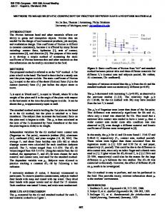
4.1 Effect of Displacement Rate. A series of friction measurements were conducted by sliding the upper specimen under various linear velocities. All tests were run under a constant normal load of 4.2 N and laboratory environmental conditions of 45% RH and 22.5° C. The total sliding distance was 1 mm, corresponding to several seconds of data, depending on the displacement rate. Because the focus of this paper is on the static friction measurement, these conditions were sufficient to capture the maximum friction force to initiate sliding. A typical measurement using the smooth interface I and a displacement rate of 200 ␮m / s is shown in Fig. 7. Time zero represents the start of the actuator motion. The friction force shown in Fig. 7共a兲 is zero before the application of any tangential force, it reaches a maximum value at 0.16 s 共corresponding to the static friction force兲, and then exhibits kinetic sliding friction, which may or may not be lower than the static friction value. The period from the start to t = 0.16 s corresponds to the microslip zone, where the friction force increases from zero to its maximum static friction value. This behavior is in general agreement with typical static-to-kinetic friction transitions, as reported elsewhere 关4,5兴. Figure 7共b兲 shows the in situ normal force and that it is approximately constant at 4.2 N, with small changes during the transition period. The small normal load change is associated with normal motions occurring during microslip transitions and referred to as “microjumps,” as reported in the literature, e.g., 关15兴. Figure 7共c兲 depicts the friction coefficient, which was obtained by dividing the friction force by the normal load. The converted encoder displacement from the encoder’s pulse signal is shown in Fig. 7共d兲. 758 / Vol. 129, OCTOBER 2007

repeatability

in

friction

coefficient

Note that only 0.5 s 共or 80 ␮m displacement兲 of data are shown in Fig. 7 because the remaining data 共to a total of 1 mm sliding distance兲 showed constant kinetic friction behavior. During the friction coefficient measurements, there were typically three experiments done for each condition. Figure 8 shows a typical repetition at a displacement rate of 200 ␮m / s. As can be seen, typical one standard deviation variation of the sliding friction was ⬍5%. Figure 9 shows representative static friction coefficient measurements versus time under different displacement rates, ranging from 50 ␮m / s to 500 ␮m / s, using smooth dry interface I. These experiments were repeatable as verified by multiple experiments under the same conditions. In all four cases shown, the static friction coefficient values can clearly be identified, with cases a and b 共slower velocities兲 showing a clear decrease from static to kinetic friction transition, while cases c and d 共faster velocities兲 do not exhibit a clear decrease from static to kinetic friction. Under slow sliding conditions, there will be more time to build up the static friction force 共due to, for example, asperity junction growth兲, which will result in a larger friction decrement from static to kinetic values. These results are in agreement with Ref. 关1兴. In all cases, the static friction coefficient values are relatively large, ⬃1, which is expected for smoother surfaces and could be attributed to strong adhesion at a smooth interface 关7,8兴. 4.2 Effect of Surface Conditions. The effect of surface conditions, such as roughness, the presence of wear debris, and

Fig. 9 Friction coefficient measurements under different sliding velocities, smooth interface I

Transactions of the ASME

Downloaded 19 Sep 2007 to 130.126.178.167. Redistribution subject to ASME license or copyright, see http://www.asme.org/terms/Terms_Use.cfm

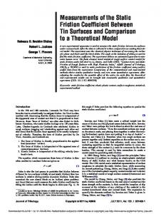
Fig. 10 Friction coefficient measurements under different surface conditions at 100 ␮m / s

minute traces of lubricant at the interface, on static friction coefficient was investigated next. Specifically, in practical applications, one finds wear particles and minute amounts of lubricant at the interface. The wear debris at the interface was generated by manually rubbing the samples against each other at a normal load of ⬃5 N in a reciprocating motion at a total of 200 times. This procedure generated ⬃15 ␮m size of wear particles as measured using a low magnification microscope. We do not believe that the generation of wear debris significantly affected the microhardness of the samples; however, it somewhat affected the surface topography. From visual observation of the affected areas, it was apparent that the largest topographical changes were scratches on the surfaces. Because the actual roughness was not quantified after these experiments, the static friction model was not used for this particular case and any future modeling of this interface will also need to include the actual surface roughness after the initial wear in period. In order to evaluate the presence of lubricant at the interface, the smooth interface I was used along with 2 mg of a commercially available polyolester lubricant added to the contact before testing to simulate boundary/mixed lubrication conditions. All tests were performed with a constant tangential displacement rate of 100 ␮m / s. Examining Fig. 10, the static friction coefficient values for the cases of boundary lubricant and wear debris presence for smooth interface I and for dry, rougher interface II are 0.30, 0.18, and 0.20, respectively. These values are significantly lower than the value of 1.18 for the dry smooth interface I case. Clearly, a smooth dry interface exhibits the highest static friction coefficient compared to a rougher, lubricated or wear debris-presence interface. Also, these results indicate that a method to reduce very high static friction values with smooth surfaces is to allow wear debris to be trapped at the interface and/or the presence of contaminants and/or minute traces of lubricants. Further testing was conducted to investigate the effect of dwell time for the case of boundary lubricated smooth interface I and low displacement rate of 50 ␮m / s. After 24 h of dwell, the static friction coefficient was increased from 0.27 to 0.37 as the trace of lubricant at the interface was squeezed out of the contact, in agreement with past research 关16兴. 4.3 Comparison With Simulation Results. As mentioned earlier, the KE rough surface friction model, which is valid for dry interfaces and does not capture any dynamic velocity effects, was used to predict the friction coefficient for the smooth and rough interfaces considered in this work. Shown in Fig. 11 are the simuJournal of Tribology

Fig. 11 Comparison of the static friction coefficient between theoretical „KE model… and experimental results under different sliding velocities

lation results for the cases of smooth interface I and ⌬␥ = 0.5 N / m and 0.01 N / m as well as rough interface II and ⌬␥ = 0.5 N / m, along with the experimental results. These results are plotted against displacement rate, which ranges from 50 ␮m / s to 500 ␮m / s. As expected, the modeled results are not able to capture the displacement rate effects and are shown as straight lines. The experimental results shown are the average values from multiple experiments for each different interfacial condition and a constant external load F = 4.2 N, where steady values of the static friction coefficient were predicted by the theoretical model. Examining the experimental results for the smooth dry interface I, the static friction coefficient values decrease with increasing displacement rate. On the other hand, in the presence of boundary lubrication 共interface I兲, the friction coefficient is almost independent of the displacement rate. This can be explained by the fact that even a trace of lubricant at the contact has a “smoothening” effect, not allowing individual asperities and small wear particles to substantially change the tangential contact characteristics, thus friction. The KE model should be able to predict the experimental results under dry conditions and in the absence of other complicating effects. To this extent, the modeled value for the interface I is 1.01, which matches very well with the experimental measurements at 200 ␮m / s. This is to be expected because, at lower velocities, asperity junction growth and creep effects may be taking place, whereas at faster velocities dynamic effects may play a more significant role. Similarly, for the rough case II, the model predicts a friction coefficient of 0.09 共extremely small value due to the large value of the plasticity index, ␺ = 2.79兲, whereas the measured value at 100 ␮m / s is higher at 0.2. This indicates that the KE model needs further improvement when plastic contacts are dominant, as shown in 关17兴 for a single asperity contact. In the above comparisons, the energy of adhesion used was ⌬␥ = 0.5 N / m for dry cases because the surfaces used were somewhat clean at ambient air conditions. Modeling friction in the presence of boundary lubrication is much more complicated that the case considered by KE because the lubricant also carries part of the normal load and the friction force arises from both shearing of the solid asperities as well as shearing of the lubricant 关18兴. In the absence of a basic rough static friction model to account for boundary lubrication, one may be tempted to use the simpler KE model because 共i兲 the amount of lubricant at the interface is miniscual and 共ii兲 the minute lubricant can be treated as a “contaminated” interface, thus reducing the adhesion energy, e.g., ⌬␥ OCTOBER 2007, Vol. 129 / 759

Downloaded 19 Sep 2007 to 130.126.178.167. Redistribution subject to ASME license or copyright, see http://www.asme.org/terms/Terms_Use.cfm

= 0.01 N / m. These conditions are also shown in Fig. 11, and the simulated friction coefficient is 0.72, which is much higher than the measured interface I boundary lubricated friction coefficient of 0.3. Clearly, the simpler KE model cannot capture the boundary lubrication phenomena by simply reducing the ⌬␥ value of the interface, and further improvements to the KE model, or a different model altogether, is needed to capture such phenomena. On the other hand, the KE model captures the roughness effects under dry conditions fairly well.

5

Conclusions

An apparatus was constructed and used to measure static friction under constant normal load and precise linear motion control. The in situ interfacial normal, friction, and lateral forces were precisely measured using a triaxial force transducer that was directly holding the stationary samples. Static friction measurements under different roughness and interface conditions were performed, ensuring repeatable results. The experimental results under dry conditions were favorably compared to an analytical elastic-plastic rough surface friction model. Specific findings from this study are as follows: 1. The smoother interface I exhibits higher static friction coefficient than the rougher interface II. The presence of wear debris and boundary lubrication significantly decreases the static friction coefficient compared to the dry interface. Also, a 24 h dwell time 共under boundary lubrication兲 increased the static friction coefficient as the trace of lubricant at the interface was squeezed out of the contact. 2. Under dry surface conditions, the static friction coefficient decreases with increasing displacement rate prior to sliding inception. However, for the boundary lubricated conditions, the static friction coefficient is almost independent of the displacement rate. 3. The KE elastic-plastic static friction model captures the experimental measurements well in terms of varying with changes in surface roughness under dry conditions. As expected, the KE model fails to capture the dynamic velocity effects, as well as the complications of adding wear debris and boundary lubricant at the interface. 4. In order to capture dynamic displacement rate effects, the presence of traces of lubricant and third body particles 共versus solid contact friction兲, further improvements in the existing static friction model or a different model altogether need to be developed.

Acknowledgment This research was supported in part by the National Science Foundation under CAREER Grant No. CMS-0239232.

Nomenclature An ⫽ nominal contact area b, c ⫽ constant coefficient for integrand in Eqs. 共2兲 and 共5兲 d ⫽ mean normal separation between rough surfaces, d* = d / ␴ E ⫽ composite elastic modulus for two contacting surfaces F ⫽ external normal force, F* = F / AnH Fs ⫽ adhesion force, Fs* = Fs / AnH

760 / Vol. 129, OCTOBER 2007

H h K P Q R Ra V ys z ␤ ⌬␥ ␧

␩ ␾ ␮ ␯ ␴ ⌿ ␻ ␻c

⫽ ⫽ ⫽ ⫽ ⫽ ⫽ ⫽ ⫽ ⫽ ⫽ ⫽ ⫽ ⫽ ⫽ ⫽ ⫽ ⫽ ⫽ ⫽ ⫽ ⫽

hardness of softer material separation based on surface heights material hardness factor, K = 0.454+ 0.41␯ normal contact load, P* = P / AnH static friction force, Q* = Q / AnH average radius of asperities centerline average incipient displacement rate of specimen h-d asperity height, z* = z / ␴ roughness parameter, ␩R␴ energy of adhesion equilibrium spacing, ␧* = ␧ / ␴ areal density of asperities distribution function of asperity heights static friction coefficient Poisson’s ratio standard deviation of asperity heights plasticity index, Eq. 共8兲 local interface, z-d critical interference at inception of plastic deformation, ␻*c = ␻c / ␴

References 关1兴 Gassenfeit, E. H., and Soom, A., 1988, “Friction Coefficient Measured at Lubricated Planar Contacts During Star-Up,” ASME J. Tribol., 110, pp. 533– 538. 关2兴 Polycarpou, A. A., and Etsion, I., 1998, “Comparison of the Static Friction Sub-Boundary Lubrication Model With Experimental Measurements on ThinFilm Disks,” Tribol. Trans., 41, pp. 217–224. 关3兴 Xie, W., De Meter, E. C., and Trethewey, M. W., 2000, “An Experimental Evaluation of Coefficients of Static Friction of Common Workpiece-Fixture Element Pairs,” Int. J. Mach. Tools Manuf., 40, pp. 467–488. 关4兴 Hwang, D. H., and Zum Gahr, K. H., 2003, “Transition from Static to Kinetic Friction of Unlubricated or Oil Lubricated Steel/Steel, Steel/Ceramic and Ceramic/Ceramic Pairs,” Wear, 255, pp. 365–375. 关5兴 Etsion, I., Levinson, O., Halperin, G., and Varenberg, M., 2005, “Experimental Investigation of the Elastic-Plastic Contact Area and Static Friction of Sphere on Flat,” ASME J. Tribol., 127, pp. 47–50. 关6兴 Greenwood, J. A., and Williamson, J. B. P., 1966, “Contact of Nominally Flat Surfaces,” Proc. R. Soc. London, Ser. A, 295, pp. 300–319. 关7兴 Chang, W. R., Etsion, I., and Bogy, D. B., 1987, “An Elastic-Plastic Model for the Contact of Rough Surfaces,” ASME J. Tribol., 109, pp. 257–263. 关8兴 Chang, W. R., Etsion, I., and Bogy, D. B., 1988, “Static Friction Coefficient Model for Metallic Rough Surfaces,” ASME J. Tribol., 110, pp. 57–63. 关9兴 Kogut, L., and Etsion, I., 2004, “A Static Friction Model for Elastic-Plastic Contacting Rough Surfaces,” ASME J. Tribol., 126, pp. 34–40. 关10兴 Jackson, R. L., and Green, I., 2005, “A Finite Element Study of Elasto-Plastic Hemispherical Contact Against a Rigid Flat,” ASME J. Tribol., 127共2兲, pp. 343–354. 关11兴 Yu, N., and Polycarpou, A. A., 2004, “Adhesive Contact Based on the Lennard-Jones Potential: A Correction to the Value of the Equilibrium Distance as Used in the Potential,” J. Colloid Interface Sci., 278共2兲, pp. 428–435. 关12兴 McCool, J. I., 1986, “Comparison of Models for the Contact of Rough Surfaces,” Wear, 107, pp. 37–60. 关13兴 Shi, X., and Polycarpou, A. A., 2005, “Measurement and Modeling of Normal Contact Stiffness and Contact Damping at the Meso Scale,” ASME J. Vibr. Acoust., 127, pp. 52–60. 关14兴 Rabinowitcz, E., 1995, Friction and Wear of Materials, 2nd ed., Wiley, New York. 关15兴 Sakamoto, T., 1987, “Normal Displacement and Dynamic Friction Characteristics in a Stick-Slip Process,” Tribol. Int., 20共11兲, pp. 25–31. 关16兴 Rabinowitcz, E., 1951, “The Nature of the Static and Kinetic Coefficient of Friction,” J. Appl. Phys., 22共11兲, pp. 1373–1379. 关17兴 Brizmer, V., Kligerman, Y., and Etsion, I., 2007, “Elastic–Plastic Spherical Contact Under Combined Normal and Tangential Loading in Full Stick,” Tribol. Lett., 25, pp. 61–70. 关18兴 Polycarpou, A. A., and Soom, A., 1996, “A Two-Component Mixed Friction Model for a Lubricated Line Contact,” ASME J. Tribol., 118, pp. 183–189.

Transactions of the ASME

Downloaded 19 Sep 2007 to 130.126.178.167. Redistribution subject to ASME license or copyright, see http://www.asme.org/terms/Terms_Use.cfm