[2] O. Beaumont, V. Boudet, A. Petitet, F. Rastello, and Y. Robert. A proposal ... [15] Paul Feautrier and Nadia Tawbi. Résolution de syst`emes d'inéquations ...
INSTITUT NATIONAL DE RECHERCHE EN INFORMATIQUE ET EN AUTOMATIQUE
Static load-balancing techniques for iterative computations on heterogeneous clusters H´el`ene Renard, Yves Robert, Fr´ed´eric Vivien
No 4745 February 2003
ISSN 0249-6399
ISRN INRIA/RR--4745--FR+ENG
` THEME 1
apport de recherche
Static load-balancing techniques for iterative computations on heterogeneous clusters H´el`ene Renard, Yves Robert, Fr´ed´eric Vivien Th`eme 1 — R´eseaux et syst`emes Projet ReMaP Rapport de recherche n˚4745 — February 2003 — 22Conclusionsection*.36 pages
Abstract: This paper is devoted to static load balancing techniques for mapping iterative algorithms onto heterogeneous clusters. The application data is partitioned over the processors. At each iteration, independent calculations are carried out in parallel, and some communications take place. The question is to determine how to slice the application data into chunks, and to assign these chunks to the processors, so that the total execution time is minimized. We establish a complexity result that assesses the difficulty of this problem, and we design practical heuristics that provide efficient distribution schemes. Key-words: Heterogeneous clusters, static load-balancing techniques, communication, complexity.
(R´ esum´ e : tsvp) This text is also available as a research report of the Laboratoire de l’Informatique du Parall´elisme http://www.ens-lyon.fr/LIP.
Unit´e de recherche INRIA Rhˆone-Alpes 655, avenue de l’Europe, 38330 MONTBONNOT ST MARTIN (France) T´el´ephone : 04 76 61 52 00 - International : +33 4 76 61 52 00 T´el´ecopie : 04 76 61 52 52 - International : +33 4 76 61 52 52
´ Equilibrage de charges pour algorithmes it´ eratifs sur plateformes h´ et´ erog` enes R´ esum´ e : Ce rapport est consacr´e `a l’´equilibrage de charge pour algorithmes it´eratifs sur plateformes h´er´erog`enes. Les donn´ees sont r´eparties sur l’ensemble des ` chaque it´eration, les calculs ind´ependants sont transmis en parall`ele ressources. A et les communications ont lieu. Le probl`eme est de d´eterminer comment partitionner les donn´ees et comment les r´epartir sur les ressources pour que le temps total d’ex´ecution soit minimal. Nous avons d´emontr´e un r´esultat de complexit´e qui ´etablit la difficult´e de ce probl`eme, et nous proposons des heuristiques pratiques qui prouvent l’efficacit´e de la distribution. Mots-cl´ e : plexit´e.
Grappes h´et´erog`enes, ´equilibrage de charge, communications, com-
Static load-balancing techniques on heterogeneous clusters
1
3
Introduction
In this paper, we investigate static load balancing techniques for iterative algorithms that operate on a large collection of application data. The application data will be partitioned over the processors. At each iteration, some independent calculations will be carried out in parallel, and then some communications will take place. This scheme is very general, and encompasses a broad spectrum of scientific computations, from mesh based solvers (e.g. elliptic PDE solvers) to signal processing (e.g. recursive convolution), and image processing algorithms (e.g. mask-based algorithms such as thinning). The target architecture is a fully heterogeneous cluster, composed of differentspeed processors that communicate through links of different capacities. The question is to determine the best partitioning of the application data. The difficulty comes from the fact that both the computation and communication capabilities of each resource must be taken into account. An abstract view of the problem is the following: the iterative algorithm repeatedly operates on a large rectangular matrix of data samples. This data matrix is split into vertical slices that are allocated to the computing resources (processors). At each step of the algorithm, the slices are updated locally, and then boundary information is exchanged between consecutive slices. This (virtual) geometrical constraint advocates that processors be organized as a virtual ring. Then each processor will only communicate twice, once with its (virtual) predecessor in the ring, and once with its successor. There is no reason a priori to restrict to a uni-dimensional partitioning of the data, and to map it onto a uni-dimensional ring of processors: more general data partitionings, such as two-dimensional, recursive, or even arbitrary slicings into rectangles, could be dealt with. But uni-dimensional partitionings are very natural for most applications, and, as will be shown in this paper, the problem to find the optimal one is already very difficult. We assume that the target computing platform can be modeled as a complete graph: • Each vertex in the graph models a computing resource Pi , and is weighted by the relative cycle-time of the resource. Of course the absolute value of the time-unit is application-dependent, what matters is the relative speed of one processor versus the other. • Each edge models a communication link, and is weighted by the relative capacity of the link. Assuming a complete graph means that there is a virtual communication link between any processor pair Pi and Pj . Note that this link
RR n˚4745
4
H. Renard, Y. Robert, F. Vivien
does not necessarily need to be a direct physical link. There may be a path of physical communication links from Pi to Pj : if the slowest link in the path has maximum capacity ci,j , then the weight of the edge will be ci,j . We suppose that the communication capacity ci,j is granted between Pi and Pj (so if some communication links happen to be physically shared, we assume that a fraction of the total capacity, corresponding to the inverse of ci,j , is available for messages from Pi to Pj ). This assumption of a fixed capacity link between any processor pair makes good sense for interconnection networks based upon high-speed switches like Myrinet [12]. Given these hypotheses, the optimization problem that we want to solve is the following: how to slice the matrix data into chunks, and assign these chunks to the processors, so that the total execution time for a given sweep step, namely a computation followed by two neighbor communications, is minimized? We have to perform resource selection, because there is no reason a priori that all available processors will be involved in the optimal solution (for example some fast computing processor may be left idle because its communication links with the other processors are too slow). Once some resources have been selected, they must be arranged along the best possible ring, which looks like a difficult combinatorial problem. Finally, once a ring has been set up, there remains to load-balance the workloads of the participating resources The rest of the paper is organized as follows. In Section 2, we formally state the previous optimization problem, which we denote as SliceRing. If the network is homogeneous (all links have same capacity), then SliceRing can be solved easily, as shown in Section 3. But in the general case, SliceRing turns out to be a difficult problem: we show in Section 4 that the decision problem associated to SliceRing is NP-complete, as could be expected from its combinatorial nature. After the proof of this result, we derive in Section 5 a formulation of the SliceRing problem in terms of an integer linear program, thereby providing a (costly) way to determine the optimal solution. In Section 6, we move to the design of polynomial-time heuristics, and we report some experimental data. We survey related work in Section 7, and we provide a brief comparison of static versus dynamic strategies. Finally, we state some concluding remarks in Section 8.
2
Framework
In this section, we formally state the optimization problem to be solved. As already said, the target computing platform is modeled as a complete graph G = (P, E).
INRIA
Static load-balancing techniques on heterogeneous clusters
5
Each node Pi in the graph, 1 ≤ i ≤ |P | = p, models a computing resource, and is weighted by its relative cycle-time wi : Pi requires S.wi time-units to process a task of size S. Edges are labeled with communication costs: the time needed to transfer a message of size L from Pi to Pj is L.ci,j , where ci,j is the capacity of the link, i.e. the inverse of its bandwidth. The motivation to use a simple linear-cost model, rather than an affine-cost model involving start-ups, both for the communications and the computations, is the following: only large-scale applications are likely to be deployed on heterogeneous platforms. Each step of the algorithm will be both computation- and communication-intensive, so that start-up overheads can indeed be neglected. Anyway, most of the results presented here extend to an affine cost modeling, τi + S.wi for computations and βi,j + L.ci,j for communications. Let W be the total size of the work to be performed at each step of the algorithm. Processor Pi will P accomplish a share αi .W of this total work, where αi ≥ 0 for 1 ≤ i ≤ p and pi=1 αi = 1. Note that we allow αj = 0 for some index j, meaning that processor Pj do not participate in the computation. Indeed, there is no reason a priori for all resources to be involved, especially when the total work is not so large: the extra communications incurred by adding more processors may slow down the whole process, despite the increased cumulated speed. We will arrange the participating processors along a ring (yet to be determined). After updating its data slice, each active processor Pi sends some boundary data to its neighbors: let pred(i) and succ(i) denote the predecessor and the successor of Pi in the virtual ring. Then Pi requires H.ci,succ(i) time-units to send a message of size H to its successor, plus H.ci,pred(i) to receive a message of same size from its predecessor. In most situations, we will have symmetric costs (ci,j = cj,i ) but we do not make this assumption here. To illustrate the relationship between W and H, we can view the original data matrix as a rectangle composed of W columns of height H, so that one single column is exchanged between any pair of consecutive processors in the ring (but clearly, the parameter H can represent any fixed volume of communication). The total cost of a single step in the sweep algorithm is the maximum, over all participating processors, of the time spent computing and communicating: Tstep = max I{i}[αi .W.wi + H.(ci,succ(i) + ci,pred(i) )] 1≤i≤p
where I{i}[x] = x if Pi is involved in the computation, and 0 otherwise. In summary, the goal is to determine the best way to select q processors out of the p available, and to arrange them along a ring so that the total execution time per step is minimized. We formally state this optimization problem as follows:
RR n˚4745
6
H. Renard, Y. Robert, F. Vivien
Definition 1 (SliceRing(p,wi ,ci,j ,W ,H)). Given p processors of cycle-times wi and p(p − 1) communication links of capacity ci,j , given the total workload W and the communication volume H at each step, determine � Tstep = min min max ασ(i) .W.wσ(i) + H.(cσ(i),σ(i−1 mod q) + cσ(i),σ(i+1 mod q) ) 1≤q≤p 1≤i≤q σ ∈ S q,p Pq α = 1 i=1 σ(i) (1) Here Sq,p denotes the set of one-to-one functions σ : [1..q] → [1..p] which index the q selected processors, for all candidate values of q between 1 and p. From Equation 1, we see that the optimal solution will involve all processors as soon as the ratio W H is large enough: in that case, the impact of the communications becomes smaller in front of the cost of the computations, and these computations should be distributed to all resources. But even in that case, we still have to decide how to arrange the processors along a ring. Extracting the “best” ring out of the interconnection graph seems to be a difficult combinatorial problem. Before assessing this result (see Section 4), we deal with the much easier situation when the network is homogeneous (see Section 3). To conclude this section, we point out that this framework is more general than iterative algorithms: in fact, our approach applies to any problem where independent computations are distributed over heterogeneous resources. The only hypothesis is that the communication volume is the same between adjacent processors, regardless of their relative workload.
3
Homogeneous networks
Solving the optimization problem, i.e. minimizing expression (1), is easy when all communication times are equal. This corresponds to a homogeneous network where each processor pair can communicate at the same speed, for instance through a bus or an Ethernet backbone. Let us assume that ci,j = c for all i and j, where c is a constant. There are only two cases to consider: (i) only the fastest processor is active; (ii) all processors are involved. Indeed, as soon as a single communication occurs, we can have several ones for the same cost, and the best is to divide the computing load among all resources. In the former case (i), we derive that Tstep = W.wmin , where wmin is the smallest cycle-time. In the latter case (ii), the load is most balanced when the execution time
INRIA
Static load-balancing techniques on heterogeneous clusters
7
is the same for all processors: otherwise, removing a small portion of the load of the processor with largest execution time, and giving it to a processor finishing earlier, would decrease P the maximum computation time. This leads to αi .wi = Constant for all i, with pi=1 αi = 1. We derive that Tstep = W.wcumul + 2H.c, where wcumul = Pp 1 1 . i=1 wi
We summarize these results as follows:
Proposition 1. The optimal solution to SliceRing(p,wi ,c,W ,H) is Tstep = min {W.wmin , W.wcumul + 2H.c} where wmin = min1≤i≤p wi and wcumul =
Pp 1
1 i=1 wi
.
If the platform is given, there is a threshold, which is application-dependent, to decide whether only the fastest computing resource, as opposed to all the resources, should be involved. Given H, the fastest processor will do all the job for small values 2c of W , namely W ≤ H. wmin −w . Otherwise, for larger values of W , all processors cumul should be involved.
4
Complexity
The decision problem associated to the SliceRing optimization problem is the following: Definition 2 (SliceRingDec(p,wi ,ci,j ,W ,H,K)). Given p processors of cycletimes wi and p(p − 1) communication links of capacity ci,j , given the total workload W and the communication volume H at each step, and given a time bound K, is it possible to find an integer q ≤ p, aP one-to one mapping σ : [1..q] → [1..p], and nonnegative rational numbers αi with qi=1 ασ(i) = 1, such that � Tstep = max ασ(i) .W.wσ(i) + H.(cσ(i),σ(i−1 mod q) + cσ(i),σ(i+1 mod q) ) ≤ K? 1≤i≤q
The following result states the intrinsic difficulty of the problem: Theorem 1. SliceRingDec(p,wi ,ci,j ,W ,H,K) is NP-complete. Proof. Obviously, SliceRingDec belongs to NP. To prove its completeness, we use a reduction from HamCycle, the Hamiltonian Cycle Problem, which is NPcomplete [17]. Consider an arbitrary instance I1 of HamCycle: given a graph
RR n˚4745
8
H. Renard, Y. Robert, F. Vivien
Gh = (Vh , Eh ), is there a Hamiltonian cycle in Gh , i.e. a cycle that visits all the vertices of G exactly once? We construct the following instance I2 of SliceRingDec: we let p = |Vh | (assume p ≥ 2 without loss of generality), and we define a complete interconnection graph G = (P, E), whose edge costs are given by � ce =
ε if e ∈ Eh 2 otherwise
where 0 < ε < 12 is a small constant. We let W = H = 1 and wi = p for 1 ≤ i ≤ p. Clearly, I2 can be constructed in time polynomial in the size of I1 . Finally, we let K = 1 + 2ε. Assume first that I1 has a solution, i.e. that Gh possesses a hamiltonian cycle. We use the edges of this path to build the ring. All processors are involved, and we let αi = 1/p for 1 ≤ i ≤ p. The execution time and the communication time are the same for all processors, we obtain that Tstep = 1p · p + 2ε = K, hence a solution to I2 . Assume now that I2 has a solution. If a single processor were participating in that solution, then we would have Tstep = 1.p ≥ 2 > K, a contradiction. Hence there are q processors, with q ≥ 2, participating in the solution. If the ring used a communication edge that did not belong to Gh , then the cost of that edge would be 2 and Tstep ≥ H.2 = 2 > K, again a contradiction. There remains to show that we do use all the p processors in the solution. But otherwise, if q < p, one computation load would be at least equal to 1q .W.p > 1, which would imply that Tstep > K. Finally, q = p, and the edges of the solution ring define a Hamiltonian cycle in Gh , thereby providing a solution to I1 .
5
ILP formulation
When the network is heterogeneous, we face a complex situation: how to determine the number of processors that should take part to the computation already is a difficult question. In this section, we express the solution to the SliceRing optimization problem, in terms of an Integer Linear Programming (ILP) problem. Of course the complexity of this approach may be exponential in the worst case, but it will provide useful hints to design low-cost heuristics. We start with the case where all processors are involved in the optimal solution. We extend the approach to the general case later on.
INRIA
Static load-balancing techniques on heterogeneous clusters
9
time
α1 .W.w1
α2 .W.w2 α3 .W.w3 H.c2,3
H.c1,2 H.c1,5
H.c2,1
p1
p2
α4 .W.w4
H.c3,4 H.c3,2
H.c4,5 H.c4,3
p3
α5 .W.w5
H.c5,1 H.c5,4
p4
p5
processors
Figure 1: Summary of computation and communication times with p processors.
5.1
When all processors are involved
Assume first that all processors are involved in an optimal solution. All the p processors require the same amount of time to compute and communicate: otherwise, we would slightly decrease the computing load of the last processor to complete its assignment (computations followed by communications) and assign extra work to another one. Hence (see Figure 1 for an illustration) we have Tstep = αi .W.wi + H.(ci,i−1 + ci,i+1 )
(2)
for all i (indices in the communication costs are taken modulo p). Since P T −H.(ci,i−1 +ci,i+1 ) we derive that pi=1 step = 1. Defining wcumul = P p 1 W.wi we have:
Pp
1 i=1 wi
p Tstep H X ci,i−1 + ci,i+1 =1+ W.wcumul W wi
i=1 αi
= 1, as before,
(3)
i=1
P c +c Therefore, Tstep will be minimal when pi=1 i,i−1wi i,i+1 is minimal. This will be achieved for the ring that corresponds to the shortest hamiltonian cycle in the graph c +c G = (P, E), where each edge ei,j is given the weight di,j = i,jwi j,i . Once we have this path, we derive Tstep from Equation 3, and then we determine the load αi of each processor using Equation 2. To summarize, we have the following result:
RR n˚4745
10
H. Renard, Y. Robert, F. Vivien
Proposition 2. When all processors are involved, finding the optimal solution is equivalent to solving the Traveling Salesman Problem in the weighted graph (P, E, d), c +c di,j = i,jwi j,i . Of course we are not expecting any polynomial-time solution from this result, because the decision problem associated to the Traveling Salesman Problem is NPcomplete [17] (even worse, because the distance d does not satisfy the triangle inequality, there is no polynomial-time approximation [9]), but this equivalence gives us two lines of action: • For platforms of reasonable size, the optimal solution can be computed using an integer linear program that returns the optimal solution to the Traveling Salesman Problem • For very large platforms, we can use well-established heuristics which approximate the solution to the Traveling Salesman Problem in polynomial time, such as the Lin-Kernighan heuristic [23, 18]. In the following , we briefly recall the classical formulation of the Traveling Salesman Problem as an Integer Linear Programming (ILP) problem. This will solve our problem whenever all processors are involved. In Section 5.2 we will extend the ILP formulation to cope with the case where only a fraction of the computing resources are involved in the optimal solution. Consider the complete weighted graph G = (P, E, d), where |P | = p, and assume that we start the tour, i.e. the processor ring, with processor P1 . Let xi,j be integer variables such that xi,j = 1 when Pj is the processor immediately following Pi in the tour, andPxi,j = 0 otherwise. Since exactly one processor Pp precedes Pj in the tour, we have pi=1 xi,j = 1 for each j. Similarly, we have j=1 xi,j = 1 for each i. The P P cost of the tour can be expressed as pi=1 pj=1 di,j .xi,j . But these equations are not sufficient: we have to exclude the case of two or more disjoint sub-tours. To this purpose, we introduce p − 1 new integer variables u2 , u3 , . . . , up with ui ≥ 0 and (p − 1)(p − 2) new constraints as follows: ui − uj + p.xi,j ≤ p − 1 for 2 ≤ i, j ≤ p, i 6= j Intuitively, ui represents the position on the tour at which Pi is visited, and the constraints ensures that the tour does not split into sub-tours. Indeed, we follow the proof in [11]. Suppose first that we have a Hamiltonian cycle (“starting” in P1 ): we prove that the ILP problem has a solution. Let ui be the position on the path at which Pi is visited (excluding P1 , and counting from 0). For instance with p = 5 and
INRIA
Static load-balancing techniques on heterogeneous clusters
11
the tour P1 → P4 → P2 → P3 → P5 → P1 , then u4 = 0, u2 = 1, u3 = 2, and u5 = 3. We have 0 ≤ ui ≤ p − 2 for i ≥ 2. Therefore if xi,j = 0, ui − uj + p.xi,j ≤ p − 2 if i 6= j, and the inequality holds. Next, if xi,j = 1, Pj is visited immediately after Pi , hence uj = ui + 1, and ui − uj + p.xi,j = p − 1, and the inequality holds again. Conversely, suppose that we have a solution to the ILP problem, and assume that the tour splits into at least two sub-tours. Then, there is a sub-tour of r ≤ p − 1 processors that does not include P1 . Adding up the r equations for the r non-zero values of xi,j of that sub-tour leads to r.p ≤ r.(p − 1) (all the ui occur twice and cancel), a contradiction. Finally, we are led to the following ILP formulation:
TSP integer Pp linear Pp programming formulation Minimize i=1 j=1 di,j .xi,j , subject Ppto (1) xi,j = 1 1≤i≤p Pj=1 p 1≤j≤p (2) i=1 xi,j = 1 (3) xi,j ∈ {0, 1} 1 ≤ i, j ≤ p (4) ui − uj + p.xi,j ≤ p − 1 2 ≤ i, j ≤ p, i 6= j (5) ui integer, ui ≥ 0 2≤i≤p
Proposition 3. When all processors are involved, finding the optimal solution is equivalent to solving the previous integer linear program.
5.2
General case
How to extend the ILP formulation to the general case? For each possible value of q, 1 ≤ q ≤ p, we will set up an ILP problem giving the optimal solution with exactly q participating resources. Taking the smallest solution among the p values returned by these ILP problems will lead to the optimal solution. For a fixed value of q, 1 ≤ q ≤ p, we use a technique similar to that of Section 5.1, but we need additional variables. Here is the ILP:
RR n˚4745
12
H. Renard, Y. Robert, F. Vivien
q-ring integer programming formulation Pp linear Pp Minimize d i=1 j=1 i,j .xi,j , subject to P P (1) Ppi=1 xi,j = pi=1 xj,i 1≤j≤p p (2) x ≤ 1 1 ≤j≤p i,j Pi=1 p Pp (3) i=1 j=1 xi,j = q (4) xP ∈ {0, 1} 1 ≤ i, j ≤ p i,j p (5) i=1 yi = 1 (6) − p.yi − p.yj + ui − uj + q.xi,j ≤ q − 1 1 ≤ i, j ≤ p, i 6= j (7) y ∈ {0, 1} 1≤i≤p i (8) ui integer, ui ≥ 0 1≤i≤p As before, the intuitive idea is that xi,j = 1 if and only if Pj is the immediate successor of Pi in the q-ring. Constraints (1) and (2) state that the in-degree of each node is the same as its out-degree, and will be equal to 0 or 1. Constraint (3) ensures that the ring is indeed composed of q processors. From constraints (5) and (7), we see that a single yi will be non-zero, and it represents the “origin” of the q-ring. Assume the non-zero value is y1 . For i = 1 and any value of j, constraint (6) will be satisfied because of the term −p.y1 . If neither i nor j is equal to the origin P1 , then constraint (6) reduces to constraint (4) of the TSP program, and assesses that the q-ring is not split into sub-rings. In the solution, ui = 0 for the origin and the non-participating nodes, and ui is the position after the origin (numbered from 0 to q − 2) of node Pi in the ring. We summarize these results as follows: Proposition 4. The SliceRing optimization problem can be solved by computing the solution of p integer linear programs, where p is the total number of resources.
6
Heuristics and experiments
After the previous theoretically-oriented results, we adopt a more practical approach in this section. We aim at deriving polynomial-time heuristics for solving the SliceRing optimization problem. Having expressed the problem in terms of a collection of integer linear programs enables us to compute the optimal solution with softwares like PIP [15, 14] or LP SOLVE [4] (at least for reasonable sizes of the target computing platforms). We
INRIA
Static load-balancing techniques on heterogeneous clusters
13
compare this optimal solution with that returned by two polynomial-time heuristics, one that approximates the TSP problem (but only returns a solution where all processors are involved), and a greedy heuristic that iteratively grows the solution ring.
6.1
TSP-based heuristic
The situation where all processors are involved in the optimal solution is very important in practice. Indeed, only very large applications are likely to be deployed on distributed heterogeneous platforms. And when W is large enough, we know from Equation 1 that all processors will be involved. From Section 5.1 we know that the optimal solution, when all processors are involved, corresponds to the shortest Hamiltonian cycle in the graph (P, E, d), with c +c di,j = i,jwi j,i . We use the well-known Lin-Kernighan heuristic [23, 18], to approximate this shortest path. By construction, the TSP-based heuristic always returns a solution where all processors are involved. Of course, if the optimal solution requires fewer processors, the TSP-based heuristic will fail to find it.
6.2
Greedy heuristic
The greedy heuristic starts by selecting the fastest processor. Then, it iteratively includes a new node in the current solution ring. Assume that we have already selected a ring of r processors. For each remaining processor Pi , we search where to insert it in the current ring: for each pair of successive processors (Pj , Pk ) in the ring, we compute the cost of inserting Pi between Pj and Pk in the ring. We retain the processor and the pair that minimize the insertion cost, and we store the value of Tstep . This step of the heuristic has a complexity proportional to (p − r).r. Finally, we grow the ring until we have p processors. and we return the minimal Pp value obtained for Tstep . The total complexity is r=1 (p − r)r = O(p3 ). Note that it is important to try all values of r, because Tstep may not vary monotically with r.
6.3
Platform description
We experimented with two platforms, one located in ENS Lyon and the other in the University of Strasbourg. Figure 2 represents the Lyon platform, which is composed of 14 processors, whose cycle-times are described in Table 1. Table 2 shows the capacity of the links, i.e. the inverse of the bandwidth, between each processor pair (Pi , Pj ).
RR n˚4745
14
H. Renard, Y. Robert, F. Vivien
moby
router backbone routlhpc
canaria
sci2 sci1 myri1
sci3 mryi0
Hub
popc0
sci0
Switch sci4
myri2 sci6
sci5
Hub
Figure 2: Topology of the Lyon platform.
P0 0.0291
P1 0.00874
P2 0.0206
P3 0.0451
P4 0.0206
P5 0.0291
P6 0.0206
P7 0.0206
P8 0.0206
P9 0.0206
P10 0.0206
P11 0.0206
P12 0.0206
P13 0.0206
Table 1: Processor cycle-times (in seconds per megaflop) for the Lyon platform. P0 P0 P1 P2 P3 P4 P5 P6 P7 P8 P9 P10 P11 P12 P13
0.198 1.702 1.702 0.262 0.198 1.702 1.702 0.262 0.262 0.262 0.262 0.262 0.262
P1 0.198 1.702 1.702 0.262 0.198 1.702 1.702 0.262 0.262 0.262 0.262 0.262 0.262
P2 1.702 1.702 0.248 0.248 1.702 0.248 0.248 0.248 0.248 0.248 0.248 0.248 0.248
P3 1.702 1.702 0.248 0.248 1.702 0.248 0.248 0.248 0.248 0.248 0.248 0.248 0.248
P4 0.262 0.262 0.248 0.248 0.262 0.248 0.248 0.248 0.248 0.248 0.248 0.248 0.248
P5 0.198 0.198 1.702 1.702 0.262 1.702 1.702 0.262 0.262 0.262 0.262 0.262 0.262
P6 1.702 1.702 0.248 0.248 0.248 1.702 0.248 0.248 0.248 0.248 0.248 0.248 0.248
P7 1.702 1.702 0.248 0.248 0.248 1.702 0.248 0.248 0.248 0.248 0.248 0.248 0.248
P8 0.262 0.262 0.248 0.248 0.248 0.262 0.248 0.248 0.248 0.248 0.248 0.248 0.248
P9 0.262 0.262 0.248 0.248 0.248 0.262 0.248 0.248 0.248 0.248 0.248 0.248 0.248
P10 0.262 0.262 0.248 0.248 0.248 0.262 0.248 0.248 0.248 0.248 0.248 0.248 0.248
P11 0.262 0.262 0.248 0.248 0.248 0.262 0.248 0.248 0.248 0.248 0.248 0.248 0.248
P12 0.262 0.262 0.248 0.248 0.248 0.262 0.248 0.248 0.248 0.248 0.248 0.248
P13 0.262 0.262 0.248 0.248 0.248 0.262 0.248 0.248 0.248 0.248 0.248 0.248 0.248
0.248
Table 2: Capacity of the links (time in seconds to transfer a one-megabit message) for the Lyon platform.
Similarly, Figure 3 represents the Strasbourg platform, which is composed of 13 processors, whose cycle-times are described in Table 3, while Table 4 shows the capacity of the links.
INRIA
Static load-balancing techniques on heterogeneous clusters
15
gauvain guenievre
dinadan caseb
pellinore Switch nestea
router
router
sekhmet darjeeling
marathon
lattice
lancelot
shaitan
merlin
Figure 3: Topology of the Strasbourg platform.
P0 0.00874
P1 0.00874
P2 0.0102
P3 0.00728
P4 0.00728
P5 0.0262
P6 0.00583
P7 0.016
P8 0.00728
P9 0.00874
P10 0.0131
P11 0.00583
P12 0.0131
Table 3: Processor cycle-times (in seconds per megaflop) for the Strasbourg platform. P0 P0 P1 P2 P3 P4 P5 P6 P7 P8 P9 P10 P11 P12
0.048 0.019 0.017 0.019 0.147 0.151 0.154 0.147 0.048 0.017 0.016 0.151
P1 0.048 0.048 0.048 0.048 0.147 0.151 0.154 0.147 0.017 0.048 0.048 0.151
P2 0.019 0.048 0.019 0.019 0.147 0.151 0.154 0.147 0.048 0.019 0.019 0.151
P3 0.017 0.048 0.019 0.019 0.147 0.151 0.154 0.147 0.048 0.017 0.018 0.151
P4 0.019 0.048 0.019 0.019 0.147 0.151 0.154 0.147 0.048 0.019 0.019 0.151
P5 0.147 0.147 0.147 0.147 0.147 0.151 0.154 0.147 0.147 0.147 0.147 0.151
P6 0.151 0.151 0.151 0.151 0.151 0.151 0.154 0.151 0.151 0.151 0.151 0.151
P7 0.154 0.154 0.154 0.154 0.154 0.154 0.154 0.154 0.154 0.154 0.154 0.154
P8 0.147 0.147 0.147 0.147 0.147 0.147 0.151 0.154 0.147 0.147 0.147 0.151
P9 0.048 0.017 0.048 0.048 0.048 0.147 0.151 0.154 0.147 0.048 0.048 0.151
P10 0.017 0.048 0.019 0.017 0.019 0.147 0.151 0.154 0.147 0.048 0.018 0.151
P11 0.016 0.048 0.019 0.018 0.019 0.147 0.151 0.154 0.147 0.048 0.018
P12 0.151 0.151 0.151 0.151 0.151 0.151 0.151 0.154 0.151 0.151 0.151 0.151
0.151
Table 4: Capacity of the links (time in seconds to transfer a one-megabit message) for the Strasbourg platform.
6.4
Results
For both topologies, we compared the greedy heuristic against the optimal solution obtained with integer linear programming softwares, when available. Since LP SOLVE fails to compute the result when more than five processors are involved, we only report the results of the PIP software. Tables 5 and 6 show the difference
RR n˚4745
16
H. Renard, Y. Robert, F. Vivien
between the greedy heuristic and the optimal solution (computed with PIP) on the Lyon and Strasbourg platforms. The numbers in the tables represent the minimal cost of a path of length q on the platform, i.e. the value of the objective function of the ILP program of Section 5.2 (multiplied by a scaling factor 6000, because PIP needs a matrix of integers). PIP is able to compute the optimal solution for all values for the Strasbourg platform, but fails to do so between 9 and 13 processors for the Lyon platform (note that we used a machine with two gigabytes of RAM!). When all processors are involved, we also tried the LKH heuristic: for both platforms, it returns the optimal result. The conclusions that can be drawn from these experiments are the following: • the greedy heuristic is both fast and efficient, within 11.2% of the optimal for the Lyon platform, and 6.8% for the Strasbourg platform • the LKH heuristic is very reliable, but its application is limited to the case where all resources are involved • integer linear programming softwares rapidly fail to compute the optimal solution ``` ``` ``Processors ``` Heuristics ```
Greedy PIP
3
4
5
6
7
8
9
10
11
12
13
14
1202
556
1152
906
2240
3238
556
1128
906
2075
3071
5234 out of memory
6232 out of memory
7230 out of memory
8228 out of memory
10077
878
4236 out of memory
9059
Table 5: Comparison between the greedy heuristic and PIP for the Lyon platform. ``` ``` Processors ``` ``` Heuristics ``
3
4
5
6
7
8
9
10
11
12
13
Greedy PIP
1520 1517
2112 2109
3144 3141
3736 3733
4958 4955
5668 5660
7353 7348
8505 8500
10195 10188
12490 12235
15759 14757
Table 6: Comparaison between the greedy heuristic and PIP for the Strasbourg platform. In Figures 4 and 5, we plot the number popt of processors in the optimal solution as a function of the ratio W/H. As expected, when this ratio grows (meaning more computations per communication), more and more processors are used in the optimal solution, and the value of popt increases. Because the interconnection network of the Lyon platform involves links of similar capacities, the value of popt jumps from 1
INRIA
Static load-balancing techniques on heterogeneous clusters
17
(sequential solution) to 14 (all processors participate), while the greedy heuristic returns a solution with 6 processors in between. The big jump from 1 to 14 is easily explained: once there is enough work to make a communication affordable, rather use many communications for the same price, thereby better sharing the load. The interconnection network of the Strasbourg platform is more heterogeneous, and there the value of popt jumps from 1 (sequential solution) to 10, 11 and 13 (all processors participate), while the greedy heuristic closely follows this evolution. Comparaison between exact solution and greedy heuristic on the Lyon platform
Number of processors in the best solution
14
12
10
8
6
4
2 Exact solution Greedy heurisctic 0 0
5
10
15
20 W/H
25
30
35
40
Figure 4: Optimal number of processors for the Lyon platform.
7
Related work
Load balancing strategies have been widely studied, both for homogeneous platforms (see the collection of papers [26]) and for heterogeneous clusters (see chapter 25 in [6]). Distributing the computations (together with the associated data) can be performed either dynamically or statically, or a mixture of both. The vast majority of the literature deals with dynamic strategies, that calls for periodic re-mapping phases to remedy observed load-imbalance. Even though we target static schemes, we briefly discuss a few important references in the field of dynamic approaches. Simple paradigms are based upon the idea “use the past to predict the future”, i.e. use the currently observed speed of computation of each machine to decide for the next distribution of work [7, 8, 5]. Several authors [25, 24,
RR n˚4745
18
H. Renard, Y. Robert, F. Vivien
Comparaison between exact solution and greedy heuristic on the Strasbourg platform
Number of processors in the best solution
14
12
10
8
6
4
2 Exact solution Greedy heuristic 0 0
5
10
15
20 W/H
25
30
35
40
Figure 5: Optimal number of processors for the Strasbourg platform.
27, 19] propose a mapping policy which dynamically minimizes system degradation (including the cost of remapping) for each computation step. Other papers [28, 13] advocate local schemes where data is exchanged only between neighbor processors. Generally speaking, there is a challenge in determining a trade-off between the data distribution parameters and the process spawning and possible migration policies. Redundant computations might also be necessary to use a heterogeneous platform at its best capabilities. In the context of a library oriented approach, dynamic strategies are difficult to introduce, because they imply a complicated memory management. Static strategies are less general but prove useful if enough knowledge can be injected in the scheduling and mapping decision process. In other words, if the characteristics of the target platform (processor speeds and link capacities) and of the target application (computation and communication costs associated to each data chunk) are known rather accurately, then excellent performance can be achieved through static strategies. However, sophisticated data distribution schemes (like the ones presented in this paper) are mandatory to achieve such a good performance. Several authors have dealt with the static implementation of linear algebra kernels on heterogeneous platforms. Matrix multiplication has been studied by [22, 2]. LU and QR decomposition have been discussed by Barbosa et al. [1]. Static partitioning schemes to map a two-dimensional data matrix onto heterogeneous resources have been investigated by Crandall and Quinn [10], Kaddoura, Ranka and Wang [21],
INRIA
Static load-balancing techniques on heterogeneous clusters
19
and Beaumont et al. [3]. The main conclusions of these papers are drawn for three kinds of problems: • Distributing independent chunks of work to uni-dimensional (linear) arrays of heterogeneous processors is easy (see the algorithm in [2]) • Distributing independent chunks of work to two-dimensional processor grids is difficult. We have to search for the best distribution of work for each processor arrangement along the two-dimensional grid, and there is an exponential number of such arrangements as the grid size increases (see [1, 2]) • Relaxing the geometrical constraints induced by two-dimensional grids leads to irregular partitionings [10, 21, 3] that allow for a good load-balancing but are much more difficult to implement In this perspective, this paper shows that the first problem, i.e. distributing independent chunks of work to uni-dimensional processor arrays, is no longer easy when communications are taken into account in addition to computations. Finally, a survey of static load balancing techniques for mesh computations has been written by Hu and Blake [19]. On the same subject, see also the paper by Ichikawa and Yamashita [20].
8
Conclusion
The major limitation to programming heterogeneous platforms arises from the additional difficulty of balancing the load. Data and computations are not evenly distributed to processors. Minimizing communication overhead becomes a challenging task. Load balancing techniques can be introduced dynamically or statically, or a mixture of both. On one hand, we may think that dynamic strategies are likely to perform better, because the machine loads will be self-regulated, hence self-balanced, if processors pick up new tasks just as they terminate their current computation. However, data dependences, in addition to communication costs and control overhead, may well lead to slow the whole process down to the pace of the slowest processors. On the other hand, static strategies will suppress (or at least minimize) data redistributions and control overhead during execution. Furthermore, in the context of a scientific library, static allocations seem to be necessary for a simple and efficient
RR n˚4745
20
H. Renard, Y. Robert, F. Vivien
memory allocation. We agree, however, that targeting larger platforms such as distributed collections of heterogeneous clusters, e.g. available from the metacomputing grid [16], may well enforce the use of dynamic schemes. One major result of this paper is the NP-completeness of the SliceRing problem. Rather than the proof, the result itself is interesting, because it provides yet another evidence of the intrinsic difficulty of designing heterogeneous algorithms. But this negative result should not be over-emphasized. Indeed, another important contribution of this paper is the design of efficient heuristics, that provide a pragmatic guidance to the designer of iterative scientific computations. Implementing such computations on commodity clusters made up of several heterogeneous resources is a promising alternative to using costly supercomputers.
References [1] J. Barbosa, J. Tavares, and A. J. Padilha. Linear algebra algorithms in a heterogeneous cluster of personal computers. In 9th Heterogeneous Computing Workshop (HCW’2000), pages 147–159. IEEE Computer Society Press, 2000. [2] O. Beaumont, V. Boudet, A. Petitet, F. Rastello, and Y. Robert. A proposal for a heterogeneous cluster ScaLAPACK (dense linear solvers). IEEE Trans. Computers, 50(10):1052–1070, 2001. [3] O. Beaumont, V. Boudet, F. Rastello, and Y. Robert. Matrix multiplication on heterogeneous platforms. IEEE Trans. Parallel Distributed Systems, 12(10):1033–1051, 2001. [4] Michel Berkelaar. LP SOLVE: Linear Programming Code. URL: http://www.cs.sunysb.edu/~algorith/implement/lpsolve/implement.shtml. [5] F. Berman. High-performance schedulers. In I. Foster and C. Kesselman, editors, The Grid: Blueprint for a New Computing Infrastructure, pages 279–309. Morgan-Kaufmann, 1999. [6] R. Buyya. High Performance Cluster Computing. Volume 1: Architecture and Systems. Prentice Hall PTR, Upper Saddle River, NJ, 1999. [7] M. Cierniak, M.J. Zaki, and W. Li. Compile-time scheduling algorithms for heterogeneous network of workstations. The Computer Journal, 40(6):356–372, 1997.
INRIA
Static load-balancing techniques on heterogeneous clusters
21
[8] M. Cierniak, M.J. Zaki, and W. Li. Customized dynamic load balancing for a network of workstations. Journal of Parallel and Distributed Computing, 43:156–162, 1997. [9] T. H. Cormen, C. E. Leiserson, and R. L. Rivest. Introduction to Algorithms. The MIT Press, 1990. [10] P. E. Crandall and M. J. Quinn. Block data decomposition for data-parallel programming on a heterogeneous workstation network. In 2nd International Symposium on High Performance Distributed Computing, pages 42–49. IEEE Computer Society Press, 1993. [11] Ian Craw. Class notes, Linear Optimisation and Numerical Analysis, Mathematical Sciences, University of Aberdeen. URL: http://www.maths.abdn.ac.uk/~igc/tch/mx3503/notes/node96.html. [12] D. E. Culler and J. P. Singh. Parallel Computer Architecture: A Hardware/Software Approach. Morgan Kaufmann, San Francisco, CA, 1999. [13] E. Deelman and B.K. Szymanski. Dynamic load balancing in parallel discrete event simulation for spatially explicit problems. In PADS’98, 12th Workshop on Parallel and Distributed Simulation, pages 46–53. IEEE Computer Society Press, 1998. [14] Paul Feautrier. Parametric integer programming. RAIRO Recherche Op´erationnelle, 22:243–268, September 1988. Software available at http://www.prism.uvsq.fr/~cedb/bastools/piplib.html. [15] Paul Feautrier and Nadia Tawbi. R´esolution de syst`emes d’in´equations lin´eaires; mode d’emploi du logiciel PIP. Technical Report 90-2, Institut Blaise Pascal, Laboratoire MASI (Paris), January 1990. [16] I. Foster and C. Kesselman, editors. The Grid: Blueprint for a New Computing Infrastructure. Morgan-Kaufmann, 1999. [17] M. R. Garey and D. S. Johnson. Computers and Intractability, a Guide to the Theory of NP-Completeness. W. H. Freeman and Company, 1991. [18] K. Helsgaun. An effective implementation of the Lin-Kernighan traveling salesman heuristic. European Journal of Operational Research, 126(1):106–130, 2000. Software available at http://www.dat.ruc.dk/~keld/research/LKH/.
RR n˚4745
22
H. Renard, Y. Robert, F. Vivien
[19] Y.F. Hu and R.J. Blake. Load balancing for unstructured mesh applications. Parallel and Distributed Computing Practices, 2(3), 1999. [20] S. Ichikawa and S. Yamashita. Static load balancing of parallel PDE solver for distributed computing environment. In PDCS’2000, 13th Int’l Conf. Parallel and Distributed Computing Systems, pages 399–405. ISCA Press, 2000. [21] M. Kaddoura, S. Ranka, and A. Wang. Array decomposition for nonuniform computational environments. Journal of Parallel and Distributed Computing, 36:91–105, 1996. [22] A. Kalinov and A. Lastovetsky. Heterogeneous distribution of computations while solving linear algebra problems on networks of heterogeneous computers. In P. Sloot, M. Bubak, A. Hoekstra, and B. Hertzberger, editors, HPCN Europe 1999, LNCS 1593, pages 191–200. Springer Verlag, 1999. [23] S. Lin and B. W. Kernighan. An effective heuristic algorithm for the traveling salesman problem. Operations Research, 21:498–516, 1973. [24] D.M. Nicol and Jr P.F. Reynolds. Optimal dynamic remapping of data parallel computations. IEEE Trans. Computers, 39(2):206–219, 1990. [25] D.M. Nicol and J.H. Saltz. Dynamic remapping of parallel computations with varying resource demands. IEEE Trans. Computers, 37(9):1073–1087, 1988. [26] B. A. Shirazi, A. R. Hurson, and K. M. Kavi. Scheduling and load balancing in parallel and distributed systems. IEEE Computer Science Press, 1995. [27] J. Watts and S. Taylor. A practical approach to dynamic load balancing. IEEE Trans. Parallel and Distributed Systems, 9(93):235–248, 1998. [28] M-Y. Wu. On runtime parallel scheduling for processor load balancing. IEEE Trans. Parallel and Distributed Systems, 8(2):173–186, 1997.
INRIA
Unit´e de recherche INRIA Lorraine, Technopˆole de Nancy-Brabois, Campus scientifique, ` NANCY 615 rue du Jardin Botanique, BP 101, 54600 VILLERS LES Unit´e de recherche INRIA Rennes, Irisa, Campus universitaire de Beaulieu, 35042 RENNES Cedex Unit´e de recherche INRIA Rhˆone-Alpes, 655, avenue de l’Europe, 38330 MONTBONNOT ST MARTIN Unit´e de recherche INRIA Rocquencourt, Domaine de Voluceau, Rocquencourt, BP 105, 78153 LE CHESNAY Cedex Unit´e de recherche INRIA Sophia-Antipolis, 2004 route des Lucioles, BP 93, 06902 SOPHIA-ANTIPOLIS Cedex
´ Editeur INRIA, Domaine de Voluceau, Rocquencourt, BP 105, 78153 LE CHESNAY Cedex (France) http://www.inria.fr ISSN 0249-6399