Aug 21, 2008 - Hugh L. Montgomery. An Introduction to the Theory of Numbers, fifth edition. Wi- ley, 1991. [RS96]. Carsten. Rössner and. Jean-Pierre. Seifert.
Static-priority Real-time Scheduling: Response Time Computation is NP-hard Friedrich Eisenbrand∗
Thomas Rothvoß
Institute of Mathematics EPFL, 1015 Lausanne, Switzerland {friedrich.eisenbrand,thomas.rothvoss}@epfl.ch
August 21, 2008
1 Introduction
interrupts this job ⌈rj /pi ⌉ many times and requires time ci at each interruption. Therefore, rj is the This paper is concerned with a classical problem smallest non-negative value such that in real-time scheduling. We are given n tasks (c1 , p1 ), . . . , (cn , pn ), where each task is determined X � rj � by a running time ci and a period pi ≥ ci . Each task ci (1) rj = c + pi generates a job of length ci at each integer multiple i 0 in polynop2 ≤ . . . ≤ pn . The first job of task (cj , pj ) needs mial time. Our result shows that their algorithm time rj . While it is running, the i-th task, i < j, is best possible in the sense that resource augmenta∗ Supported by Deutsche Forschungsgemeinschaft (DFG) tion is indeed necessary for an efficient feasibility within Priority Programme 1307 "Algorithm Engineering" test which is based on response-time calculation. 1
2
DDA ≤2 RTC
2
Proof method The insight which leads to our hardness result is the fact that response-time calculation is related to simultaneous diophantine approximation, a classical problem from the geometry of numbers, see, e.g. [NZM91]. Here one is given n rational numbers α1 , . . . , αn , a natural number N ∈ N and a rational error bound ε > 0. The task is to find a natural number 1 ≤ Q ≤ N such that the distance of each Q·αi to its nearest integer is bounded by ε. In other words, we are searching for a natural number Q such that ∀i : |Q · αi − ⌊Q · αi ⌉| ≤ ε where ⌊x⌉ denotes the nearest integer to x. Lagarias [Lag85] has shown that simultaneous diophantine approximation is NP-hard. Equation (1) reminds of diophantine approximation. However there are two main difficulties which prevent the immediate application of the result of Lagarias, apart from several minor adjustments. i) Due to the rounding up in equation (1), we want to consider a variant of diophantine approximation in which we measure the distance of Q · αi to the nearest integer which is larger that Q · αi , i.e., ⌈Q · αi ⌉. ii) The error in the classical simultaneous approximation has to be small for each individual Q · αi , whereas equation (1) seems to accumulate the errors. The following variant of simultaneous diophantine approximation, which we call directed simultaneous diophantine approximation incorporates these difficulties. This variant, plays also an important role in integer programming and combinatorial optimization, see, e.g. [HW97, HW02]. D IRECTED D IOPHANTINE A PPROXIMATION (DDA) Given rational numbers α1 , . . . αn ∈ Q+ and a rational number ε > 0, find the smallest k ∈ N such that there exists a Q ∈ {1, . . . , k} with n X i=1
(⌈Q · αi ⌉ − Q · αi ) ≤ k · ε.
R ESPONSE T IME C OMPUTATION (RTC) Given tasks (ci , pi ) ∈ Q2+ for i = 1, . . . , n, find the smallest r ∈ Q+ , such that c+
� n � X r i=1
pi
ci ≤ r
Denote the optimum solutions of DDA and RTC by OP TDDA and OP TRTC respectively. We show that RTC ≤2 DDA holds. More general a reduction A ≤γ B for optimization problems A, B and a constant γ ≥ 1 means, that the existence of a β-approximation algorithm for B implies the existence of a γ · β-approximation for any fixed β ∈ N. Thus a chain of reductions A1 ≤γ1 . . . ≤γm−1 Am implies that if finding O(1)-approximations to Am is NP-hard, then the same holds for A1 . The second part of this paper deals with a proof that there does not exist a polynomial algorithm which computes a solution to DDA of value k ∗ with k ∗ ≤ γ · OP T for any constant γ ≥ 1. This establishes the main result of this paper, namely the fact that response time calculation is NP-hard and also that there does not exist a constant approximation algorithm for response-time calculation unless P = NP. Apart from yielding a contribution to the theory of real-time scheduling, we think that the proof of inapproximability of DDA is of interest on its own.
2
DDA ≤2 RTC
In this section we show the following result, which is the promised link of response time computation to directed diophantine approximation. Theorem 1 (DDA ≤2 RTC). If there exists a β approximation algorithm for RTC for some β ∈ N, then there exists a 2 · β -approximation algorithm for DDA. The proof is a small sequence of reductions. The first problem that we introduce in this sequence is earliest idle time. E ARLIEST I DLE T IME (I DLE ) Given n pairs of rational numbers (ci , pi ) ∈ Q2+ , i = 1, . . . , n compute the minimum r > 0 with � n � X r ci ≤ r. pi i=1
Here Q denotes the solution of the problem, while k gives its value. In the first part of this paper, we show that response-time computation can be reduced to DDA with an approximation preserving reduction with factor 2. To explain this, we first for- This r can be understood as the first time at which the processor is idle. mally describe the response-time problem.
2
DDA ≤2 RTC
3
To this end, choose periods pi := α1i and conLemma 2 (I DLE ≤1 RTC). For each β ∈ N, if there exists a β -approximation algorithm for RTC, then sider an r ∈ Q+ which is a solution of DDAw , i.e., there exists a β -approximation algorithm for I DLE. an r satisfying � �� � n X Proof. Consider an instance of I DLE given by r r − ≤ εr. w i (ci , pi ), i = 1, . . . , n. Clearly, we can scale all numpi pi i=1 bers by the least common multiple D of all denominators to obtain integers. Since r is a solution to Rewriting this equation one obtains the scaled instance if and only if r/D is a solu! � � tion of the original I DLE-instance, we can assume n n X X r wi 2 that Q (ci , pi ) ∈ N for i = 1, . . . , n. Now define wi . ≤r ε+ n pi p P = i=1 pi . Either there is no I DLE solution, then i=1 i=1 i {z } | there is nothing to do, or OP TIDLE ≤ P . Assume =:δ the latter one. If we choose ci := wi /δ, then the expression is just Consider the RTC-instance � � n � n � X X r r (ci − δ) ≤ r, min r : δ + ci ≤ r pi pi i=1 i=1
where δ = 1/(2 · n · P ). If r is a solution to I DLE, which shows that an r is a feasible solution to then r is clearly a solution to RTC. DDAw if and only if this r is a feasible solution On the other hand, let r ≤ P be a solution to I DLE. RTC. We have To complete the proof of Theorem 1 it remains to ! � � n � n � X X r r show the next lemma. ci ≤ r + δ · −1 pi pi i=1 i=1 Lemma 4. One has DDA ≤2 DDA w . ≤ r + 1/2, Proof. Suppose that there is a β-approximation alwhich shows that ⌈r⌉ is a solution to I DLE and that gorithm for DDAw and let α1 , . . . , αn , ε define an OP TIDLE = ⌈OP TRTC ⌉ holds. Let r∗ be a solution instance of DDA. Consider now the instance of to RTC with r∗ ≤ β · OP TRTC . One has ⌈r∗ ⌉ ≤ DDAw with some ε′ > 0, where we have ad⌈β·OP TRTC ⌉ ≤ β·OP TIDLE since β ∈ N is an integer. ditionally to the αi above, an extra α0 = 1 and weights w0 , . . . , wn with w0 = M and wi = 1 for i = 1, . . . , n. Here M is a large number which The next problem that we consider is a weighted enforces any β-optimum solution to be an integer. version of directed diophantine approximation. This shows that there is a β-approximation algorithm for the problem W EIGHTED D IOPHANTINE A PPROXIMATION n X (DDAw ) (⌈Qαi ⌉ − Qαi ) ≤ Q · ε′ . (2) min Q ∈ N : Given rational numbers α1 , . . . , αn ∈ Q+ , i=1 weights w1 , . . . , wn ∈ Q+ and a value of ε > 0. Find the smallest Q ∈ Q+ with Consider now the following problem, which looks very similar to DDA n X wi (⌈Qαi ⌉ − Qαi ) ≤ ε · Q n X i=1 (⌈Qαi ⌉ − Qαi ) ≤ ε′′ , (3) min Q ∈ N : i=1
Lemma 3. One has DDAw ≤1 I DLE. Proof. Consider an instance α1 , . . . , αn , w1 , . . . , wn and ε of DDAw . We construct an instance of I DLE such that any r ∈ Q+ is a solution to this instance of I DLE if and only if r is a solution to the DDAw instance.
for some ε′′ > 0. Let Q∗ be an optimal solution of (3). We now show that we can use the βe ≤ β·Q∗ approximation algorithm for (2) to find a Q which satisfies n X i=1
e i ⌉ − Qα e i ) ≤ 2 · β · ε′′ . (⌈Qα
3
PIR ≤2 DDA
4
By trying out a polynomial number of candidates, we can assume to know a natural number N ∈ N with N ≥ Q∗ ≥ N/2. Let ε′ = ε′′ /(N/2), then n X i=1
(⌈Q∗ αi ⌉ − Q∗ αi ) ≤ ε′′ ≤ Q∗ · ε′ ,
which shows that Q∗ is a solution of inequality (2). e of (2). Now we compute a β-approximation Q ∗ e Clearly Q ≤ β · Q ≤ β · N and thus n X e i ⌉ − Qα e i) ≤ Q e · ε′ ≤ 2 · β · ε′′ , (⌈Qα
(4)
D IRECTED D IOPHANTINE A PPROXIMATION (DDA) Given: α1 , . . . αn ∈ Q+ , ε > 0 Find: min k ∈ N : ∃Q ∈ {1, . . . , k} : n X i=1
(⌈Q · αi ⌉ − Q · αi ) ≤ k · ε
i=1
which is what we need. Remember that we aim at a 2 · β-approximation algorithm for DDA which is min k ∈ N : ∃Q ∈ {1, . . . , k} :
n X i=1
(⌈Qαi ⌉−Qαi ) ≤ k·ε.
e k be the integer returned by the above deLet Q scribed algorithm for approximating (3), where ε′′ := k · ε and denote the optimum solution of (3) by Q∗k . With binary search, we can find a k such e k > β · k and Q e k+1 ≤ β(k + 1). Since Q∗ > k, that Q k there does not exist a Q ∈ {1, . . . , k} such that n X i=1
(⌈Qαi ⌉ − Qαi ) ≤ k · ε
holds. On the other hand, we have n X i=1
e k+1 αi ⌉ − Q e k+1 αi ) ≤ 2 · β · (k + 1) · ε (⌈Q
e k+1 ≤ β · (k + 1) which shows that Q e k+1 is a and Q 2 · β-approximate solution of DDA.
≤2 W EIGHTED D IOPHANTINE A PPROXIMATION (DDAw ) Given: α1 , . . . , αn , w1 , . . . , wn ∈ Q+ , ε > 0 Find: min Q ∈ Q+ : n X i=1
wi (⌈Qαi ⌉ − Qαi ) ≤ ε · Q ≤1
E ARLIEST I DLE T IME (I DLE ) Given: (c1 , p1 ), . . . , (cn , pn ) ∈ Q2+ Find: min r > 0 : � n � X r ci ≤ r pi i=1 ≤1 R ESPONSE T IME C OMPUTATION (RTC) Given: (c1 , p1 ), . . . , (cn , pn ) ∈ Q2+ , c > 0 Find: min r ≥ 0 : � n � X r c+ ci ≤ r pi i=1
Summarizing, we have already shown the reductions in Figure 1, implying that if computing an O(1)-approximation to DDA is NP-hard to obtain, then the same holds for response time computation. What now follows is the proof, that DDA is Figure 1: Overview over reductions, leading to DDA ≤2 RTC indeed hard to solve.
3
PIR ≤2 DDA
In this section we show that DDA can be used to find the shortest, non-negative, integer vector in a hyperplane through the origin. More formally, we consider the following problem.
3
PIR ≤2 DDA P OSITIVE I NTEGER R ELATION (PIR) P Given a hyperplane ni=1 ai xi = 0, find that vector x ∈ Zn+ \{0}Pon the hyperplane, which n minimizes kxk1 = i=1 xi .
5 2. p and all qi are co-prime to all aj 3. q1T > 2ρn · pR
for suitable choices of R, T ∈ N. It is shown in [Lag85, RS96] that such prime The following proof is a modification of a proof numbers (having even stronger properties) exist of Lagarias [Lag85] used for giving a reduction and can be computed in polynomial time. Furtherfrom shortest integer relation w.r.t. ℓ∞ -norm to simore the values of R and T are both bounded by a multaneous diophantine approximation w.r.t. ℓ∞ polynomial in the input size. For the sake of comnorm. Lagarias reduced shortest integer relation pleteness the proof can be found in the appendix. without the positiveness constraint to the classical The following system of congruences appears aldiophantine approximation problem, where the ready in [MA78] and is crucial for the reduction. rounding operation is the replacement with the nearest integer. Our problem PIR is an adaption of rj ≡qiT 0 ∀i 6= j (5) shortest integer relation which takes care of the fact rj ≡pR aj (6) that the rounding operation in DDA is the nearest 0 (7) r ≡ 6 larger integer. In fact we further adapt the proof of j qj Lagarias such that it works for the accumulation of R T errors, i.e., for the ℓ1 -norm. The proof of Lagarias Since the moduli qi , p are co-prime there are sowas also used by [RS96] to show that simultane- lutions for rj , by the Chinese Remainder Theorem, see ous diophantine approximation is intractable w.r.t. e.g. [NZM91]. Choose the smallest possible solution for rj . approximations. There is also Let [x] := ⌈x⌉ − x be the distance of x to the next Qn an Tefficient way to compute rj . Delarger integer.PIn case that x ∈ Qn is a vector, we fine B := j=1 qj , then the Chinese Remainder n define [x] := i=1 [xi ] to be the accumulated dis- Theorem allows to compute some rj′ ≤ pR B/qjT , tance of the entries to the next larger integer. which simultaneously solve (5) and (6). Then there Define OP TPIR to be the length kx∗ k1 of an op- are two possibilities: Either we have rj′ 6≡qj 0, then timal solution x∗ to PIR. For given ε the number rj := rj′ is a suitable choice. Otherwise we have OP TDDA denotes the smallest integer k such that rj := rj′ + pR B/qjT 6≡qj 0, while (5) and (6) still there is a Q ∈ {1, ..., k} with [Qα] ≤ kε. Using lin- hold. In any case rj ≤ 2pR B/q T . j ear programming [Kha79] we can compute a fracWe need the following observation ′ T tional solution x /D in the hyperplane a x = 0 with x′ ∈ Zn+ and D ∈ N (both of polynomial en- Lemma 6. The systems coding size). Then x′ is an (in general extremely n n X X bad) integer solution. However from now on, we xj rj ≡pR 0 x a = 0 j j need to consider only PIR solutions whose values j=1 j=1 ′ are upperbounded by ρ := kx k. The precise claim x ∈ Zn+ and x ∈ Zn+ that we are going to show is as follows 1 ≤ kxk1 ≤ ρ 1 ≤ kxk1 ≤ ρ | {z } {z } | Theorem 5. (PIR ≤2 DDA). Given a PIR instance, (I) (II) there is a DDA instance such that a PIR solution of value k ∈ N implies the existence of a DDA solu- have the same set of solutions. tion of value at most k ·N , while a DDA solution of value kN can be turned efficiently into a PIR solu- Proof. Since aj ≡ R rj , each solution x for (I) is p tion of value 2k . Here, N is a number, depending a solution for (II). Vice versa, let x be a solution on the instance and k ≤ ρ with ρ as defined above. for (II), thus Pn xj rj ≡ R 0. Due to aj ≡ R rj p p Pn j=1 congruence j=1 xj aj ≡pR 0 holds. But we have Clearly this theorem implies that OP TPIR ≤ OP TDDA /N ≤ 2 · OP TPIR as well as that a βn n X X approximation algorithm for DDA can be used to |aj | < pR xj aj | ≤ kxk1 · | | {z } construct a 2β-approximation algorithm for PIR. j=1 j=1 P ≤ρ Denote A := ρ |aj |. Choose different primes | {z } ≤A p, q1 , ..., qn , such that q1 , . . . , qn are sufficiently close to each other. More precisely we demand that Pn thus j=1 xj aj = 0. We conclude that x solves (I). 1. A < pR < q1T < q2T < ... < qnT < 2 · q1T
3
PIR ≤2 DDA
6
Basically this lemma allows us, to replace each aj by a value rj , having additional properties. This procedure will pay off later. By rj∗ ∈ ZqjT we denote the unique value s.t. rj · rj∗ ≡qjT −1 (this must exist since rj 6≡qj 0 implies Pn that gcd(rj , qjT ) = 1). Define N := j=1 rj , then the DDA-instance for the reduction is α0
:=
αj
:=
ε :=
1 pR rj∗ ∀j = 1, ..., n qjT 1 . N q1T
To give some intuition behind this system: Since all qjT are co-prime, there is a one-to-one correspondence between solutions x and good diophantine approximations Q. We will see that x lies on the hyperplane aT x = 0 if and only if the corresponding Q is a multiple of pR . Moreover the distance of Qαj to the next larger integer will be proportional to xj .
Next, we show the reverse direction. Theorem 8. Given a DDA solution Q of value kN for k ∈ N, one can efficiently derive a PIR solution of cost at most 2k . Proof. Suppose there is a number Q ∈ {1, ..., kN } with [Qα] ≤ εkN = qkT , then we have to show the 1
existence of an integer vector x ≥ 0 with aT x = 0 and 1 ≤ kxk1 ≤ 2k. Since we already know a PIR solution of cost ρ, we may suppose that k ≤ ρ/2. Assume for contradiction, that Q is not a multiple of pR , then � � Q 1 q1T >ρ·pR ≥kpR k [Qα] ≥ [Qα0 ] = R ≥ R . > p p q1T
Thus it follows that Q ≡pR 0. Compute xˆj := Q · (−rj∗ ) mod qjT (such that 0 ≤ x ˆj < qjT ). We will show that since Q yields a good approximation to α, the vector x ˆ is a short vector on the hyperplane aT x = 0. Using qiT < 2q1T for i = 1, . . . , n we obtain kˆ xk1 q1T
Theorem 7. If there exists an x ∈ Zn+ \{0} with aT x = 0 and kxk1 = k , then one has OP TDDA ≤ k · N.
=
Proof. Let x ∈ Zn+ \{0} be that PIR solution with k := kxk1 = OP TPIR . It suffices to prove the existence of a Q ∈ {1, ..., kP · N } with [Qα] ≤ k/q1T = n kN · ε. We choose Q := j=1 xj rj > 0. Clearly |{z} |{z} ≥0
= =
>0
one has
Q=
n X
≤
≤
xj · rj ≤ kxk1 · N = k · N.
n X x ˆj T q j=1 j # " n X −ˆ xj 2 qjT j=1 " # n X Q · rj∗ 2 qjT j=1
2
2[Qα] 2k q1T
thus in fact the candidate solution xˆ is short: kˆ xk1 ≤ 2k. thus Q is within the feasible bounds. It remains to It remains to show, that x ˆ lies on the hyperplane show that Qα gives a good approximation. Note aT x = 0. Multiplying equation Q · (−rj∗ ) ≡qT x ˆj j that " Pn # with rj yields j=1 xj rj [Qα0 ] = = 0, Q ≡qjT Q(−rj∗ )rj ≡qjT xˆj rj pR j=1
Qn T due Pn to the reason that a x = 0 and therefore Recall that B = j=1 qjT . See the following implij=1 rj xj ≡pR 0 (see Lemma 6). Furthermore we cation derive that # " Pn # " Q ≡T x n X n n ˆ r ∀j j j q X X j j=1 xj · rj x ˆj rj ⇒ Q ≡B ri∗ [Qαi ] = [Qα] = [Qα0 ] + 0 ≡qiT x ˆj rj ∀i 6= j T | {z } q j=1 i i=1 i=1 =0
� n n � X k xi ri ri∗ 0≤xi ≪qiT X xi = ≤ T = T T qi q q1 i=1 i i=1
using that rj ≡qiT 0 for i 6= j and ri · ri∗ ≡qiT −1. The claim then follows.
Next, we need to compare Q and B. Plugging in the bound on rj we derive N=
n X j=1
rj ≤
n X 2pR B j=1
qjT
≤
2npR B B B < ≤ , T ρ k q1
4 K -SET COVER ≤2 PIR
7
Sn sets S1 , ..., Sn ⊆ U with i=1 Si = U and |Si | ≤ k, |U | = m. We call a family of sets complete, if for n n X X sets Si all subsets S ⊆ Si are also contained in the rj < B. x ˆj rj ≤ max xˆj · j=1,...,n instance. After adding at most 2k n = O(n) sets j=1 | {z } j=1 | {z } we may assume that the instance is complete. Of ≤k =N course this does not change the minimal number Pn OP TSC of sets, needed to cover U . Moreover any But then Q= j=1 x ˆj rj holds (not only ≡B ). solution for the complete instance can be turned Clearly into a solution for the original instance which has n X at most of the same cost. This can be done by rexˆj rj , 0 ≡pR Q ≡pR placing each “artificial” set in the solution by the j=1 corresponding superset. thus xˆ is a solution of (II) (recall that kˆ xk1 ≤ k ≤ Consider the set of all solutions (x, y) ∈ (Zn+ × ρ) and due to Lemma 6 also for P (I). To see that Z+ )\{0} in the subspace n x ˆ 6= 0, note that otherwise Q = j=1 0 · rj = 0, contradicting Q > 0. x · χ(S ) + ... + x · χ(S ) = y · 1
thus Q ≤ k · N < B. Furthermore
1
4 k-S ET C OVER ≤2 PIR Recall that k-S ET C OVER is the well-known S ET C OVER problem with the additional constraint, that the cardinality of all sets is bounded by a constant k. k-S ET C OVER Given sets S1 , . . . , Sn with cardinality |S Sni | ≤ k for i = 1, . . . , nSover a ground set U = i=1 Si , find min{|I| | i∈I Si = U }
1
n
n
where χ(Si ) denotes the characteristic vector of Si . We need to show two claims (1) If there is a solution of cost α for k-S ET C OVER, then there is a solution of cost at most 2α for PIR. (2) From a PIR solution of cost α one can efficiently derive a cheaper k-S ET C OVER solution.
We begin by showing (1). Let I ⊆ {1, . . . , n} be a k-S ET C OVER solution. Since the instance is complete, we may assume that each element in U is In this section we convey the known inapprox- covered exactly once in S Si . Denote α := |I|. i∈I imability results for k-S ET C OVER to PIR. Trevisan Then [Tre01] observed that ( 1 if i ∈ I Unless NP = P, there is a univerxi = and y = 1 0 otherwise sal constant c, such that each fixed k, k-S ET C OVER cannot be approximated is a feasible PIR solution of cost α + 1 ≤ 2α. within a factor of ln k − c ln ln k. This is For let (x, y) be any PIR instance of cost α = P(2), an implicit result of the proof in [Fei98]. n y + i=1 xi . Since we have a nontrivial solution Theorem 9. For any fixed k ∈ N one has and all characteristic vectors are non-negative, we must have y ≥ 1. Then I := {i | xi ≥P 1} is clearly k-S ET C OVER ≤2 PIR . n a k-S ET C OVER solution of cost |I| ≤ i=1 xi ≤ α. Proof. Kannan [Kan83] showed that given a sub- This shows the claim. space Ax = 0, one can easily find a vector a ∈ Zn To keep polynomiality one can choose k = log n, whose encoding size is polynomial (in log µ and deriving that PIR cannot be approximated within the encoding size of the matrix A), such that a factor of log log n − c log log log n. Note that for all integer linear programs with Bµ ∩ {x ∈ Zn | Ax = 0} = Bµ ∩ {x ∈ Zn | aT x = 0} only a constant number of equations an optimum (here Bµ denotes the ball of radius µ around the solution can be found in pseudo-polynomial time, origin). Thus we may assume to have some β- thus the same holds for PIR. In that sense the last approximation algorithm for finding short non- result is remarkable, since such problems often adnegative integer vectors in a subspace (which is mit an FPTAS. not a hyperplane). In fact a choice of µ = βn sufThe above proof yields the last building block fices for our reduction from k-S ET C OVER. Given for proving inapproximability of DDA, see Figure a constant k, a k-S ET C OVER instance consists of 2 for an overview.
REFERENCES
8
k-S ET C OVER Given: Sets S1 , S . . . , Sn ⊆ U : |Si | ≤ k ∀i Find: min{|I| | i∈I Si = U } ≤2 P OSITIVE I NTEGER R ELATION (PIR) Given: a ∈ Zn \{0} Find: � min kxk1 | aT x = 0, x ∈ Zn+ \{0} ≤2
Moreover the utilization of the instances designed in the reduction have utilizations, very close to one. The question arises, whether the response time can be computed in polynomial time, if the utilization is upper bounded by 1 − ε for any constant ε > 0.
References [ABD+ 95] Neil C. Audsley, Alan Burns, Robert I. Davis, Ken Tindell, and Andy J. Wellings. Fixed priority pre-emptive scheduling: An historical perspective. Real-Time Systems, 8(2-3):173–198, 1995. [FB05]
Nathan Fisher and Sanjoy Baruah. A fully polynomial-time approximation scheme for feasibility analysis in staticpriority systems with arbitrary relative deadlines. In ECRTS ’05: Proceedings of the 17th Euromicro Conference on RealTime Systems (ECRTS’05), pages 117– 126, Washington, DC, USA, 2005. IEEE Computer Society.
[Fei98]
Uriel Feige. A threshold of ln n for approximating set cover. Journal of the ACM, 45(4):634–652, 1998.
D IRECTED D IOPHANTINE A PPROXIMATION (DDA) Given: α1 , . . . αn ∈ Q+ , ε > 0 Find: min k ∈ N : ∃Q ∈ {1, . . . , k} : n X i=1
(⌈Q · αi ⌉ − Q · αi ) ≤ k · ε
Figure 2: Overview over 2nd part of reductions Note that the related shortest integer rela- [HB88] tion cannot be approximated within a factor of 0.5−γ n 2log in the ℓ∞ -norm for any γ > 0, unless NP ⊆ DTIME(npolylog(n) ) [RS98]. On the other [HBI79] hand shortest integer √ relation can be approximated within a factor of n · 2n/2 using the famous LLLalgorithm [LLL82]. No such result is known for PIR, thus the following question arises. [HW97] p(n) Is there a 2 -approximation algorithm for PIR for some polynomial p?
5 Conclusions and open question
[HW02]
We showed that response time computation for Rate-monotonic, preemptive scheduling is NP- [JP86] hard. However, what we did not show is that the feasibility test itself is NP-hard. The problem is that although it is NP-hard to decide, whether all jobs of a given task meet its deadlines, it might be the case for some of the constructed instances, that [Kan83] prior tasks are obviously infeasible. In fact, what one has to do is to design a suitable instance, for which all but the last task are clearly feasible.
D. R. Heath-Brown. The number of primes in a short interval. J. Reine Angew. Math., 389:22–63, 1988. D. R. Heath-Brown and H. Iwaniec. On the difference between consecutive primes. Bull. Amer. Math. Soc. (N.S.), 1(5):758–760, 1979. Henk and Weismantel. Test sets of the knapsack problem and simultaneous diophantine approximation. In ESA: Annual European Symposium on Algorithms, 1997. Martin Henk and Robert Weismantel. Diophantine approximations and integer points of cones. Combinatorica, 22(3):401–407, 2002. Mathai Joseph and Paritosh K. Pandya. Finding response times in a real-time system. Computer Journal, 29(5):390– 395, 1986. Ravindran Kannan. Polynomial-time aggregation of integer programming problems. Journal of the ACM, 30(1):133–145, January 1983.
REFERENCES [Kha79]
[Lag85]
[LL73]
[LLL82]
[LSD89]
9
Khachiyan, L. G. A polynomial algo- Appendix rithm for linear programming. Soviet Math. Doklady, 20:191–194, 1979. (Rus- We still have to show that suitable prime numbers sian original in Doklady Akademiia for the reduction PIR ≤2 DDA exist and that they can be found in polynomial time. The proof folNauk SSSR, 244:1093–1096). lows closely [RS96]. Lagarias. The computational complexity of simultaneous diophantine ap- Lemma 10. Let m be the encoding size of the PIR proximation problems. SICOMP: SIAM instance and let ρ be a value, whose encoding Journal on Computing, 14, 1985. length is bounded by a polynomial in m. One can find different primes p, q1 , ..., qn as well as natural C. L. Liu and James W. Layland. numbers R and T in polynomial time, such that Scheduling algorithms for multiproP 1. A := ρ |aj | < pR < q1T < q2T < ... < qnT < gramming in a hard-real-time environ2 · q1T ment. J. ACM, 20(1):46–61, 1973. A. K. Lenstra, H. W. Lenstra Jr., and L. Lovász. Factoring polynomials with rational coefficients. Mathematische Annalen, 261:515–534, 1982. John P. Lehoczky, Lui Sha, and Y. Ding. The rate monotonic scheduling algorithm: Exact characterization and average case behavior. In IEEE RealTime Systems Symposium, pages 166– 171, 1989.
2. p and all qi are co-prime to all aj 3. q1T > 2ρn · pR 4. T, R, p, q1 , . . . , qn are bounded by a polynomial in m.
Proof. The number of different prime factors appearing in some aj is clearly bounded by m. Due to the prime number theorem, see, e.g. [NZM91], the first m+1 prime numbers can be computed in polynomial time by testing the first O(m log(m)) natural numbers. Choose p among these primes, s.t. [MA78] Kenneth L. Manders and Leonard gcd(p, aj ) = 1 for i = 1, . . . , n. Compute the smallAdleman. NP-complete decision probest R and T (for example using binary search) such lems for binary quadratics. Jourthat pR > A as well as 2T > 2ρn · pR and T ≥ m. nal of Computer and System Sciences, Clearly both, R and T are polynomially bounded 16(2):168–184, April 1978. in m. It remains to find prime numbers q1 , . . . , qn , [NZM91] Ivan Niven, Herbert S. Zuckerman, and which are sufficiently close to each other. FortuHugh L. Montgomery. An Introduction nately, we may use a very deep result in number to the Theory of Numbers, fifth edition. Wi- theory at this point. ley, 1991. 11 Theorem 11. [HBI79, HB88] For each δ > 20 there [RS96] Carsten Rössner and Jean-Pierre exists a constant cδ such that for all z > cδ the inSeifert. Approximating good simul- terval [z, z δ ] contains a prime. taneous Diophantine approximations Consider an arbitrary i ∈ {0, . . . , T 2 −1}. Choose is almost NP-hard. In Mathematical foundations of computer science 1996 δ = 35 then for sufficiently large m, there is a prime (Cracow), volume 1113 of Lecture between each z := T 20 + i(2T )12 and z + z δ with Notes in Comput. Sci., pages 494–505. z δ ≤ (T 20 + i(2T )12 )3/5 < ((2T )20 )3/5 = (2T )12 . Springer, Berlin, 1996. Thus there must be a prime in each interval [T 20 + [RS98] C. Rössner and J.P. Seifert. On the hard- i(2T )12 , T 20 + (i + 1)(2T )12 [. Since T is polynoness of approximating shortest inte- mially bounded, we can compute m + n + 1 ≤ ger relations among rational numbers. T 2 distinct primes from [T 20 , T 20 + T 2 (2T )12 ] ⊆ TCS: Theoretical Computer Science, 209, [T 20 , T 20 + T 15 ]. Select n of these primes, which 1998. are co-prime to p and all aj and denote them by x [Tre01] Trevisan. Non-approximability results q1 , . . . , qn . Using 1 + x ≤ e for x ∈ R we obtain �T � �T � 20 for optimization problems on bounded 5 1 T + T 15 qnT degree instances. In STOC: ACM Sym≤ eT /T < 2 ≤ 1 + ≤ T 20 5 T T q 1 posium on Theory of Computing (STOC), 2001. The claim then follows.