Resubmitted to Physical Review Letters January 2002
Statically Transformed Autoregressive Process and Surrogate Data Test for Nonlinearity D. Kugiumtzis∗
arXiv:nlin/0110025v2 [nlin.CD] 30 Jan 2002
Department of Mathematical and Physical Sciences, Polytechnic School, Aristotle University of Thessaloniki, Thessaloniki 54006, Greece The key feature for the successful implementation of the surrogate data test for nonlinearity on a scalar time series is the generation of surrogate data that represent exactly the null hypothesis (statically transformed normal stochastic process), i.e. they possess the sample autocorrelation and amplitude distribution of the given data. A new conceptual approach and algorithm for the generation of surrogate data is proposed, called statically transformed autoregressive process (STAP). It identifies a normal autoregressive process and a monotonic static transform, so that the transformed realisations of this process fulfill exactly both conditions and do not suffer from bias in autocorrelation as the surrogate data generated by other algorithms. The appropriateness of STAP is demonstrated with simulated and real world data. PACS numbers: 05.45.-a, 05.45.Tp, 05.10.Ln
The surrogate data test for nonlinearity has been widely used in real applications in order to establish statistically the existence of nonlinear dynamics and justify the use of nonlinear tools in the analysis of time series [1, 2]. The most general null hypothesis H0 of this test so far is that the examined time series x = [x1 , . . . , xn ]′ is a realisation of a normal (linear) process s = [s1 , . . . , sn ]′ undergoing a possibly nonlinear static transform h, i.e. xi = h(si ), i = 1, . . . , n. To test the null hypothesis, an estimate q from a nonlinear method applied to the original data, q0 , is compared to the estimates, q1 , . . . , qM on M surrogate time series representing the null hypothesis [3, 4]. A properly designed surrogate time series z should possess the same autocorrelation as the original data, rz (τ ) = rx (τ ) for a range of lags τ , and the same amplitude distribution, Fz (zi ) = Fx (xi ) (Fx (xi ) is the cumulative density function (cdf) of xi ), and be otherwise random. It has been reported that erroneous results are likely to occur mainly due to the insufficiency of the algorithms to generate surrogate data that preserve the original linear correlations [5]. The prominent algorithm of amplitude adjusted Fourier transform (AAFT) [6], used in most applications so far, is built based on the assumption of monotonicity of h. When h is not monotonic, the AAFT algorithm is found to favour the rejection of H0 due to the mismatch of the original linear correlations [7]. The iterated AAFT (IAAFT) algorithm improves the match of the autocorrelation of AAFT [8], but with about the same accuracy for all the surrogates, so that the small variance, combined with the small bias, may be another cause for false rejections in some cases [7]. Another algorithm making use of simulation annealing seems to perform similarly to IAAFT [9]. Recently, a correction of AAFT (CAAFT) that results in unbiased match of the linear correlations was proposed in [10]. In this paper, we develop further the somehow pro-
∗ Electronic address:
[email protected]; URL: http://users. auth.gr/dkugiu
found rationale of the CAAFT algorithm and formulate a new conceptual approach for the generation of surrogate data consistent with H0 , which we then solve analytically. The new algorithm, called STAP, generates the surrogate data as realisations of a suitable statically transformed autoregressive process (STAP), i.e. the process under H0 is designed as a static transform of a suitable normal process. The main idea behind the STAP algorithm is that for any stationary process X = [X1 , X2 , . . . ]′ , for which we have finite scalar measurements x, there is a scalar linear stochastic process Z with the same autocorrelation ρX and marginal cdf ΦX as for the observed process (ρZ (τ ) = ρX (τ ) and ΦZ (zi ) = ΦX (xi )), i.e. Z is a scalar “linear copy” of the observed X. The objective is to derive Z through a static monotonic transform g on a scalar normal process U with a proper autocorrelation ρU , i.e. Zi = g(Ui ). Thus g and ρU have to be properly selected, so that Z has the desired properties. In practice, the surrogate data set is a finite realisation z = [z1 , . . . , zn ]′ of the process Z and g and ρU are estimated based solely on x. Note that g and U are in general different from h and S, respectively, of H0 (they are the same if h is monotonic [10]). Thus with this approach H0 can be formulated more generally that the time series is generated by a linear stochastic process. Let Φ0 be the marginal cdf of a standard normal process U. A suitable choice for g, so that ΦZ (zi ) = ΦX (xi ), is defined as [11] Zi = g(Ui ) = Φ−1 X (Φ0 (Ui )),
(1)
where g is monotonic by construction. Assuming that ΦX (xi ) is continuous and strictly increasing and that −1 < ρU < 1, which are both true for all practical purposes, there is a function φ depending on g, such that ρZ = φ(ρU ) for any lag τ [12, 13]. If g has an analytic form, then it may be possible to find an analytic expression for φ as well. In that case, given that ρX is known and by setting ρZ ≡ ρX , one can invert φ to find ρU = φ−1 (ρX ), if φ−1 exists. In general, the function g, as defined in eq.(1), does not
2 have an analytic form because ΦX is not known analytically, but it can be approximated by an analytic function, e.g. a polynomial pm of degree m, Zi = g(Ui ) ≃ pm (Ui ) = a0 +
m X
aj Uij .
(2)
j=1
Low degree polynomials have been used to approximate such transforms [14, 15]. Then using the definition for the autocorrelation, the approximate expression for φ reads Pm Pm s=1 P t=1 as at (µs,t − µs µt ) ρX = φ(ρU ) = Pm , (3) m s=1 t=1 as at (µs+t − µs µt ) where an arbitrary lag τ is implied as argument for the autocorrelations, µs is the sth central moment of Ui being µ2k+1 = 0, µ2k = 1 · 3 · · · (2k − 1), k ≥ 0, and µs,t is the sth-tth central joint moment of the bivariate standard normal distribution of (Ui , Ui−τ ), defined as follows [16] (2ρU )2j (2k)!(2l)! X = k+l 2 (k − j)!(l − j)!(2j)! j=0 ν
µ2k,2l
3. Find ru from eq.(4) for the given c and rx using the sample estimates r instead of ρ. The common practice is that the solution exists and it is unique. If this is not the case, repeat the steps 1–3 for a new w until a unique solution is obtained. 4. Generate a realisation u of a standard normal process with autocorrelation ru . We choose to do this simply by means of an autoregressive model of some order p, AR(p). The parameters b = [b0 , b1 , . . . , bp ]′ of AR(p) are found from ru using the normal equations solved effectively by the Levinson algorithm [18]. The AR(p) model is run to generate u ui+1 = b0 +
p X
bj ui−(j−1) + ei ,
ei ∼ N(0, 1).
j=1
5. Transform u to z by reordering x to match the rank order of u, i.e. zi = Fx−1 (F0 (ui )).
Note that u possesses the sample normal marginal cdf ν F0 and the proper ru , so that z possesses Fz = Fx , (2ρU )2j+1 (2k + 1)!(2l + 1)! X µ2k+1,2l+1 = 2k+l+1 (k − j)!(l − j)!(2j + 1)! rz = rx , and is otherwise random, as desired. In pracj=0 tice however, the equality rz = rx is not exact and rz µi,j = 0 if k + l = odd, may vary substantially around rx . Two possible reasons for this are the insufficient approximation of g in step 1 where ν = min(k, l). By substituting the expression and the inevitable variation of the sample autocorrelafor the moments in eq.(3), the expression for φ can be tion of the generated u in step 4, which decreases with brought to a polynomial form of the same order m the increase of data size. The former is due to the limited m power of polynomials in approximating monotonic funcX tions and this shortcoming causes also occasional repeticj ρjU , (4) ρX = φ(ρU ) = tions of the first steps of the algorithm as stated in step j=1 3 [20]. The latter constitutes an inherent property of the where the vector of coefficients c = [c1 , . . . , cm ]′ is exso-called “typical realisation” approach (i.e. a model is pressed only in terms of a = [a1 , . . . , am ]′ (the expresused to generate the surrogate data) and cannot be consions are rather involved and therefore not presented trolled. However, less variation in the autocorrelation here). Simpler expressions can be derived using the is achieved when the AR(p) model is optimised making Tchebycheff-Hermite polynomials [17]. Thus an analytic the following steps, in the same way as for the CAAFT expression for ρU is possible if eq.(4) can be solved with algorithm [10]: respect to ρU . From our simulations, we conjecture that 1. Apply the algorithm presented above K times and if g is monotonic then φ is also monotonic in [−1, 1]. Then get z1 , . . . , zK surrogate time series. φ−1 exists and a unique solution for ρU can be found from eq.(4). The proper standard normal process U is com2. Compute rz1 , . . . , rzK and find the one, rzl closest pletely defined by ρU and applying the transform g of to rx [21]. eq.(1) to the components of U, the “linear copy” Z of the given process X is constructed. 3. Use the parameters b of the l-repetition to generate Note that the solution for ρU is given analytically from the M surrogate data (steps 4–5 of the algorithm the polynomial approximation of g and it requires only above). the knowledge of the coefficients a of the polynomial and the autocorrelation ρX . The K repetitions above as well as the occasional repIn practice, we operate with a single time series x etitions of steps 1–3 of the first part of the algorithm rather than a process X and with the sample estimates may slow down the algorithm if the time series is long, Fx and rx for ΦX and ρX , respectively. The steps of the but they have no impact on the principal function of algorithm are as follows: the algorithm. Simply, some realisations of white noise w are discarded in the search of the parameters b of ′ 1. Estimate the vector of coefficients a = [a1 , . . . , am ] the most suitable AR model that generates the surrogate of the polynomial pm from the graph of xi = data (through the g transform). −1 Fx (F0 (wi )), i.e. the graph of x vs w after their The free parameters of the STAP algorithm are the ′ ranks are matched, where w = [w1 , . . . , wn ] is degree m of the polynomial approximation of g, the orstandard white normal noise. der p of the AR model, the number K of repetitions for the optimisation of AR(p) and the maximum lag τmax , 2. Compute c = [c1 , . . . , cm ]′ for the given a from used to compare rz1 , . . . , rzK to rx . Usually, a small m eqs.(3–4).
3
0.8 0.7
AAFT
0.8 0.7
IAAFT
0.8 0.7 10
STAP 20 30 40 50 60 number of polynomial terms i (b)
1.0
s~AR(1), x=s3
0.9
0.5
0.8
0.0 1.0
0.7
0.5
s~AR(1), x=s2
CC
% of rejections
(a) 0.9
CC
(m ≤ 10) is sufficient. For p, there is no optimal range of values but it may vary with the shape of rx , e.g. a slowly decaying rx may be better modelled by a larger p. In all our simulations, we set K = M = 40 and τmax = p. The proper performance and superiority of STAP over AAFT and IAAFT was confirmed from simulations on different toy models. CAAFT was found to perform very similarly to STAP. We show in Fig. 1 comparative results for AAFT, IAAFT and STAP for three representative synthetic systems: the cube of an AR(1) process (si+1 = 0.3 + 0.8si + ei , ei ∼ N(0, 1), xi = s3i ), the square of the same AR(1) (xi = s2i ), both being consistent with H0 , and the x variable of the R¨ ossler system [19], not consistent with H0 . For each system, we generate 100
0.0 1.0
AAFT
0.8 0.7
0.5
AAFT IAAFT STAP
s~Rossler, x=s
0.0 5
10 terms
15
IAAFT
0.8 0.7
20
10
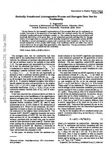
FIG. 1: Percentages of rejections of H0 using as discriminating statistics the fit of Volterra polynomials from 100 realisations for each of the three cases in the three panels, as indicated. Three types of surrogates are used in each test as shown in the legend (for STAP m = 5, p = 5). The vertical gray line distinguishes the linear from the nonlinear statistics.
STAP 20 30 40 50 60 number of polynomial terms i
(c) 10
6
AAFT IAAFT STAP
4
non−epileptic
8
time series of 2048 samples each and for each realisation we generate M = 40 surrogate data of each type. As discriminating statistics q i we choose the correlation coefficient (CC) of the fit with the series of Volterra polynomials of degree 2 and order v = 5. The polynomials for the first i terms, where i = 1, . . . , 5, are linear and for terms i = 6, . . . , 20 are nonlinear (see also [10]). To quantify the discrimination we use the significance |qi −hqi i| S i = 0 σi for each polynomial of i terms, where q0i is q
the statistic q i on the original data, hq i i and σqi are the mean and standard deviation of the statistic q i on the M surrogate data. The null hypothesis H0 is formally rejected at the 0.05 significance level when S > 1.96, under the assumption of normality for the statistic q, which turns out to hold in general. The percentages of rejections for each of the three systems are shown in Fig. 1. Very similar results were found when deciding the rejeci tion from the rank ordering of q0i , q1i , . . . , qM . For the linear statistics, STAP gives consistently and correctly no rejections, i.e. unbiased match of the linear correlations, whereas AAFT and IAAFT give very large percentages of rejections for all but the first case where AAFT gives about 5% rejections, as expected. For IAAFT, the rejections occur because σqi is very small (10 to 20 times smaller than for AAFT and STAP), though the bias q0i − hq i i is smaller than for STAP.
S
2 50 40 epileptic
30 20 10 0
10
20 30 40 50 number of polynomial terms i
60
FIG. 2: (a) The correlation coefficient of the fit with Volterra polynomials on the original normal EEG data (black line) and 40 AAFT, IAAFT and STAP surrogates (gray lines) in the three panels, as indicated (for STAP m = 10, p = 10). (b) The same as in (a) but for the epileptic EEG. (c) The significance for the fits in (a) (upper panel) and in (b) (lower panel) . The vertical lines in the plots distinguish the linear from the nonlinear polynomials.
For the nonlinear statistics, the feature of the linear statistics persists for the two first systems (consistent with H0 ) and for all three algorithms, i.e. correctly no rejections with STAP and erronous rejections with AAFT and IAAFT. We cannot explain why the polynomial fit for the IAAFT surrogates improves with the addition of nonlinear terms (see Fig. 1). For the nonlinear system, STAP properly converges with the addition of few non-
4 linear terms to the correct 100% rejection level, which AAFT and IAAFT possessed already with linear statistics. Next, we verify the three algorithms on two human EEG data sets, one recorded many hours before an epileptic seizure accounting for normal brain activity and another recorded during an epileptic seizure. The epileptic EEG seems to exhibit a pattern of oscillations indicating a more deterministic character than the non-epileptic EEG, and this constitutes a well established result in physiology. This is demonstrated also with the fit of Volterra polynomials in Fig. 2. The fit improves with the inclusion of the first nonlinear terms for the epileptic EEG but not for the non-epileptic EEG. These findings are confirmed statistically by the test with STAP surrogate data while the results of the test with AAFT and IAAFT are more or less confusing. In particular, the H0 on the normal EEG is erroneously rejected with AAFT because the difference in the fit between original and surrogate data is about the same for the linear and nonlinear polynomials (see Fig. 2a and c). The same test result is obtained with IAAFT for large nonlinear polynomials, whereas again there is significant difference in the linear fits between original and IAAFT surrogates (not easily discernible as both bias and variance are very small). Using STAP surrogates, the H0 is not rejected for both linear and nonlinear fits. For the epileptic EEG, there is again a clear difference in the linear fit between original data and AAFT surrogates and a smaller but equally significant difference between original data and IAAFT surrogates (see Fig. 2b and c). The significance S for both AAFT and IAAFT increases with the addition of the first couple of nonlinear terms, much more for IAAFT due to the small
variance of CC. However, the deviation in the linear fit does not support reliable rejection of H0 . On the other hand, using STAP surrogates, the H0 is properly rejected only for the nonlinear statistics and with high confidence (S < 2 for the linear fit and S ≃ 5 for the nonlinear fit). In general, the test with STAP surrogates tends to be more conservative, i.e. small discriminations are found less significant, as the data size decreases. For example, the test on 296 sunspot samples (for which a small leap of the polynomial fit with the addition of nonlinear terms was observed) gave rejection of H0 for AAFT and IAAFT but not for STAP (not shown here, see also [10]). However, this should not be considered as a drawback of the STAP algorithm, as one expects that the power of the test reduces with the decrease of data size. A new algorithm that generates surrogate data for the test for nonlinearity has been presented, called statically transformed autoregressive process (STAP). The key feature of STAP is that it finds analytically the autocorrelation of an appropriate underlying normal process for the test. This is the main difference of the STAP algorithm from the corrected AAFT (CAAFT) algorithm, where the autocorrelation is estimated numerically. Both CAAFT and STAP algorithms do not suffer from the severe drawback of the AAFT algorithm, i.e. bias in the match of the original autocorrelation. The AAFT algorithm is essentially impractical for real applications because it favours the rejection of H0 as a result of the bias in the autocorrelation. From the numerical simulations, it turns out that the IAAFT algortihm may also give small bias in the linear correlations, favouring also the rejection of H0 . On the other hand, the STAP algorithm performs properly and gives reliable rejections of H0 , only whenever this appears to be the case.
[1] H. Kantz and T. Schreiber, Nonlinear Time Series Analysis (Cambridge University Press, Cambridge, 1997). [2] C. Diks, Nonlinear Time Series Analysis: Methods and Applications (World Scientific, 2000). [3] T. Schreiber and A. Schmitz, Physica D 142, 346 (2000). [4] D. Kugiumtzis, in Modelling and Forecasting Financial Data, Techniques of Nonlinear Dynamics, edited by A. Soofi and C. Cao (Kwyer Academic Publishers, 2002), chap. 12. [5] D. Kugiumtzis, Internat. J. Bifur. Chaos Appl. Sci. Engrg. 11, 1881 (2001). [6] J. Theiler, S. Eubank, A. Longtin, and B. Galdrikian, Physica D 58, 77 (1992). [7] D. Kugiumtzis, Phys. Rev. E 60, 2808 (1999). [8] T. Schreiber and A. Schmitz, Phys. Rev. Lett. 77, 635 (1996). [9] T. Schreiber, Phys. Rev. Lett. 80, 2105 (1998). [10] D. Kugiumtzis, Phys. Rev. E 62, 25 (2000). [11] A. Papoulis, Probability, Random Variables, and Stochastic Processes (McGraw-Hill, Inc., 1991), p. 113, 3rd ed. [12] N. Johnson and S. Kotz, Distributions in Statistics, Continuous Multivariate Distributions (John Wiley and Sons, 1972), chap. 34, p. 15, Wiley Series in Probability and Mathematical Statistics.
[13] A. Der Kiureghian and P.-L. Liu, J. Eng. Mech. 112, 85 (1986). [14] C. D. Elphinstone, Comm. Statist. Theory Methods 12, 161 (1983). [15] D. M. Hawkins, Comput. Statist. 9, 233 (1994). [16] T. P. Hutchinson and C. D. Lai, Continuous Bivariate Distributions Emphasising Applications (Rumsby Scientific Publishing, 1990). [17] N. M. Bhatt and P. H. Dave, J. Indian Statist. Assoc. 2, 177 (1964). [18] P. J. Brockwell and R. A. Davis, Time Series: Theory and Methods, Springer Series in Statistics (SpringerVerlag, New York, 1991). [19] O. E. R¨ ossler, Physics Letters A 57, 397 (1976). [20] Other model classes may give better approximations of g and should be investigated, but polynomials were used here to derive a simple analytic form for the transform of the autocorrelations. [21] We found thatPa robust way to achieve this is to compute the error τi=1 (rx (i) − rz j (i))2 for j = 1, . . . , K and τ = 1, . . . , τmax and then select the trial l that gives the minimum error most times, where τmax minimums are totally computed, each time over the K trials.