Available online at www.sciencedirect.com
Energy Procedia 8 (2011) 135–140
SiliconPV: 17-20 April 2011, Freiburg, Germany
Statistical Approach to the Description of Random Pyramid Surfaces using 3D Surface Profiles E. Wefringhausa*, C. Kesnara, M. Löhmannb a
International Solar Energy Research Center Konstanz, Rudolf-Diesel-Str. 15, 78467 Konstanz, Germany b RENA GmbH, Ob der Eck 5, 78148 Gütenbach, Germany
Abstract 3D surface profiles obtained from a variety of mono-crystalline wafers textured under different conditions were investigated. Topographical parameters taking single pyramids heights and distances into account were analysed with regard to their statistical distribution. The statistical analysis yielded appropriate distribution functions allowing for quantitative description and comparison of random pyramid surfaces.
© under responsibility of of SiliconPV 2011. © 2011 2011 Published Publishedby byElsevier ElsevierLtd. Ltd.Selection Selectionand/or and/orpeer-review peer-review under responsibility SiliconPV 2011. Keywords: Anisotropic texturing; random pyramids; topography; laser scanning microscope; distribution functions
1. Introduction In solar cell production anisotropic texturing of mono-crystalline wafers, resulting in random upright pyramids, is a standard technique. Most widely KOH/IPA is employed, but recently a lot of alternatives have been developed [1-4]. Light coupling and light trapping in textured wafers, and thus performance of solar cells, depend on surface topography. Surface topography, i.e. (uniformity of) pyramid coverage, pyramid density and pyramid height, is usually assessed by single, randomly taken SEM pictures. These pictures are compared in order to derive qualitative statements as “a more uniform pyramid geometry” [5] or very rough classifications as “inhomogeneous pyramidal texture with pyramid size 1-6 μm” [6]. Mäckel et al. calculated “mean pyramid base length” from SEM pictures [7]. Souren et al. used AFM and LSM to calculate roughness parameters from measured height data [8]. The scope of this work was to define additional parameters which describe the surface characteristics from the statistical point of view.
* Corresponding author. Tel.: +49-7531-36183-21; fax: +49-7531-36183-11; E-mail address:
[email protected].
1876–6102 © 2011 Published by Elsevier Ltd. Selection and/or peer-review under responsibility of SiliconPV 2011. doi:10.1016/j.egypro.2011.06.114
136
E. Wefringhaus et al. / Energy Procedia 8 (2011) 135–140
2. Methods Figure 1 outlines how 3D surface data were generated, handled and evaluated. Applying different textures (2.1) Determination of surface profiles by measuring confocal laser scanning microscope (2.2) Calculation of pyramid height / distances and derived parameters by MountainsMap (2.3)
Evaluation of parameter statistics by EasyFit (2.4)
Fig. 1. Data generation, handling and evaluation.
2.1. Textures 20 wafers were taken from different experiments to generate a variety of different surfaces regarding pyramid size, distances and distribution. Textures were carried out using different pre-cleaning steps (no pre-cleaning, O3, SC1) and processes (standard KOH/IPA as well as alternative processes [3] and RENA monoTEX). 2.2. Determination of surface profiles 3D surface profiles were obtained by means of a measuring confocal laser scanning microscope (mcLSM) using an Olympus LEXT OLS4000 [9]. The edge length of the obtained pictures was 128 µm with a resolution of 1024x1024 pixels. 2.3. Processing of surface profiles and generation of topographical parameters The 3D surface profiles were transformed using an algorithm written in MountainsMap software. The raw height layer was filtered according to ISO/DIS 25178 [10, 11]. Furthermore a surface tilt correction was applied. Motifs (the pyramids) were separated using watershed algorithm. For statistical evaluation open motifs appearing at the edge of the pictures were excluded. A typical raw profile and a segmented profile are shown in Figure 2. From (x,y,z)-coordinates of motif peaks (pyramid tips) topographical parameters are derived describing the random pyramid surface (Table 1). 2.4. Evaluation of topographical parameter statistics The characterisation of mcLSM pictures by MountainsMap results in n data for each topographical parameter (see Table 1), where n is the number of motifs (pyramids) (e.g. 427 in Figure 2). Analysing the data parameter-wise by descriptive statistics yields median (and other quantiles), skewness S, and kurtosis K (compare [8]). Since each parameter is greater than zero per definition, data can obviously not be normally distributed. In order to find an appropriate distribution function, data were analysed by the maximum likelihood method using the software EasyFit. 37 bounded, non-negative distributions were considered and ranked according to significance using Kolmogorow-Smirnow, Anderson-Darling, and Chi-square tests, respectively.
137
E. Wefringhaus et al. / Energy Procedia 8 (2011) 135–140
0
0
20
40
60
80
100
120 μm
μm 9
10 20
8
30
7
40
6
50 60
5
70
4
80 90
3
100
2
110
1
120
0
μm
Number of motifs
427
Fig. 2. Raw height profile obtained from mcLSM (left side) and watershed segmented surface after applying filters and surface tilt correction (right side). The + signs mark peaks (pyramid tips) and the black lines the boundaries to adjacent motifs (pyramids). Table 1. Topographical parameters describing random pyramid surfaces generated by MountainsMap (top) and topographical parameters derived herefrom (bottom). “Idealities” should approach 1 in case of an ideal texture with uniform pyramids. Name
Explanation
Abbreviation
Height 1
Height between highest saddle point and peak (pyramid tip)
H
Height 2
Height of peak (pyramid) from the lowest point of the surface
Z
Coflatness
Maximum vertical distance between the pyramid tip and the tips of adjacent pyramids
CF
Min Pitch / Pitch / Max Pitch /
Minimum / mean / maximum horizontal distance between the pyramid tip and the tips of adjacent pyramids
MinP / P / MaxP
Base length
Pyramid base length calculated from Z: a (Z) = 1.414 Z
a
Ideality 1
MinPitch divided by base length a (Z)
MinP/a
Ideality 2
Height 1 divided by height 2
H/Z
3. Results Table 2 summarizes the results of the statistical analysis. Details, explaining the method of ranking the distribution functions, are depicted in the appendix. Appropriate distribution functions were found for all defined parameters with the exception of Minimum Pitch. Results are exemplarily illustrated in Figure 3. Table 2. Appropriate distribution functions for defined topographical parameters (in brackets: number of distribution parameters). Parameter
Appropriate distribution function
Distribution to be rejected (in two out of three tests, p = 0.05)
Height 1, H
Fatigue life (3P)
2 of 20 times
Height 2, Z
Johnson SB (4P) / Burr (4P)
0 of 11 times (9 times not applicable) / 1 of 20 times
Coflatness, CF
Johnson SB (4P)
0 of 20 times
Minimum Pitch, MinP
No appropriate distribution found, but best fitting: Dagum (4P), Inverse Gaussian (3P), Frechet (3P)
Pitch, P
Johnson SB (4P)
2 of 18 times (2 times not applicable)
Maximum Pitch, MaxP
Generalized Extreme Value (3P)
0 of 20 times
Ideality 1, minP/a
Fatigue life (3P)
4 of 20 times
Ideality 2, H/Z
Johnson SB (4P)
4 of 20 times
138
E. Wefringhaus et al. / Energy Procedia 8 (2011) 135–140
0,4
0,14
0,36
0,12
0,32
0,1
0,28 0,24
0,08
0,2 0,16
0,06
0,12
0,04
0,08
0,02
0,04 0
1
2
3
0
4
4
6
H [μm] 0,11 0,1 0,09 0,08 0,07 0,06 0,05 0,04 0,03 0,02 0,01 0
2
4
6
0,22 0,2 0,18 0,16 0,14 0,12 0,1 0,08 0,06 0,04 0,02 0
8
1
2
3
4
5
8
10
0,1 0,09 0,08 0,07 0,06 0,05 0,04 0,03 0,02
2
4
6
8
0,01 0
P [μm] 0,12 0,11 0,1 0,09 0,08 0,07 0,06 0,05 0,04 0,03 0,02 0,01 0
10
MinP [μm]
CF [μm] 0,12 0,11 0,1 0,09 0,08 0,07 0,06 0,05 0,04 0,03 0,02 0,01 0
8
Z [μm]
0,1
0,2
MinP / a
2
4
6
MaxP [μm]
0,3
0,24 0,22 0,2 0,18 0,16 0,14 0,12 0,1 0,08 0,06 0,04 0,02 0
0,1
0,2
0,3
0,4
H/Z
Fig. 3. Probability densities for height H (fatigue life distribution), height Z (Burr distribution), coflatness CF (Johnson SB distribution), minimum pitch MinP (Dagum distribution), pitch P (Johnson SB distribution), maximum pitch MaxP (generalized extreme value distribution), ideality MinP/a (fatigue life distribution), and ideality H/Z (Johnson SB distribution) for a sample textured by KOH/IPA.
E. Wefringhaus et al. / Energy Procedia 8 (2011) 135–140
4. Outlook Distribution functions found for the different defined topographical parameters allow for quantitative description and comparison of random pyramid surfaces. Further investigations are ongoing with respect to Classification of textured wafers according to process conditions, Correlation of distribution function parameters and roughness parameters, Correlation of distribution function parameters and wafer reflection, Correlation of distribution function parameters and solar cell performance, Moreover, statistical methods describing the spatial distribution of pyramids (e.g. by dispersion indices) are under investigation.
References [1] Birmann K, Zimmer M, Rentsch J. Fast alkaline etching of monocrystalline wafers in KOH/CHX. Proc. 23rd EU PVSEC, Valencia, Spain; 1-5 September 2008, p. 1608-11. [2] Wefringhaus E, Helfricht A. KOH/surfactant as an alternative to KOH/IPA for texturisation of monocrystalline silicon. Proc. 24th EU PVSEC, Hamburg, Germany; 21-25 September 2009, p. 1860-2. [3] Krümberg J, Melnyk I, Schmidt M, Michel M, Fidler T, Kagerer M et al. New innovative alkaline texturing process for CZ silicon wafers. Proc. 24th EU PVSEC, Hamburg, Germany; 21-25 September 2009, p. 1748-50. [4] Moynihan M, O´Connor C, Barr B, Tiffany S, Braun W, Allardyce G et al. IPA free texturing of mono-crystalline solar cells. Proc. 25th EU PVSEC / 5th WC PEC, Valencia, Spain; 6-10 September 2010, p. 1332-36. [5] Vazsonyi E, De Clercq K, Einhaus R, Van Kerschaver E, Said K, Poortmans J et al. Improved anisotropic etching process for industrial texturing of silicon solar cells. Solar Energy Materials & Solar Cells 1999; 57: 179-88. [6] Ximello N, Haverkamp H, Hahn G. Influence of pyramid size of chemically textured silicon wafers on the characteristics of industrial solar cells. Proc. 25th EU PVSEC / 5th WC PEC, Valencia, Spain; 6-10 September 2010, p. 1761-4. [7] Mäckel H, Cambre DM, Zaldo C, Albella JM, Sánchez S, Vázquez C et al. Characterisation of monocrystalline silicon texture using optical reflectance patterns. Proc. 23rd EU PVSEC, Valencia, Spain; 1-5 September 2008, p. 1160-3. [8] Souren FMM, Van de Sanden MCM, Kessels WMM, Rentsch J. Quantitative characterization of dry textured surfaces. Proc. 24th EU PVSEC,. Hamburg, Germany; 21-25 September 2009, p. 1909-13. [9] Fabich M. Advanced confocal laser scanning microscopy. Physics´ Best 2010; Special Issue: 18-21. [10] ISO/DIS 25178-2:2008. Geometrical product specifications (GPS) – surface texture: Areal – Part 2: Terms. definitions and surface texture parameters. [11] ISO/DIS 25178-3:2008. Geometrical product specifications (GPS) – surface texture: Areal – Part 3: Specification operators.
139
140
E. Wefringhaus et al. / Energy Procedia 8 (2011) 135–140
Appendix A. Method of ranking distribution functions according to significance (example: Pitch P). Distribution
Kolmogorow Smirnow
Anderson Darling
SoR*
appl.**
mean rank
SoR*
appl.**
mean rank
Chi-square SoR*
appl.**
mean rank
Beta
156
20
7.80
90
20
4.50
138
20
6.90
Burr (4P)
198
20
9.90
159
20
7.95
189
20
9.45
Chi-Squared (2P)
600
20
30.00
556
20
27.80
510
20
25.50
Dagum (4P)
289
20
14.45
249
20
12.45
243
20
12.15
Erlang (3P)
399
20
19.95
366
20
18.30
283
20
14.15
Exponential (2P)
612
20
30.60
572
20
28.60
517
20
25.85
Fatigue Life (3P)
209
20
10.45
177
20
8.85
170
20
8.50
Frechet (3P)
468
20
23.40
423
20
21.15
155
10
15.50
Gamma (3P)
193
20
9.65
157
20
7.85
199
20
9.95
Gen. Extreme Value
148
20
7.40
142
20
7.10
157
19
8.26
Gen. Gamma (4P)
171
20
8.55
98
20
4.90
142
20
7.10
Gen. Logistic
358
20
17.90
350
20
17.50
334
20
16.70
Gen. Pareto
328
20
16.40
594
20
29.70
Inv. Gaussian (3P)
390
20
19.50
362
20
18.10
296
20
14.80
Johnson SB
58
18
3.22
79
18
4.39
117
16
7.31
Kumaraswamy
256
20
12.80
221
20
11.05
259
20
12.95
Log-Gamma
166
6
27.67
149
6
24.83
146
6
24.33
Log-Logistic (3P)
317
20
15.85
319
20
15.95
295
20
14.75
Log-Pearson 3
172
20
8.60
164
20
8.20
166
19
8.74
Lognormal (3P)
212
20
10.60
198
20
9.90
161
20
8.05
Nakagami
300
20
15.00
287
20
14.35
254
20
12.70
Pearson 5 (3P)
242
20
12.10
243
20
12.15
195
20
9.75
Pearson 6 (4P)
224
20
11.20
198
20
9.90
184
20
9.20
Pert
349
20
17.45
327
20
16.35
329
20
16.45
Phased Bi-Expon.
606
20
30.30
607
20
30.35
574
20
28.70
Phased Bi-Weibull
651
19
34.26
647
19
34.05
412
13
31.69
Power Function
589
20
29.45
552
20
27.60
308
13
23.69
Rayleigh (2P)
409
20
20.45
373
20
18.65
336
20
16.80
Reciprocal
634
20
31.70
600
20
30.00
538
20
26.90
Rice
431
20
21.55
416
20
20.80
377
20
18.85
Wakeby
63
20
3.15
480
20
24.00
8
1
8.00
Weibull (3P)
230
20
11.50
208
20
10.40
254
20
12.70
0
* SoR = Sum of Ranks, ** appl. = distribution applicable in n out of 20 cases (pictures/textures); five clearly non-fitting distributions were excluded from table due to space constraints: Levy (2P), Pareto, Pareto 2, Triangular, and Uniform.