such as MINITAB are particularly useful for routine analysis of statistical data, many ... instruction in statistical analysis techniques using SPSS for Windows.
Statistical Computing Using SPSS: A Guide for Students
Rachel A. Heath Newcastle, NSW Australia
R. A. Heath, 2014
1
Preface This manual contains information and examples illustrating the use of the Windows Version 9 of the SPSS Statistical Data Analysis Package for the analysis of psychological data. Although other statistical packages such as MINITAB are particularly useful for routine analysis of statistical data, many psychologists and social scientists make extensive use of sophisticated mainframe packages, especially SPSS. The current version of SPSS contains sufficient analytical tools to satisfy the most discerning data analyst. SPSS's graphics features in the Windows environment are very comprehensive and easy to use. Their flexibility encourages students to use contemporary Exploratory Data Analysis (EDA) techniques to examine their data prior to data analysis to assist in the choice of an appropriate data analysis procedure. The graphics tools permit a detailed appraisal of the analysis once it has been performed. This is an advantage since a common procedure in the analysis of social data sets is to ignore the important descriptive and graphical features of the data set prior to reporting the results of the analysis. In this version of the Guide we concentrate on the SPSS Menu commands rather than the equivalent syntax commands which can also be used in a mainframe, offline computing environment. The first section material analyzed in this manual derives directly from Howell's (1992) third edition of his popular textbook Statistical Methods For Psychology. The examples are chosen from Chapters 7, 9, 10, 11, 12, 13, 14, 15, 16, 17 and 18 in Howell (1992). A section on Logistic Regression in Chapter 6 is based on Chapter 15 in the Fourth Edition of Howell (1997). Readers are encouraged to apply the techniques in this Guide to the different examples presented in Howell (1997). Common exercises from both editions of Howell's’book are indicated. In the early chapters, the example analyses derive from the Computer Exercises at the end of these chapters. Analyses of the worked out examples in the text are provided for the later chapters. It is expected that students will also want to practice their skills analyzing real data which they collect themselves. The analyses reported in this guide should serve as useful models for the detailed statistical analysis of these data sets. Each analysis follows the strategy of (1) exploring the data characteristics using EDA, (2) computing an appropriate statistical analysis, and (3) evaluating the analysis using such techniques as residual and fit analysis. It is recommended that students use this procedure as a guide for their analysis of real data sets, especially when the statistical techniques are likely to produce misleading results if there are systematic deviations from the basic statistical model assumptions, or if there are undesirable effects of outliers. The analyses reported in this Student Guide are organized around the data sets provided with Howell's book. The reader should refer to the Appendix in Howell (1992) for a detailed description of these data sets. This Guide contains annotated SPSS output that was obtained by analyzing the appropriate Worksheet files. This manual is organized into Chapters that can be used in separate Tutorial sessions which provide instruction in statistical analysis techniques using SPSS for Windows. These Chapters cover the following material: Chapter 1: Hypothesis Tests Applied to Means Chapter 2: Correlation and Regression Chapter 3: Simple Analysis of Variance and Multiple Comparisons among Treatment Means Chapter 4: Factorial Analysis of Variance Chapter 5: Repeated Measures Designs Chapter 6: Multiple Linear Regression and Applications, including Logistic Regression Chapter 7: Analysis of Variance and Covariance as General Linear Models Chapter 8: Nonparametric Tests Chapter 9: The Log-Linear Model
2
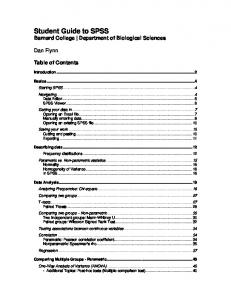
How to Use This Student Guide The SPSS applications described in this Guide follow the examples in successive chapters of Howell (1992). For this reason they do not necessarily follow the type of sequential development found, for example, in books that concentrate on the SPSS commands themselves, without any specific application in mind. For this reason, it is essential that the user have a copy of Howell (1992) on hand since much of the detailed explanation of the statistical procedures, which is contained in Howell's book, is omitted here. When appropriate we indicate the Menu commands using Bold Times Roman Font, each submenu being separated by an arrow => e.g. Analyze => Descriptive Statistics => Frequencies We omit the detailed menu screen shots from this Manual to save space since we assume that the user will make full use of the SPSS HELP facility as well as guidance from the various SPSS For Windows Reference Manuals that are available. The SPSS output, which also appears on the Navigator Output Window, is printed in Courier Font with Bold being used to highlight significant features of the Output, e.g. Variable DEPRESST By Variable GROUP Analysis of Variance Sum of Mean F F Source D.F. Squares Squares Ratio Prob Between Groups 2 349.7 174.9 1.95 0.144 Within Groups 372 33435.9 89.9 Total 374 33785.6 or in Object Tables such as Case Processing Summary
IQ
Valid N Percent 88 100.0%
Cases Missing N Percent 0 .0%
Total N Percent 88 100.0%
There will be the usual number of unclear statements and errors, for which I am entirely responsible. I would appreciate receiving feedback and corrections from the users of this Guide. If, convenient, please send them to me at the email address on the cover page. I hope you find this Manual helpful, especially since it is only when you have the opportunity to apply statistical procedures using modern computing techniques, that your understanding of the basic statistical principles that guide most of social science research can be enhanced. It is very important that you supplement your practical knowledge of statistical procedures with a firm foundation in research methodology. For this reason, I recommend that you read any good book on research methodology for social scientists, for example, the very comprehensive and readable book entitled by Christensen (1994). References: Christensen, L.B. (1994). Experimental Methodology. Boston: Allyn and Bacon. Howell, D.C. (1992). Statistical methods for psychology (3rd Edition). Belmont, CA: Duxbury Press. Howell, D.C. (1997). Statistical methods for psychology (4th Edition). Belmont, CA: Duxbury Press.
3
CHAPTER 1 Hypothesis Tests Applied To Means The analysis techniques described in this Chapter are based on material in Chapter 7 of Howell (1992). In addition to providing revision of basic statistical hypothesis testing procedures, it allows students to familiarize themselves with the SPSS for Windows statistical analysis package and especially the use of menu procedures for executing SPSS commands. These procedures are described in more detail in Appendix B.
The SPSS Worksheet Data are stored in the SPSS Worksheet which is organized in terms of columns, each column representing a data variable. In many social science applications the rows of the Worksheet represent subjects. Columns should be labeled by clicking the mouse button on any data value in that column and then using the following pulldown menu command: Data => Define Variable Column names can be up to 8 characters long and should begin with a letter. Example 1: Exercise Howell (1992) Chapter 7.45 [Ex. 7.36 in Howell(1997)] In this example we compute a single sample T-test on the data file ADD.DAT. The corresponding Worksheet is ADD.SAV It should be noted that a MINITAB Worksheet file can be read into SPSS by first reading it into MINITAB using the Open Worksheet menu command. Use the Edit menu to Select All the data cells (but not the variable names) and then select Edit => Copy Cells. Now open the SPSS Worksheet and then click on the top left most data cell. Use the Edit => Paste command to insert the data in the Worksheet. You will need to define the Variable names using the SPSS procedure. Firstly we perform Exploratory Data Analysis (EDA) for the IQ measure using the SPSS command Analyze => Descriptive Statistics => Frequencies This command yields a command box which allows you to select the variable(s) to be analyzed (IQ in this case) and the various types of descriptive statistics, frequency tables and histograms (with best fitting normal distribution) which you might require. The output is generated in a different window called the Output Window. You can save the contents of this Window in an SPSS Output file addiqfreq.spo The easiest way to insert the SPSS results into a Microsoft Word (say) report is to click the mouse on the item(s) you wish to insert and then use the menu command Edit => Copy Objects in the SPSS Output Window and the Edit => Paste command in Word. In the example below we have copied the descriptive statistics, frequency chart and the histogram. The descriptive statistics table is too wide to save in this document, but by double-clicking on it in the Output Window you can produce a scrollbar chart that is easy to read. The following tables contain a comprehensive list of Descriptive Statistics, including the mean, median, mode, standard deviation, variance, skewness, kurtosis, range, the minimum and maximum observations and the 25th, 50th and 75th percentiles. It is worth noting that in the case of skewness and kurtosis the standard errors are provided. Under the null hypotheses of no departure from the skewness and kurtosis values characteristic of a normal distribution (set equal to 0), we discover that the approximate 95% confidence intervals for these statistics (2.0 times the standard error below the estimate up to 2.0 times the standard error above the estimate) contain the population values equal to 0. Hence we have no statistical evidence to reject the null hypotheses that the skewness and kurtosis values equal 0. These observations are confirmed by the good fit of the superimposed normal distribution in the following histogram of IQ scores.
4
Statistics IQ N
Valid Missing
Statistic Statistic Statistic Std. Error Statistic Statistic Statistic Statistic Statistic Std. Error Statistic Std. Error Statistic Statistic Statistic Statistic Statistic Statistic
Mean Median Mode Std. Deviation Variance Skewness Kurtosis Range Minimum Maximum Percentiles
25.0000 50.0000 75.0000
88 0 100.2614 1.3842 100.0000 95.00 12.9850 168.6091 .394 .257 -.163 .508 62.00 75.00 137.00 90.2500 100.0000 108.7500
Histogram 14 12 10 8
Frequency
6 4 Std. Dev = 12.98
2
Mean = 100.3 N = 88.00
0 75.0
85.0 80.0
95.0 90.0
105.0
100.0
115.0
110.0
125.0
120.0
135.0
130.0
IQ The next table contains a detailed frequency table which orders the observations from smallest to largest then provides the frequency, percentage and cumulative percentage for each of the observations in the data set. For example, for an IQ equal to 100 we have three observations constituting 3.4% of the total sample. 51.1% of the sample have an IQ of 100 or less.
5
IQ
Valid
Total
75.00 79.00 81.00 82.00 83.00 84.00 85.00 86.00 88.00 89.00 90.00 91.00 92.00 93.00 94.00 95.00 96.00 97.00 98.00 99.00 100.00 101.00 102.00 103.00 104.00 105.00 106.00 107.00 108.00 109.00 110.00 111.00 112.00 114.00 115.00 118.00 120.00 121.00 127.00 128.00 131.00 137.00 Total
Frequency 1 1 2 3 2 2 3 2 3 2 1 3 2 2 1 6 2 1 2 1 3 2 3 2 1 3 4 3 3 3 1 4 1 1 2 3 2 1 1 1 1 1 88 88
Percent 1.1 1.1 2.3 3.4 2.3 2.3 3.4 2.3 3.4 2.3 1.1 3.4 2.3 2.3 1.1 6.8 2.3 1.1 2.3 1.1 3.4 2.3 3.4 2.3 1.1 3.4 4.5 3.4 3.4 3.4 1.1 4.5 1.1 1.1 2.3 3.4 2.3 1.1 1.1 1.1 1.1 1.1 100.0 100.0
Valid Percent 1.1 1.1 2.3 3.4 2.3 2.3 3.4 2.3 3.4 2.3 1.1 3.4 2.3 2.3 1.1 6.8 2.3 1.1 2.3 1.1 3.4 2.3 3.4 2.3 1.1 3.4 4.5 3.4 3.4 3.4 1.1 4.5 1.1 1.1 2.3 3.4 2.3 1.1 1.1 1.1 1.1 1.1 100.0
Cumulative Percent 1.1 2.3 4.5 8.0 10.2 12.5 15.9 18.2 21.6 23.9 25.0 28.4 30.7 33.0 34.1 40.9 43.2 44.3 46.6 47.7 51.1 53.4 56.8 59.1 60.2 63.6 68.2 71.6 75.0 78.4 79.5 84.1 85.2 86.4 88.6 92.0 94.3 95.5 96.6 97.7 98.9 100.0
6
It is worth noting that the Output file can be edited using the Insert menu options. You can insert headers, titles, explanatory text etc. Furthermore you can export the contents of this file (Using the Export pulldown menu) using either text or HTML format, the latter being used to present information on the World Wide Web. The SPSS Menu command Analyze => Descriptive Statistics => Explore allows us to compute exploratory data analysis statistics and plots, such as the 95% confidence intervals for both the Mean and the Median, together with a stem-and-leaf plot. It is worth noting that you can save standardized versions of each of your data columns by clicking on the “Save standardized values as variables” box in the Dialog Box. You can reselect variables by first clicking the mouse on the Reset button in the Dialog Box. We obtain the following descriptive statistics: Case Processing Summary
IQ
Valid N Percent 88 100.0%
Cases Missing N Percent 0 .0%
N
Total Percent 88 100.0%
Descriptives
IQ
Mean 95% Confidence Interval for Mean
Statistic 100.2614 Lower Bound Upper Bound
Std. Error 1.3842
97.5101 103.0126
5% Trimmed Mean 99.7828 Median Variance Std. Deviation Minimum Maximum Range Interquartile Range Skewness Kurtosis
100.0000 168.609 12.9850 75.00 137.00 62.00 18.5000 .394 -.163
.257 .508
The above table provides the basic descriptive statistics for the IQ variable in a slightly different way to the previous command. For example, since the sample mean of 100.26 lies in the 95% confidence interval for the population mean (97.5101, 103.0126) we are justified in assuming that the population mean is 100. As we saw previously, the low values of skewness and kurtosis are consistent with the hypothesis that the IQ scores are normally distributed. The following table contains a Stem and Leaf plot in the form of a histogram, which once again confirms the normality assumption.
7
IQ Stem-and-Leaf Plot Frequency
Stem &
2.00 7 19.00 8 21.00 9 27.00 10 12.00 11 5.00 12 1.00 13 1.00 Extremes Stem width: Each leaf:
. . . . . . .
Leaf 59 1122233445556688899 011122334555555667889 000112223345556666777888999 011112455888 00178 1 (>=137)
10.00 1 case(s)
150 140 27
130 120 110 100 90 80 70 N=
88
IQ
The above figure shows the box-plot for the IQ variable. As you can see by the labeled circle, observation number 27 is an outlier that should be examined carefully and perhaps removed from the data set prior to further analysis. Otherwise the distribution is quite symmetric and well behaved.
Testing the Normality Assumption We can test whether a data set is normally distributed by using the SPSS Menu command Graphs => P-P and then selecting the normal distribution and keeping the remaining values of the dialog box at their current (default) values. We obtain the following Normal P-P and Detrended Normal P-P graphs:
8
Normal P-P Plot of IQ 1.00
.75
Expected Cum Prob
.50
.25
0.00 0.00
.25
.50
.75
1.00
Observed Cum Prob
Detrended Normal P-P Plot of IQ .06
.04
.02
0.00
-.02
-.04 -.2
0.0
.2
.4
.6
.8
1.0
1.2
Observed Cum Prob Since the data points in the Normal P-P plot lie close to the best fitting straight line, this result indicates that the normal assumption is appropriate. This result is confirmed by the Detrended Normal P-P plot indicating that the observations are spread approximately equally on each side of the horizontal line which indicates zero deviation from normality. However there is a discernible inverted U trend between 0.0 and 0.6 on the Observed Cumulative Probability axis, that might suggest a departure from normality that is not easily detected by the current tests.
9
Computing a Single Sample t-Test Since the data are normally distributed, we can confidently compute a single sample t-test which tests the following Null (H0) and Research (H1) hypotheses (where IQ refers to the corresponding population mean): H0: IQ = 100 H1: IQ 100 Use the SPSS Menu command Analyze => Compare Means => One-Sample T Test together with the associated dialog box (you need to set the Test value to 100) to compute the following output:
T-Test One-Sample Statistics
N IQ
88
Mean 100.2614
Std. Deviation 12.9850
Std. Error Mean 1.3842
One-Sample Test Test Value = 100
t IQ
df .189
87
Sig. (2-tailed) .851
95% Confidence Interval of the Difference Mean Difference Lower Upper .2614 -2.4899 3.0126
Since the p value of 0.851 is not less than 0.05, we do not reject H0: IQ=100. There is no evidence to support the research hypothesis that the population mean IQ is not equal to 100. That's a relief! We can also evaluate a one tailed (directional) research hypothesis such as H1: IQ > 100 by changing the confidence from 95 to 90 in the dialog box and then examining the Confidence Interval for the differences in means. Since the above table for the One-Sample Test shows that the standardized mean IQ, equal to 0, lies within the confidence interval, we cannot reject the Null Hypothesis.
Computing A Repeated Measures t-Test Example 2: Exercise H7.46 from Chapter 7 of Howell (1992) [Ex 7.37 in Howell(1997)] Firstly, we compute descriptive statistics for the variables 'ENGG' and 'GPA' using the SPSS Menu command Analyze => Descriptive Statistics => Explore The resulting output is contained in the following Table:
10
Descriptives
ENGG
Mean 95% Confidence Interval for Mean
Statistic 2.6591 Lower Bound Upper Bound
Std. Error .1008
2.4588 2.8594
5% Trimmed Mean 2.6894 Median Variance Std. Deviation
3.0000 .894 .9455
Minimum Maximum Range Interquartile Range
GPA
Skewness Kurtosis Mean 95% Confidence Interval for Mean
.00 4.00 4.00 1.0000 -.264 -.414 2.4563 Lower Bound Upper Bound
.257 .508 9.183E-02
2.2737 2.6388
5% Trimmed Mean 2.4746 Median Variance Std. Deviation Minimum Maximum Range Interquartile Range Skewness Kurtosis
2.6350 .742 .8614 .67 4.00 3.33 1.2500 -.352 -.649
.257 .508
In this case we obtain estimates of the Means, Medians, Trimmed Means (removes the top and bottom 5% of observations to minimize the effects of outliers), the Standard Deviations, Standard Errors of the Means, together with the Minima, Maxima and the first and third Quartiles (the 25-th and 75-th percentiles, respectively). The Skewness and Kurtosis measures are also presented. Since the Trimmed Means are close to the actual Means we do not suspect any outliers. We also notice that the Standard Deviations are comparable, suggesting that the homogeneity of variance assumption is tenable, i.e. we can pool the sample variances to estimate the population variance more accurately. Note that if this latter assumption is violated, the two-sample t-test can still be computed using SPSS since test statistics for both equal and unequal population variance are computed.
11
Firstly, we apply EDA to both samples separately using the SPSS Menu command Analyze => Descriptive Statistics => Explore which yields the following histograms, Normal P-P plots and BoxPlots. Histogram 40
Normal Q-Q Plot of ENGG 1.5
30
1.0 .5 0.0
20
Expected Normal
-.5
Frequency
10
-1.0 -1.5
Std. Dev = .95 Mean = 2.7
-2.0
N = 88.00
0 0.0
1.0
2.0
3.0
4.0
-2.5 -1
ENGG
0
1
2
3
4
5
Observed Value
Histogram
Normal Q-Q Plot of GPA
14
3
12 2
10 1
8 0
Frequency
4
Expected Normal
6
-1
Std. Dev = .86
2
Mean = 2.46
-2
N = 88.00
0 .75
1.25 1.00
1.75
1.50
2.25
2.00
2.75
2.50
3.25
3.00
3.75
3.50
-3
4.00
0
GPA
1
2
3
4
5
Observed Value 5
5
4
4
3
3 2
2 1
1 0
64
0
-1 N=
88
ENGG
N=
88
GPA
We can also obtain a statistical significance test for Normality using the Kolmogorov-Smirnov Test of goodness-of-fit as shown in the following Table.
12
Tests of Normality Kolmogorov-Smirnova Statistic df Sig. .209 88 .000 .100 88 .030
ENGG GPA
a. Lilliefors Significance Correction
It is clear that the Kolmogorov-Smirnov Normality Test is significant for each of these variables. We reject the normality assumption for ENGG using the Kolmogorov-Smirnov goodness-of-fit test (KS= 0.209, p < 0.001), although it is still evident that the distribution is unimodal and there is only one extreme outlier. We can still use the t-test since it is known to be quite robust especially if the equal variance assumption applies. For the variable 'GPA' we reject the Normality assumption (KS= 0.10, p = 0.03), although the distribution is unimodal. There is evidence for a substantial negative skew. Since the data are not normally distributed we could use a nonparametric test for two dependent samples, as described in Chapter 8 and repeated below. Before applying the Repeated Measures t-test, we will check to see whether the samples, 'ENGG' and 'GPA' are correlated. Firstly we graph a scatterplot using the SPSS Menu command Graphs => Scatter which yields the following graph
Correlation of ENGG and GPA in ADD.DAT 5
4
3
2
ENGG
1
0
-1 .5
1.0
1.5
2.0
2.5
3.0
3.5
4.0
4.5
GPA The above scattergram exhibits a moderate positive correlation between these two variables. In this example we have inserted a graph Title in the Dialog Box for this command. This correlation estimate is confirmed by the SPSS Menu command Analyze => Correlate => Bivariate
13
which, when the options for Pearson’s r, Kendall’s , and Spearman’s options are clicked in the Dialog Box, yields the following tables: Correlations
Pearson Correlation Sig. (2-tailed) N
ENGG 1.000 .839** . .000 88 88
ENGG GPA ENGG GPA ENGG GPA
GPA .839** 1.000 .000 . 88 88
**. Correlation is significant at the 0.01 level (2-tailed).
You will notice from the above table that the Pearson correlation coefficient equals 0.839, a statistically significant value, p< 0.001.
Nonparametric Correlations Correlations
Kendall's tau_b
Correlation Coefficient Sig. (2-tailed) N
Spearman's rho
Correlation Coefficient Sig. (2-tailed) N
ENGG GPA ENGG GPA ENGG GPA ENGG GPA ENGG GPA ENGG GPA
ENGG 1.000 .726** . .000 88 88 1.000 .834** . .000 88 88
GPA .726** 1.000 .000 . 88 88 .834** 1.000 .000 . 88 88
**. Correlation is significant at the .01 level (2-tailed).
The above table shows that both nonparametric correlation coefficients are statistically significant. Since the scores are correlated and the data are not normally distributed, we use the nonparametric Wilcoxon test provided by the SPSS Menu command Analyze => Nonparametric Tests => 2 Related Samples This yields the following tables:
14
Ranks Mean Rank
N GPA ENGG
Negative Ranks Positive Ranks Ties Total
52 17
a
b
Sum of Ranks
34.05
1770.50
37.91
644.50
19 c 88
a. GPA < ENGG b. GPA > ENGG c. ENGG = GPA
Test Statisticsb
Z Asymp. Sig. (2-tailed)
GPA ENGG -3.385a
Test Statisticsa
.001
a. Based on positive ranks. b. W ilcoxon Signed Ranks Test
GPA ENGG -4.093
Z Asymp. Sig. (2-tailed)
.000
a. Sign Test
In this case we reject H0 and conclude that there is a significant difference between the population medians for ENGG and GPA, using both the Wilcoxon Signed Ranks Test (z = -3.385, p= 0.001) and the Sign Test (z = -4.093, p< 0.001). We can confirm this analysis by using the parametric repeated measures t-test, using the SPSS Menu command Analyze => Compare Means => Paired-Samples T Test This command yields the following results:
T-Test Paired Samples Statistics
Pair 1
ENGG GPA
Mean 2.6591 2.4563
Std. Deviation .9455 .8614
N 88 88
Std. Error Mean .1008 9.183E-02
Paired Samples Correlations N Pair 1
ENGG & GPA
Correlation 88
.839
Sig. .000
15
Paired Samples Test
Paired Differences
Pair 1 ENGG GPA .2028
Mean Std. Deviation
.5188
Std. Error Mean
5.531E-02
95% Confidence Interval of the Difference
Lower Upper
t df Sig. (2-tailed)
9.292E-02 .3128 3.668 87 .000
The results in the above Table confirm our previous finding. In this case the degrees of freedom (df) equal 87 (i.e. N-1) so we state that t(87) = 3.668, p < 0.001. It is worthwhile noting that the hypothesised population mean difference when H0 is true (0), is not contained within the 95% confidence interval for the population mean (0.0093, 0.3128). Note that the scientific number notation E-02 means that the number before it has its decimal point moved two places to the left. E+02, on the other hand, means that the number before it has its decimal point moved two places to the right.
One-Way Between-Subjects Analysis of Variance Example 3.: Exercise H7.48 from Chapter 7 in Howell (1992) [Ex. 7.41 in Howell (1997)] This example employs a one-way Analysis of Variance (ANOVA) with an independent groups, or Between-Subjects, design using the data contained in the SPSS Worksheet MIREAULT.SAV. We compare the scores on Depression (depresst), Anxiety(anxt) and Global Symptom Index T (gsit) for subjects from intact families and those who have experienced parental loss through either death or divorce. Before running the ANOVA, we perform Exploratory Data Analysis (EDA) on these variables using the SPSS menu command Analyze => Descriptive Statistics => Explore When this command is run we obtain the following descriptive statistics, normality test and histogram.
Case Processing Summar y Cases Valid N
Missing
DEPRESST
375
Percent 98.4%
ANXT
375
GSIT
375
N
Total
6
Percent 1.6%
98.4%
6
98.4%
6
N 381
Percent 100.0%
1.6%
381
100.0%
1.6%
381
100.0%
Tests of Normality Kolmogorov-Smirnov a DEPRESST
Statistic .082
df
Sig. 375
.000
ANXT
.057
375
.006
GSIT
.048
375
.036
a. Lilliefors Significance Correction
16
It is clear from the Normality tests that none of these distributions is normal. This can be verified by examining the following histograms.
Histogram 80
60
Frequency
40
20 Std. Dev = 9.50 Mean = 60.9 N = 375.00
0 40.0 45.0 50.0 55.0 60.0 65.0 70.0 75.0 80.0
DEPRESST
Histogram
Histogram
120
100
100 80
80 60
60 40
Std. Dev = 9.63
20
Mean = 60.2 N = 375.00
0 40.0
50.0 45.0
ANXT
60.0 55.0
70.0 65.0
80.0 75.0
Frequency
Frequency
40
20
Std. Dev = 9.24 Mean = 62.0 N = 375.00
0 35.0
45.0 40.0
55.0 50.0
65.0 60.0
75.0 70.0
80.0
GSIT
The distribution for GSIT is slightly negatively skewed with a few outliers. In real data sets these outliers are worth close inspection. Although the distribution is unimodal, it is clearly non-normal. If there are equal numbers of observations in each experimental treatment, the robustness of Analysis of Variance allows us to interpret the test statistics, despite these departures from the normality assumption. The following Table provides a detailed account of the descriptive statistics for each variable.
17
Descriptives
DEPRESST
Statistic 60.9387
Mean 95% Conf idence Interval for Mean
Lower Bound
59.9736
Upper Bound
61.9038
5% Trimmed Mean
60.9348
Median
60.0000
Variance
90.336
Std. Deviation
9.5045
Minimum
42.00
Maximum
80.00
Range
38.00
Interquartile Range
ANXT
14.0000
Skewness
-.092
.126
Kurtosis
-.426
.251
60.1547
.4971
Mean 95% Conf idence Interval for Mean
Lower Bound
59.1773
Upper Bound
61.1320
5% Trimmed Mean
60.2467
Median
60.0000
Variance
92.650
Std. Deviation
9.6255
Minimum
38.00
Maximum
80.00
Range
42.00
Interquartile Range
GSIT
Std. Error .4908
13.0000
Skewness
-.122
Kurtosis
-.298
.251
62.0453
.4772
Mean 95% Conf idence Interval for Mean 5% Trimmed Mean
Lower Bound
61.1069
Upper Bound
62.9838 62.1941
Median
61.0000
Variance
85.412
Std. Deviation
9.2419
Minimum
34.00
Maximum
80.00
Range
46.00
Interquartile Range
.126
12.0000
Skewness
-.175
.126
Kurtosis
.156
.251
18
We will employ the parametric independent groups one-way ANOVA to determine whether the experience of parental separation has any effect on these test scores. We use the SPSS Menu command Analyze => Compare Means => Oneway ANOVA to compare the three groups on DepressT. We will employ a Tukey test to determine which pairs of populations are significantly different on the test score. In this analysis we use a family-wise Type I error rate equal to 0.05.
Oneway ANOVA Sum of Squares DEPRESST
Between Groups
df
Mean Square
349.732
2
174.866
Within Groups
33435.858
372
89.881
Total
33785.589
374
F
Sig. 1.946
.144
Post Hoc Tests Multiple Comparisons Dependent Variable: DEPRESST Tukey HSD
(I) GROUP 1.00
Mean Dif ference (I-J) .3179
(J) GROUP 2.00
2.00 3.00
95% Conf idence Interval Std. Error 1.078
Sig. .953
Lower Bound -2.2090
Upper Bound 2.8447
3.00
2.8045
1.480
.140
-.6632
6.2722
1.00
-.3179
1.078
.953
-2.8447
2.2090
3.00
2.4867
1.421
.187
-.8444
5.8177
1.00
-2.8045
1.480
.140
-6.2722
.6632
2.00
-2.4867
1.421
.187
-5.8177
.8444
Homogeneous Subsets DEPRESST Tukey HSD
a,b
Subset for alpha = .05 GROUP 3.00
N 59
1 58.7288
2.00
181
61.2155
1.00
135
61.5333
Sig.
.091
Means for groups in homogeneous subsets are displayed. a. Uses Harmonic Mean Sample Size = 100.397 b. The group sizes are unequal. The harmonic mean of the group sizes is used. Type I error levels are not guaranteed.
From the above Tables, we observe that there are no significant differences between the groups on the Depression score, F(2,272) = 1.946, p = 0.144. This is confirmed by the Tukey tests which indicate that each Confidence Interval, i.e. {-2.209, 2.8447}, {-0.6632,6.2722} and {-0.8444, 5.8177} contains zero. This lack of significance is indicated by all three groups being located in the same Homogeneous Subset.
19
Computing an Independent Groups t-Test We now compute t-tests comparing the DEPRESST, ANXT and GSIT scores for the loss (group 1) and married (group 2) groups. In this analysis we omit the separation by divorce group (group 3). Firstly, we define new data columns which will contain the data for just Groups 1 and 2. These columns are labeled GP1AND2, DEPT12, ANXT12 and GSIT12. Next, we need to select data from the first two groups and store the results in the new data columns using the SPSS Menu command Transform => Compute This command generates a Dialog Box that is quite complex in SPSS. In order to select the data for Group = 1 or Group = 2 , you click on the If button, click on the button labeled “Include if case satisfies condition” and then enter the conditional statement Group = 1 OR Group = 2 This ensures that only the data for groups 1 and 2 are included in the analysis. Now click on Continue to return to the initial Dialog Box. Enter GP1AND2 for the variable name in the left hand box and then enter GROUP in the box to the right of the equals sign. You will notice that the conditional statement IF GROUP = 1 OR GROUP = 2 remains on the bottom of the Dialog Box indicating that this conditional applies to the statement GP1AND2 = GROUP i.e. only data for groups 1 and 2 will be copied from column GROUP to column GP1AND2. Use the same technique to save DEPRESST in DEPT12, ANXT in ANXT12 and GSIT in GSIT12. We perform the two independent groups t-test using the SPSS Menu command Analyze => Compare Means => Independent-Samples T Test We can perform the analysis for each dependent variable in the Dialog Box by transferring variables DEPT12, ANXT12 and GSIT12 into the Test Variables box and transferring the variable GP1AND2 to the Grouping Variable box. You then need to click on the Define Groups button to indicate that Group 1 is represented by the numerical code 1 and Group 2 is represented by the numerical code 2. Press Continue to return to the initial Dialog Box and then click on OK to complete the analysis shown below. It is worth noting that occasionally the table output in the SPSS Output Navigator Window is too wide to copy and paste into a Word document. To solve this problem, all you need to do is double click on the Table and then use the SPSS Menu command: Pivot => Transpose Rows and Columns We obtain the following results.
T-Test Group Statistics
DEPT12 ANXT12 GSIT12
GP1AND2 1.00
N
Std. Deviation 9.1283
Std. Error Mean .7856
135
Mean 61.5333
2.00
181
61.2155
9.5524
.7100
1.00
135
60.6296
9.6520
.8307
2.00
181
59.9558
9.3766
.6970
1.00
135
62.4741
9.5533
.8222
2.00
181
62.1989
8.5221
.6334
This Table provides descriptive statistics for the dependent variables. Then follows a detailed analysis of the data for the Independent Samples t test using both the Equal Variance and Unequal Variance assumptions. Since the Levene’s Test for equality of variances is not significant for each variable [ F(134,180) = 0.007, p = 0.931 for DEPT12, F(134,180) = 0.814, p=0.368 for ANXT12, F(134,180) = 1.021, p=0.313 for GSIT12], we can ignore the second analysis, i.e. "Equal variances not assumed", for each variable. Hence we discover that there are no significant differences between the groups for any of these dependent variables, t(314) = 0.298 for DEPT12, t(314)=0.624 for ANXT12 and t(314) =0.270 for GSIT12. Confirmation of this result is obtained by observing that the population mean
20
difference when H0 is true, 0, is contained in each of the 95% confidence intervals for the dependent variables. Independent Samples Test Levene's Test for Equality of Variances
DEPT12 Equal variances ass umed
Sig.
t
.007
.931
.298
314
.766
.3179
.300
295.523
.764
.624
314
.621
.814
.368
Equal variances not ass umed GSIT12
Equal variances ass umed Equal variances not ass umed
1.021
.313
df
Sig. Mean Std. Error (2-tailed) Dif ference Dif ference
F
Equal variances not ass umed ANXT12 Equal variances ass umed
t-test for Equality of Means 95% Conf idence Interval of the Mean Lower
Upper
1.0660
-1.7795
2.4152
.3179
1.0589
-1.7662
2.4019
.533
.6738
1.0798
-1.4507
2.7983
284.208
.535
.6738
1.0844
-1.4606
2.8082
.270
314
.788
.2752
1.0208
-1.7334
2.2837
.265
269.575
.791
.2752
1.0379
-1.7683
2.3187
Checking the Correlation Between Two or More Dependent Variables It is possible that all three dependent variables are correlated, so we examine the scatterplots for all three possible pairs of variables using the SPSS Menu command Graphs => Scatter In order to plot all of the scatterplots on the same figure, select Matrix from the Dialog Box then select Define to select the dependent variables. You can click on Titles to label the graph. Click on OK to generate the following figure. Each scattergram in the Figure is categorised by its row and column label. For example, the first plot in the top row represents the scattergram for the variables ANXT12 and DEPT12.
21
Scatterplots for ANXT12, DEPT12 and GSIT12
ANXT12
DEPT12
GSIT12
We notice that most of the correlations are positive, suggesting considerable dependence between the test scores. It is particularly useful to use scatterplots so that the linearity assumption can be evaluated by visual inspection. Since all three variables are moderately correlated, we could use a multivariate analysis which takes the intercorrelations into account. The Pearson correlation coefficients are computed using the SPSS Menu command Analyze => Correlate => Bivariate In the Dialog Box, select the variables ANXT12, DEPT12 and GSIT12 and then click on the right arrow button to analyze them. You will notice that a tick mark indicates that the Pearson r correlation will be computed (you can also compute Kendall’s and Spearman’s correlation coefficients. The following table, containing the correlations and their statistical significance, results: Correlations
Pearson Correlation
Sig. (2-tailed)
N
ANXT12
ANXT12 1.000
DEPT12
.573**
GSIT12
.771**
DEPT12 .573** 1.000 .821**
GSIT12 .771** .821** 1.000
ANXT12
.
.000
.000
DEPT12
.000
.
.000
GSIT12
.000
.000
.
ANXT12
316
316
316
DEPT12
316
316
316
GSIT12
316
316
316
**. Correlation is signif icant at the 0.01 level (2-tailed).
You will notice that all the correlations are statistically significant.
22
Multivariate Analysis of Variance For a One-Way Between-Subjects Design Although not treated in any great depth by Howell (1992), the use of Analysis of Variance to analyze more than one dependent variable can be criticized if we do not consider the possible correlations between the dependent variables. Multivariate Analysis of Variance (MANOVA) is a complex technique that computes an ANOVA on a composite score derived from all the dependent variables which takes into account their intercorrelations. An advantage of MANOVA is the possibility that, whereas no statistically significant effect occurs for any of the individual dependent variables, the composite score generated by the MANOVA analysis does provide a significant outcome. This section provides an introduction to the use of SPSS for MANOVA. In this analysis we examine whether there is a significant difference between the Depression, Anxiety and GSIT scores for subjects who have lost a parent (Group 1) and for those whose family is intact (Group 2), using a composite of these dependent variables to effect the analysis. The appropriate SPSS Menu command used is: Analyze => General Linear Model => Multivariate In the Dialog Box. select 'depT12', 'anx12T' and 'GSIT12' as the dependent, or response, variables and 'gp1and2' as the Fixed Factor variable. When the analysis is run, we obtain the following results. Between-Subjects Factors Value Label GP1AND2
N
1.00
135
2.00
181 Multivariate Tests c
Effect Intercept
Pillai' s Trace Wilks' Lambda
GP1AND2
.000
16531.496
1.000
312.000
.000
16531.496
1.000
Hypothesis df 3.000
Error df 312.000
.019
5510.499 b
3.000
312.000
3.000
52.986
5510.499
Roy's Largest Root
52.986
5510.499
Wilks' Lambda
Observed a Power 1.000
F 5510.499 b
Hotelling's Trace
Pillai' s Trace
.000
Noncent. Parameter 16531.496
Value .981
b
b
Sig.
3.000
312.000
.000
16531.496
1.000
.002
.186 b
3.000
312.000
.906
.557
.084
.998
.186 b
3.000
312.000
.906
.557
.084
3.000
312.000
.906
.557
.084
3.000
312.000
.906
.557
.084
Hotelling's Trace
.002
.186
Roy's Largest Root
.002
.186
b
b
a. Computed using alpha = .05 b. Exact statistic c. Design: Intercept+GP1AND2
The above Table indicates the effect of combining the information contained from the correlated dependent variables and analyzing the composite score using Multivariate Analysis of variance (MANOVA). Howell recommends the use of the Pillai Trace Test Statistic which yields an insignificant result, F(3,312) = 0.186, p=0.906. This confirms the above findings for the separate dependent variables, which as you can see in the following ANOVA summary table, parental separation has no effect on the test scores.
23
Tests of Between-Subjects Effects
Source Corrected Model
Intercept
GP1AND2
Error
Total
Corrected Total
Dependent Variable ANXT12
Type III Sum of Squares 35.109b
1
Mean Square 35.109
.389
.533
Noncent. Parameter .389
DEPT12
7.813 c
1
7.813
.089
.766
.089
GSIT12
5.855 c
1
5.855
.073
.788
.073
.058
df
F
Sig.
Observed Power a .095 .060
ANXT12
1124384.730
1
1124384.730
12471.483
.000
12471.483
1.000
DEPT12
1165090.851
1
1165090.851
13259.729
.000
13259.729
1.000
GSIT12
1201904.235
1
1201904.235
14915.441
.000
14915.441
1.000
ANXT12
35.109
1
35.109
.389
.533
.389
.095
DEPT12
7.813
1
7.813
.089
.766
.089
.060
GSIT12
5.855
1
5.855
.073
.788
.073
.058
ANXT12
28309.128
314
90.156
DEPT12
27590.197
314
87.867
GSIT12
25302.499
314
80.581
ANXT12
1175203.000
316
DEPT12
1217015.000
316
GSIT12
1252444.000
316
ANXT12
28344.237
315
DEPT12
27598.009
315
GSIT12
25308.354
315
a. Computed using alpha = .05 b. R Squared = .001 (Adjusted R Squared = -.002) c. R Squared = .000 (Adjusted R Squared = -.003)
Comparing Parametric and Nonparametric Independent Groups Mean Difference Tests Howell(1992) Chapter 7 Example: 7.49 [Ex. 7.40 in Howell (1997)] In this example we examine the question: Do women show more symptoms of anxiety and depression than men? We will compare the Anxiety and Depression scores for males and females using both independent groups t-tests and Mann-Whitney tests. The Mann-Whitney test is nonparametric and is unaffected by departures of the distributions from normality. Since it uses ranking procedures it is also immune from the effects of outliers. However, it is generally less powerful than the t-test, meaning of course that we are less likely to reject H0 when it is false. Firstly, we perform some EDA on the two gender groups for both variables using the SPSS Menu command Analyze => Descriptive Statistics => Explore Using the Dialog Box, we select variables ANXT and DEPRESST in the Dependent List and GENDER in the Factor List. We obtain the following BoxPlots by clicking on the Boxplot command in the Plots Dialog Box and then returning to the Main Dialog Box and pressing OK.
24
90 90
80 80
70
70
60
60
50
DEPRESST
ANXT
50
40
30 N=
140
235
1.00
2.00
40
30 N=
GENDER
140
235
1.00
2.00
GENDER
There are no odd observations for DepressT, with little graphical evidence for a difference between the scores for Males and Females. Once again, for the AnxT plot, there are no outliers and there is little evidence for a gender difference in Anxiety. We compute a two-sample independent groups t-test to test for a difference in DepressT between Males (Gender = 1) and Females (Gender = 2). We use the SPSS Menu command Analyze => Compare Means => Independent-Samples T Test which yields a Dialog Box requesting the Test variables (DepressT and AnxT) and the Grouping Variable, GENDER. You will recall that we now need to select the Define Groups Button and enter the codes 1 and 2 in the appropriate boxes. If you like you can enter labels for each level of your variables. Although we have not done this in these examples, it does clarify the interpretation of the SPSS Output. Labels can be inserted by using the SPSS Menu command: Data => Define Variable In the main dialog box, enter the variable name and then click on Labels in the Change Settings section. Enter a different label for each value of the categorical/nominal variable. We obtain the following results for the independent samples T test. Group Statistics
ANXT DEPRESST
GENDER 1.00
N
Std. Deviation 10.8464
Std. Error Mean .9167
140
Mean 61.2857
2.00
235
59.4809
8.7737
.5723
1.00
140
63.0857
10.5302
.8900
2.00
235
59.6596
8.6090
.5616
25
Independent Samples Test
Levene's Test for Equality of Variances
F
9.458
Sig. t-test for Equality of Means
df Sig. (2-tailed) Mean Diff erence Std. Error Difference 95% Conf idence Interval of the Mean
Equal variances not assumed
6.371
.002
t
Equal variances assumed
DEPRESST
Equal variances not assumed
Equal variances assumed
ANXT
.012
1.761
1.670
3.425
3.256
373
246.260
373
248.346
.079
.096
.001
.001
1.8049
1.8049
3.4261
3.4261
1.0248
1.0807
1.0005
1.0523
Lower
-.2102
-.3237
1.4589
1.3535
Upper
3.8199
3.9334
5.3934
5.4988
From the above Table we have sufficient evidence to reject H0 and conclude that the DepressT scores are higher for males than for females, t(248) = 3.26, p = 0.0013. However, there is no difference between the Males and Females on the AnxT scores, t(246) = 1.67, p=0.96. Notice that in both of these analyses we have not assumed that the population variances are equal, due to the significant Levene’s test for both dependent variables. We can also analyze these data using a nonparametric test, the Mann-Whitney U Test using the SPSS Menu command: Analyze => Nonparametric Tests => Two-Independent Samples Tests The Dialog Boxes work in exactly the same way as for the parametric t-test. In this case the Mann-Whitney U option is selected by default. We obtain the following outcome. Ranks
ANXT
DEPRESST
GENDER 1.00
N 140
Mean Rank 197.41
Sum of Ranks 27637.00
2.00
235
182.40
42863.00
Total
375
1.00
140
212.11
29695.00
2.00
235
173.64
40805.00
Total
375
Test Statistics a ANXT
DEPRESST
Mann-Whitney U
15133.000
13075.000
Wilcoxon W
42863.000
40805.000
-1.300
-3.333
.194
.001
Z Asymp. Sig. (2-tailed)
a. Grouping Variable: GENDER
26
This more robust data analysis confirms the significant effect of Gender on Depression scores (Z = -3.333, p=0.001) and the nonsignificant effect of Gender on AnxT scores (Z=-1.3, p=0.194). In this case an asymptotic Z (normal deviate) test statistic is employed due to the large sample size. Overall we find that the statistical analyses using parametric and nonparametric tests generate similar outcomes. SUMMARY In this Chapter you have been introduced to the use of SPSS for a variety of simple analyses of data sets. You have learned how to use the SPSS computing environment and computed descriptive statistics, plotted graphs and computed all types of t-tests including their nonparametric equivalents. You have learned how to select subsets of your data and you have begun using SPSS for simple one-way Analyses of Variances. As an indication of the use of more sophisticated data analysis procedures, you have seen how correlated data can be analyzed using Multivariate Analysis of Variance.
27
Chapter 2 Correlation and Regression In this Chapter we analyse the Computer Exercises at the end of Howell(1992) Chapter 9. These exercises employ the MIREAULT.SAV and the CANCER.SAV Worksheets.
Correlation Howell (1992) Chapter 9 Exercise 9.32 [Ex. 9.26 in Howell (1997)] This example examines the correlation between the GPA and GSIT scores. Firstly we draw a scatterplot for GPA against GSIT, using the SPSS Menu command: Graphs => Scatter Now select Simple in the Dialog Box then click on the Define button to select GPA on the Y Axis and GSIT on the X Axis. At this stage you can click on Titles to add a title to the plot. When you click on OK in the Dialog Box, the following plot is obtained:
Correlation Between GPA and GSIT 5
4
3
2
1
GPA
0 -1 30
40
50
60
70
80
90
GSIT
The lack of any visible correlation in the scatterplot is confirmed using the SPSS Menu command Analyze=> Correlate => Bivariate After selecting the GPA and GSIT variables using the Dialog Box we obtain the following evidence of a nonsignificant correlation between GPA and GSIT, r = -0.086, p =0.103. Correlations
Pearson Correlation
GPA
GPA 1.000
GSIT -.086
GSIT
-.086
1.000
Sig. (2-tailed)
GPA
.
.103
GSIT
.103
.
GPA
369
363
GSIT
363
375
N
Howell (1992) Chapter 9 Exercise 9.33 [Ex. 9.27 in Howell (1997)] We can obtain all the scatterplots for each pair of scores on the Brief Symptom Inventory test subscales by using a matrix plot so that we can examine the relationships between these variables visually. We use the SPSS Menu command Graphs => Scatter
28
and then click on the Matrix Plot option in the Dialog Box. Next click on Define so that the variables to be correlated can be selected. You can also add a title to the plot if you wish by clicking on the Titles button. When you click on OK the following complex graph appears
Scatterplots for Symptom Inventory Subscales ANXT DEPRESST HOSTT OBSESST PART PHOBT PSYT SENSITT SOMT
We see that there are many positive correlations, as indicated by the following Correlation Matrix computed by the SPSS Menu command Analyze => Correlate => Bivariate Now you can enter the BSI test variables into the Dialog Box Variables list and then click on OK to produce the following table:
29
Correlations
Pearson Correlation
Sig. (2-tailed)
N
ANXT
DEPR HOST OBSE PHOB SENS ANXT ESST T SST PART T PSYT ITT SOMT 1.000 .590** .475** .621** .547** .528** .509** .550** .569**
DEPRESST
.590** 1.000
HOSTT
.475** .508** 1.000
OBSESST
.621** .599** .470** 1.000
PART
.547** .621** .494** .524** 1.000
PHOBT
.528** .568** .411** .509** .540** 1.000
PSYT
.509** .725** .404** .503** .651** .529** 1.000
SENSITT
.550** .654** .451** .539** .677** .613** .625** 1.000
SOMT
.569** .400** .420** .482** .400** .466** .334** .377** 1.000
ANXT
.508** .599** .621** .568** .725** .654** .400** .470** .494** .411** .404** .451** .420** .524** .509** .503** .539** .482** .540** .651** .677** .400** .529** .613** .466** .625** .334** .377**
.
.000
.000
.000
.000
.000
.000
.000
.000
DEPRESST
.000
.
.000
.000
.000
.000
.000
.000
.000
HOSTT
.000
.000
.
.000
.000
.000
.000
.000
.000
OBSESST
.000
.000
.000
.
.000
.000
.000
.000
.000
PART
.000
.000
.000
.000
.
.000
.000
.000
.000
PHOBT
.000
.000
.000
.000
.000
.
.000
.000
.000
PSYT
.000
.000
.000
.000
.000
.000
.
.000
.000
SENSITT
.000
.000
.000
.000
.000
.000
.000
.
.000
SOMT
.000
.000
.000
.000
.000
.000
.000
.000
.
ANXT
375
375
375
375
375
375
375
375
375
DEPRESST
375
375
375
375
375
375
375
375
375
HOSTT
375
375
375
375
375
375
375
375
375
OBSESST
375
375
375
375
375
375
375
375
375
PART
375
375
375
375
375
375
375
375
375
PHOBT
375
375
375
375
375
375
375
375
375
PSYT
375
375
375
375
375
375
375
375
375
SENSITT
375
375
375
375
375
375
375
375
375
SOMT
375
375
375
375
375
375
375
375
375
**. Correlation is significant at the 0.01 level (2-tailed).
You will notice that all the correlations are positive and statistically significant.
Cluster Analysis We can get a better idea of the correlational structure of the data set by performing some multivariate analyses. The first analysis involves the formation of related groups or clusters of variables, with closely related variables appearing in the same cluster. In the example below we hypothesise that there are four clusters. This is achieved by using the SPSS Menu command Analyze => Classify => Hierarchical Cluster In the Dialog Box, select all of the BSI Test variables. Since we want to examine how the variables are related, we want to cluster the variables, so click on the Variables radio button in the Cluster section of the box. In order to obtain the following graphical depiction of the cluster analysis click on the Plots button and then click on the Dendrogram option.
30
H I E R A R C H I C A L
C L U S T E R
A N A L Y S I S
Dendrogram using Average Linkage (Between Groups) Rescaled Distance Cluster Combine C A S E Label Num DEPRESST PSYT PART SENSITT ANXT OBSESST HOSTT PHOBT SOMT
2 7 5 8 1 4 3 6 9
0 5 10 15 20 25 +---------+---------+---------+---------+---------+ -+-----------+ -+ +-------+ ---------+---+ +---------+ ---------+ I I ---------+-----------+ +-----------------+ ---------+ I I -------------------------------+ I -----------------------------+-------------------+ -----------------------------+
This dendrogram, or tree diagram, indicates the similarity of variable sets by placing them on the same branch of the tree, e.g. SensitT, DepressT, PhobT, ParT and PsyT lie in the same cluster, probably since they are all affective variables. The variables HostT, PhobT and SomT form separate isolated clusters indicating that they may have unique properties.
Principal Components Analysis We can obtain a more succinct representation of this covariance structure among the test variables by performing a Principal Components Analysis. The aim of this technique is to represent the test variables in terms of the minimum number of ORTHOGONAL dimensions, or FACTORS. When all the test variables are STANDARDISED, the total variance equals the number of variables. When we extract principal components, each FACTOR represents as much variability as possible, this variability decreasing steadily as we progress from one factor to another. When the variability accounted for by a factor is less than one (i.e. the variability of any given test variable) we stop extracting factors and represent most of the covariance structure in terms of this fewer number of factors. The variability accounted for by each factor is provided by the EIGENVALUE. The projections (correlations) of each test on the factors are given by the EIGENVECTORS. We can now represent each subject's set of test scores more succinctly in terms of many fewer factor scores than the number of original test scores. To compute a principal Components Analysis using SPSS, we apply the SPSS Menu command Analyze => Data Reduction => Factor Using the resulting Dialog Box, enter the BSI Test variables and make sure that the Principal Components option has been selected in the Method window of the Extraction Dialog Box (entered by clicking on the Extraction button on the initial Dialog Box). The following results are obtained:
31
Component Matr ix a Component 1
Communalities
ANXT
.787
DEPRESST
.837
HOSTT
.665
OBSESST
.767
Initial 1.000
Extraction .619
DEPRESST
1.000
.700
PART
.803
HOSTT
1.000
.442
PHOBT
.755
OBSESST
1.000
.588
PSYT
.781
PART
1.000
.646
SENSI TT
.810
PHOBT
1.000
.570
SOMT
.632
PSYT
1.000
.609
SENSITT
1.000
.656
SOMT
1.000
.399
ANXT
Extraction Method: Principal Component Analysis.
Extraction Method: Princ ipal Component Analysis. a. 1 c omponents extracted.
Total Variance Explained Initial Eigenvalues Component 1
Extraction Sums of Squared Loadings
Total 5.229
% of Variance 58.095
Cumulative % 58.095
2
.875
9.719
67.814
3
.616
6.849
74.663
4
.520
5.781
80.444
5
.449
4.993
85.437
6
.407
4.527
89.964
7
.354
3.935
93.899
8
.309
3.430
97.328
9
.240
2.672
100.000
Total 5.229
% of Variance 58.095
Cumulative % 58.095
Extraction Method: Principal Component Analysis.
In this analysis only one eigenvalue (5.229) exceeds 1, so there is just one principal component or factor. This factor accounts for 58.095% of the covariance in test scores. The above Component Matrix suggests that each test has a moderate correlation (i.e. loading) on this factor, suggesting a susceptibility to emotional distress (actually emotional stability, since all the correlations are negative). This analysis provides a considerable compression of the data. The principal components factor scores can be used in future data analyses, e.g. Multiple Linear Regression, in order to simplify the interpretation of the data set (particularly important when orthogonal variables are used to facilitate interpretation of the factors in terms of psychological constructs). A more informative example uses the data from Table 15.1 in Chapter 15 of Howell (1992, 1997) which contains measures of Overall quality of lectures (OVERALL), Teaching ability(TEACH), Exam quality(EXAM), Knowledge(KNOWL), Grade(GRADE) and Enrolment(ENROL). These data are contained in the SPSS Worksheet HOWELL15.SAV. A Principal Components analysis, computed as in the above example, yields the following Tables.
32
Component Matrix a Component
Communalities
ENROL
1
2
ENROL
-.569
.592
EXAM
.878
-.229
Initial 1.000
Extraction .675
1.000
.823
GRADE
.633
-.432
.588
KNOWL
.674
.568
.777
OVERALL
.830
.429
.901
8.167E-02
EXAM GRADE
1.000
KNOWL
1.000
OVERALL
1.000
.873
TEACH
TEACH
1.000
.818
Extraction Method: Principal Component Analysis. a. 2 components extracted.
Extraction Method: Principal Component Analysis.
Total Variance Explained Initial Eigenvalues Component 1
Extraction Sums of Squared Loadings
Total 3.450
% of Variance 57.500
Cumulative % 57.500
Total 3.450
% of Variance 57.500
Cumulative % 57.500
2
1.104
18.397
75.898
1.104
18.397
75.898
3
.660
11.003
86.900
4
.407
6.782
93.682
5
.241
4.019
97.702
6
.138
2.298
100.000
Extraction Method: Principal Component Analysis.
There are two Principal Components, since there are just two eigenvalues that exceed 1.0. These two Principal Components account for 75.898% of the variability in the data, which is a very good compression ratio. In the following section we will follow this up with a Factor Analysis which will allow us to interpret the psychological implications of these two orthogonal variables. The Communalities Table indicates the amount of common variability between each variable and the extracted factors. For example, 81.8% of the variability in the TEACH score is accounted for by the two factor solution. The Component Table shows the correlations between each variable and the factors. For example, the correlation between TEACH and principal component 1 is 0.9, whereas the correlation between TEACH and principal component 2 is a negligible 0.008 (= 8.167E-02, remember that we move the decimal point two positions to the left to obtain an interpretable number).
Factor Analysis A Principal Components Analysis assumes that each test is perfectly reliable since a correlation matrix with ones in the main diagonal is used in the analysis. When it is sensible to assume that the test scores are subject to some measurement error, the appropriate technique is Factor Analysis. In this brief example we will employ Maximum Likelihood Factor Analysis which allows us to estimate the minimally sufficient number of factors using a statistical criterion, a chi-squared test using information contained in the residual correlation matrix. A factor analysis of the lecturer survey data, Howell (1992, 1997) Chapter 15, was attempted using the SPSS Menu command: Analyze => Data Reduction => Factor We select the same variables as in the above Principal Components analysis but this time we select Maximum Likelihood in the Extraction Dialog Box. While in the Extraction Dialog Box click on Scree Plot. Since two factors were sufficient to account for the correlation structure in the data according to the previous analysis, in this analysis we click on the Extract Number of Factors button and enter the number 2. In this case we use Maximum Likelihood Factor Analysis with two hypothesised factors and a Varimax rotation which maximises the projections of the original variables in the two-dimensional factor space. We also click on the Rotation button and then click on the Varimax option in the Rotation Dialog Box. We then
33
click on the Display Rotated Solution and Loading Plots buttons. In the Factor Scores option box click on Save as Variables to store the factor scores for each variable. The following results are obtained:
Communalities a
ENROL
Initial .372
Extraction .402
.680
.846
EXAM GRADE
.397
.445
KNOWL
.478
.466
OVERALL
.755
.999
TEACH
.761
.777
Factor Matrix a Factor 1
Extraction Method: Maximum Likelihood. a. One or more communalitiy estimates greater than 1.0 were encountered during iterations. The resulting solution should be interpreted with caution.
2
ENROL
-.242
-.586
EXAM
.599
.698
GRADE
.304
.594
KNOWL
.682
2.771E-02
OVERALL
.999
-4.602E-03
TEACH
.806
.357
Extraction Method: Maximum Likelihood. a. 2 f actors extracted. 7 iterations required. Total Variance Explained
Initial Eigenvalues
Extraction Sums of Squared Loadings
Total 3.450
% of Variance 57.500
Cumulative % 57.500
Total 2.624
% of Variance 43.730
Cumulative % 43.730
Total 2.141
% of Variance 35.686
Cumulative % 35.686
2
1.104
18.397
75.898
1.311
21.849
65.579
1.794
29.893
65.579
3
.660
11.003
86.900
4
.407
6.782
93.682
5
.241
4.019
97.702
6
.138
2.298
100.000
Factor 1
Rotation Sums of Squared Loadings
Extraction Method: Maximum Likelihood.
The above table indicates that there are two reliable factors accounting for 43.7% and 21.8% of the total variance, respectively. These percentages vary slightly for the rotated solution but their sum remains the same. The relative proportions of variance accounted for by each successive factor is depicted in the following Scree Diagram.
Scree Plot 4
3
Eigenvalue
2
1
0 1
2
3
4
5
6
Factor Number
34
Factor Transformation Matr ix Factor 1
1
2
2 .978
.209
-.209
.978
Extraction Method: Maximum Likelihood. Rotation Method: Varimax with Kaiser Normalization.
The Factor Transformation Matrix indicates the correlations between the original and transformed factors. The following Goodness-of-Fit Test shows that the two factor solution explains the variability in the data set quite adequately and no additional factors are needed, 2 (4 df) = 3.207, p = 0.524. Goodness-of-fit Test Chi-Square 3.207
df
Sig. 4
.524
Rotated Factor Matrix a Factor 1
2
OVERALL
.978
.204
TEACH
.714
.518
KNOWL
.661
.169
EXAM
.440
.807
GRADE
.173
.644
ENROL
-.115
-.624
Extraction Method: Maximum Likelihood. Rotation Method: Varimax with Kaiser Normalization. a. Rotation converged in 3 iterations.
The two Factors account for 65.579% of the variability in the data. An examination of the Rotated Factor Matrix indicates that the first factor has high loadings on Overall Teaching Quality, Teaching Ability and Knowledge, whereas the second factor has high loadings on Examination quality and Student achievement in small class sizes (negative loading with Enrol). Perhaps, we can interpret these factors as measuring Teaching Quality and Student Achievement, respectively. It is clear from the following Factor loadings graph that Factor 1 represents primarily Teaching Ability and Factor 2 represents the influence of class size on student grades.
35
Factor Plot in Rotated Factor Space 1.0 exam grade teach .5 overall
knowl 0.0
Factor 2
-.5
enrol
-1.0 -1.0
-.5
0.0
.5
1.0
Factor 1
The loadings on each factor for each observation are contained in variables fac1_1 and fac2_1 on the SPSS Worksheet. We can examine the distribution of these scores by plotting fac2_1 against fac1_1 using the SPSS Menu command: Graphs => Scatter Click on Simple and then click on the Define button. Select fac2_1 as the Y Axis and fac1_1 as the X Axis, add an optional title, then click on OK. The following plot is obtained:
Factor Scores For a Two Factor Solution 2
1
0
-1
-2
-3 -4 -3
-2
-1
0
REGR factor score 1 for analysis
1
2
3
1
These factor scores are quite clustered except for one or perhaps two outliers.
Simple Linear Regression Analysis In this section we will examine how SPSS can be used to compute a linear regression analysis. A more detailed treatment of linear regression is provided in Chapter 6 of this Guide to SPSS. Howell (1992) Chapter 9 Example 9.34 [Ex. 9.28 in Howell (1997)] In this example we perform simple linear regression and complete some statistical significance tests as well as examining the residuals following data analysis. This example uses the SPSS Worksheet CANCER.SAV. We use simple linear regression to predict TotBPT from the father's GSIT score. Firstly
36
we need to select the data for Fathers and place them in separate variables GSITM and TotBPTM. This is achieved using the SPSS Menu command: Transform => Compute This command generates a Dialog Box that is quite complex in SPSS. In order to select the data for Males we need to set SexP = 1. So you should click on the If button, click on the button labeled “Include if case satisfies condition” and then enter the conditional statement SexP = 1 This ensures that only the data for Male subjects are included in the analysis. Now click on Continue to return to the initial Dialog Box. Enter GSITM for the variable in the left hand box and then enter GSITP in the box to the right of the equals sign. You will notice that the conditional statement IF SexP = 1 remains on the bottom of the Dialog Box indicating that this conditional applies to the statement GSITM = GSITP i.e. only data for Male subjects will be copied from column GSITP to column GSITM. Use the same technique to save the data for Male subjects contained in TOTBPT into column TOTBPTM. This time enter the variable TOTBPTM on the left-hand side of the equals sign and enter TOTBPT in the box to the right of the equals sign. We perform the linear regression using the SPSS Menu command Analyze => Regression => Linear In the Dialog Box we select TotBPTM as the Dependent Variable and GSITM as the Independent Variable. Click on the Statistics button and select the options Estimates, Confidence Intervals and Model Fit. The following results are obtained: Variables Enter ed/Removed b
Model 1
Variables Entered GSITM a
Variables Removed .
Method Enter
a. All requested variables entered. b. Dependent Variable: TOTBPTM Model Summar y
Model 1
R .587 a
R Square .344
Adjusted R Square .213
Std. Error of the Estimate 7.6959
a. Predictors : (Cons tant), GSITM
ANOVA b
Model 1
Regression
Sum of Squares 155.581
df 1
Mean Square 155.581 59.227
Residual
296.133
5
Total
451.714
6
F
Sig. 2.627
.166 a
a. Predictors: (Constant), GSITM b. Dependent Variable: TOTBPTM
In this case there is no significant predictability of TotBPTM by the father's GSIT score, GSITM, F(1,5) = 2.627, p = 0.166. The correlation coefficient squared is given by R 0.344 , indicating that 34.4% of the variability in TotBPTM is accounted for by the predictor GSITM. The following diagram depicts the best fitting straight line for prediction of TotBPTM from GSITM. This plot is obtained using the SPSS Menu command Analyze => Regression => Curve Estimation 2
37
You need to select the same Dependent and Independent variables as before and click on Linear in the Models section. The following graph, showing the original data and the best fitting line, is obtained:
TOTBPTM 70
60
50
Observed 40
Linear
40
50
60
70
80
90
GSITM We perform a similar simple linear regression of TotBTM on GSIT for the mother's score using a similar technique. We first select the data for females using the SPSS Menu command Transform => Compute In order to select the data for Females we need to set SexP = 2. So you should click on the If button, click on the button labeled “Include if case satisfies condition” and then enter the conditional statement SexP = 2 This ensures that only the data for Female subjects are included in the analysis. Now click on Continue to return to the initial Dialog Box. Enter GSITF for the variable in the left hand box and then enter GSITP in the box to the right of the equals sign. You will notice that the conditional statement IF SexP = 2 remains on the bottom of the Dialog Box indicating that this conditional applies to the statement GSITF = GSITP i.e. only data for Female subjects will be copied from column GSITP to column GSITF. Use the same technique to save the data for Female subjects in TOTBPT as the new variable TOTBPTF. We perform the linear regression using the SPSS Menu command Analyze => Regression => Linear In the Dialog Box we select TotBPTF as the Dependent Variable and GSITF as the Independent Variable. Click on the Statistics button and select the options Estimates, Confidence Intervals and Model Fit. Since we have more data for Mothers we select the Plot Dialog Box (click on Plots) and then click on Histogram and Normal Probability Plot in the Standardized Residual Plots section of the Dialog Box. We also plot the Standardised residuals against the Dependent Variable by moving the name *ZRESID to the Y: box and DEPENDENT to the X: box. Now click on the Save box and select Unstandardized and S.E. of Mean Predictions in the Predicted Values section. Also click on Mean in the Prediction Intervals section. This provides you with a 95% confidence interval.
38
The following results are obtained: Variables Enter ed/Removed b
Model 1
Variables Entered GSITF a
Variables Removed .
Method Enter
a. All requested variables entered. b. Dependent Variable: TOTBPTF Model Summar y b
Model 1
R .729 a
R Square .531
Adjusted R Square .514
Std. Error of the Estimate 7.9282
a. Predictors : (Cons tant), GSITF b. Dependent Variable: TOTBPTF
ANOVA b
Model 1
Sum of Squares 1993.891
Regression
df 1
Mean Square 1993.891 62.856
Residual
1759.976
28
Total
3753.867
29
F 31.721
Sig. .000 a
a. Predictors: (Constant), GSITF b. Dependent Variable: TOTBPTF
In this case, the linear regression is highly significant for mothers, F(1,28) = 31.72, p< 0.001. You will observe that the F value is the square of the t value for the predictor GSITF, viz. 5.632, as shown in the following table. The Multiple Correlation coefficient squared equals 0.531, which indicates that 53.1% of the variability in TotBPTF can be accounted for by GSITF. The following table of regression coefficients indicates that the regression equation used for prediction purposes is TotBPTF = - 6.052 + 1.013 GSITF You will observe from the following table that the 95% confidence interval for the Intercept (Constant), {-27.709, 15.605} contains the null hypothesis value of 0, suggesting that the intercept is not significantly different from zero. The 95% confidence interval for the regression coefficient for GSITF, {0.645, 1.381} does not contain zero. This means that the ability of Mother's GSIT scores to predict Total BTM score is statistically significant. Coefficients a
Unstandardized Coeff icients Model 1
(Constant) GSITF
B -6.052
Std. Error 10.572
1.013
.180
Standardized Coefficients Beta .729
95% Conf idence Interval for B t
Sig. -.572
.572
Lower Bound -27.709
Upper Bound 15.605
5.632
.000
.645
1.381
a. Dependent Variable: TOTBPTF
The following Table examines the statistical properties of the residuals, i.e. the prediction errors. Ideally the residuals should be normally distributed with no significant outliers. The variability of the residuals should remain fairly constant across different values of the independent variable. In the table the standardised residuals do not lie outside an interval of {-2.783, 1.588} which is reasonable for a normal distribution, although somewhat negatively skewed as indicated in the following histogram.
39
Residuals Statistics a Minimum Predicted Value
Maximum
Mean
Std. Deviation
N
37.5033
74.9811
52.9333
8.2919
30
-1.861
2.659
.000
1.000
30
1.4644
4.1737
1.9446
.6505
30
Predicted Value
35.4306
74.2071
52.8545
8.3474
30
Residual
Std. Predicted Value Standard Error of Predicted Value Adjusted
-21.6841
12.3418
5.211E-15
7.7903
30
Std. Residual
-2.735
1.557
.000
.983
30
Stud. Residual
-2.783
1.588
.005
1.009
30
Deleted Residual
-22.4500
13.5694
7.883E-02
8.2241
30
-3.213
1.634
-.016
1.074
30
Mahal. Distance
.023
7.070
.967
1.533
30
Cook's Distance
.000
.224
.028
.048
30
Centered Leverage Value
.001
.244
.033
.053
30
Stud. Deleted Residual
a. Dependent Variable: TOTBPTF
Regression Standardized Residual -2.00
ycneuqer F
-2.50
-1.00 -1.50
0.00 -.50
1.00 .50
1.50
0
N = 30.00 Mean = 0.00 Std. Dev = .98
2
4
6
8
Dependent Variable: TOTBPTF Histogram
40
Normal P-P Plot of Regression Standardized Residual Dependent Variable: TOTBPTF 1.00
Expected Cum Prob
.75
.50
.25
0.00 0.00
.25
.50
.75
1.00
Observed Cum Prob The linearity of the above Normal P-P plot suggests that the residuals do not depart markedly from a normal distribution. However, the following plot of the standardised residuals against the independent variable TOTBPTF shows that the variability is less for low values of TOTBPTF. Hence there is a slight departure from Homogeneity of Variance.
Scatterplot Dependent Variable: TOTBPTF 2
1
0
-1
-2 -3 20
30
40
50
60
70
80
TOTBPTF The regression Plot command creates four new variables in the SPSS Worksheet: Pre_1 Predicted Value of TotBPTF Sep_1 Standard Error of prediction Lmci_1 Lower 95% confidence interval limit Umci_1 Upper 95% confidence interval limit We can use the SPSS Menu command:
41
Graphs => Scatter Now click on Overlay to plot all these values on the same graph. Click on the Define button to generate a Dialog Box and then select the following Y-X pairs: Lmci_1 - GSITF TotBPTF – GSITF Pre_1 – GSITF Umci_1 – GSITF You may need to click on the Swap Pair button to reorder the X and Y data variables. Click on the Titles Button to include a title for the graph then click on OK to generate the following graph.
Regression of TotBPT on Mother's GSIT Score 90
80
70
60
95% U CI for TOTBPTF GSITF
50
Unstandardized Predi GSITF
40 TOTBPTF GSITF 30 95% L CI for TOTBP TF 20 40
GSITF 50
60
70
80
90
In this case the 95% confidence intervals (indicated by the triangle and solid square symbols) are very close to the line of best fit indicating the statistical significance of the regression analysis. The outliers are indicated by points (unfilled squares) lying outside the 95% confidence intervals. You may wish to remove some of the outliers and reanalyse the data to determine their effect on the results. Howell (1992) Chapter 9 Exercise 9.37 [Ex. 9.28 in Howell (1997)] In this exercise we attempt to predict Total behaviour problem score (TotBPT) using GSIT score (GSITS) as the predictor. Firstly, we plot the best fitting linear regression together with its 95% confidence interval using the same commands that were used in the previous example. This yields the following regression analysis of confidence interval plots. You should attempt this analysis yourself and verify your results with the following tables and figures.
42
Variables Enter ed/Removed b
Model 1
Variables Entered GSITS a
Variables Removed .
Method Enter
a. All requested variables entered. b. Dependent Variable: TOTBPT Model Summar y b
Model 1
R .218 a
R Square .048
Adjusted R Square .014
Std. Error of the Estimate 10.0807
Durbin-Watson 1.637
a. Predictors : (Cons tant), GSITS b. Dependent Variable: TOTBPT
ANOVA b
Model 1
Regression
Sum of Squares 142.001
df 1
Mean Square 142.001 101.620
Residual
2845.365
28
Total
2987.367
29
F
Sig. 1.397
.247 a
a. Predictors: (Constant), GSITS b. Dependent Variable: TOTBPT
The above tables indicate that the regression analysis is not statistically significant, F(1,28) = 1.397. The following table containing the descriptive statistics for the residuals suggests that there are no outliers.
43
Residuals Statistics a Minimum Predicted Value
Maximum
Mean
Std. Deviation
N
48.8349
58.6608
53.5667
2.2128
30
-2.138
2.302
.000
1.000
30
1.8439
4.6859
2.4955
.7522
30
Predicted Value
48.0876
59.3942
53.6212
2.3165
30
Residual
Std. Predicted Value Standard Error of Predicted Value Adjusted
-21.4796
15.0292
-5.2106E-15
9.9054
30
Std. Residual
-2.131
1.491
.000
.983
30
Stud. Residual
-2.193
1.531
-.003
1.012
30
Deleted Residual
-22.9042
15.8413
-5.4543E-02
10.5030
30
-2.367
1.570
-.013
1.041
30
Mahal. Distance
.004
5.300
.967
1.323
30
Cook's Distance
.000
.176
.030
.038
30
Centered Leverage Value
.000
.183
.033
.046
30
Stud. Deleted Residual
a. Dependent Variable: TOTBPT
Regression Standardized Residual
ycneuqer F
-2.00 -1.50 -1.00
-.50
0.00
.50
1.00
1.50
0
N = 30.00 Mean = 0.00
2
Std. Dev = .98
4
6
8
10
Dependent Variable: TOTBPT Histogram
44
Normal P-P Plot of Regression Standardized Residu Dependent Variable: TOTBPT 1.00
Expected Cum Prob
.75
.50
.25
0.00 0.00
.25
.50
.75
1.00
Observed Cum Prob
Departures from linearity in the above Normal P-P plot of the standardised residuals indicate that the normality assumption is probably not tenable. We can investigate how the residuals change across subjects by using the SPSS menu command: Graphs => Sequence In the Dialog Box we select variable Zre_1, which is the standardised residual computed by the regression analysis and previously saved in the SPSS Worksheet. Select Format and then click on the option “Reference line at mean of series” to provide a horizontal reference line at about zero. The following figure is obtained. There is no tendency for the values to change systematically with observation number. Very few observations lie outside the {-2,+2} interval. The gaps in the plot are the sequential locations of data rows not used in this analysis. 2
1
0
-1
-2
-3 1
6
11
16
21
26
31
36
41
46
51
56
61
66
71
76
81
86
Sequence number
45
2
1
0
-1
-2
-3 48
50
52
54
56
58
60
Unstandardized Predicted Value
The SPSS menu command Graphs => Scatter is used to plot the standardised residual, zre_1, against the Predicted value, pre_1, in order to check for homogeneity of variance. The above graph shows that there is no obvious change in residual variability with change in the value of the dependent variable, suggesting that the Homogeneity of Variance assumption is tenable. The following examples cover material presented in Chapter 10 of Howell (1992). These are alternative correlational techniques that are frequently employed in social science research. The data for these exercises are contained in the Worksheet MIREAULT.SAV.
The Point-Biserial Correlation Coefficient Howell (1992) Chapter 10 Exercise 10.17 [Ex. 10.18 in Howell (1997)] The point-biserial correlation is simply Pearson's correlation coefficient computed when one of the variables is dichotomous, e.g. Gender, which has two possible values, Male and Female. In this exercise we compute the Point Biserial correlation coefficient between Gender and DepressT, using the SPSS menu command Analyze => Correlate => Bivariate After entering the variables Gender and DepressT , click on Pearson in the Correlation Coefficient section and then click on OK. The following table emerges, indicating a statistically significant point-biserial correlation equal to -0.175, p = 0.001.
46
Correlations
Pearson Correlation
GENDER
Sig. (2-tailed)
GENDER
N
GENDER 1.000
DEPRESST
-.175**
DEPRESST -.175** 1.000
.
.001
DEPRESST
.001
.
GENDER
381
375
DEPRESST
375
375
**. Correlation is signif icant at the 0.01 level (2-tailed).
Using Cross-Tabulations to Compute Cramer's Phi Coefficient In order to compute the correlation coefficient for two dichotomous variables, we first use SPSS's crosstabulation command to classify the observations in their respective categories. in the following example, we compute Cramer's phi correlation coefficient. Howell (1992) Chapter 10 Exercise 10.18 [Ex. 10.19 in Howell (1997)] In order to select those people with scores on GSIT greater than 63 to represent these as clinical cases (coded as 2) and to code the non-clinical subjects (GSIT 63) as 1, we can use the SPSS Menu command Transform => Recode => Into Different Variables Now select GSIT as the Numerical Variable, enter a new variable name, clincase, in the Output Variable Name box and then click on Change. You will notice that Gsit -> clincase appears in the Numerical Variable -> Change Variable window. Next click on Old and New Values. When the next Dialog Box appears, click on the top Range radio button and then enter 0 through 63. Then enter 1 in the New value box and click on the Add button. You will notice that the statement 0 thru 63 -> 1 appears in the Old -> New box. Now repeat this process by clicking on Range through highest and entering 64 in the Range box. Now enter 2 in the New Value box and click on Add. The new contents of the Old -> New box are 0 thru 63 -> 1 64 thru Highest -> 2 Click on Continue to return to the original Dialog Box and then click on OK. You will notice that the variable clincase contains the proper categorisation codes for GSIT. Hence we have created a dichotomy (not desirable as we have removed information on the relative values from the data set). We then form a Table to tally the frequency of clinical cases for males and females and also perform a ChiSquared test using the SPSS Menu command Analyze => Descriptive Statistics => Crosstabs In the Dialog Box, enter clincase as the Row Variable and gender as the Column Variable. Click on the Statistics button and select Chisquare, together with the Contingency coefficient, Phi and Cramer’s V in the Nominal section. When you click on Continue and then on OK the following tables are generated: Case Processing Summar y Cases Valid N CLINCASE * GENDER
Missing Percent
375
98.4%
N
Total Percent
6
1.6%
N
Percent 381
100.0%
47
CLINCASE * GENDER Cr osstabulation Count GENDER 1.00 CLINCASE
2.00
Total
1.00
65
148
213
2.00
75
87
162
140
235
375
Total
Chi-Square Tests
Value
Asymp. Sig. (2-sided)
df
Pearson Chi-Square
9.793
Continuity a Correction Likelihood Ratio
b
1
.002
9.131
1
.003
9.774
1
.002
Fisher's Exact Test
Exact Sig. (2-sided)
.002
Linear-by-Linear Association
9.767
N of Valid Cases
375
1
Exact Sig. (1-sided)
.001
.002
a. Computed only for a 2x2 table b. 0 cells (.0%) have expected count less than 5. The minimum expected count is 60.48. Symmetr ic Measures
Nominal by Nominal
Value -.162
Approx. Sig. .002
Cramer's V
.162
.002
Contingency Coefficient
.160
.002
Phi
N of Valid Cases
375
a. Not assuming the null hypothesis. b. Using the asymptotic standard error assuming the null hypothesis.
This value of Chi Squared with 1 df , 9.713, is significant. Cramer's phi coefficient, which is just Pearson's correlation for two dichotomised variables equals –0.162, a significant result, p = 0.002. Finally we correlate Group and clinical case using Pearson's correlation coefficient, as indicated earlier in this Chapter, to obtain
48
Correlations
Pearson Correlation
GROUP
Sig. (2-tailed)
GROUP
N
CLINCASE
GROUP 1.000
CLINCASE -.079
-.079
1.000
.
.125
CLINCASE
.125
.
GROUP
381
375
CLINCASE
375
375
This correlation, r = -0.079, is not significant, p = 0.125. SUMMARY In this chapter you have learned how to compute correlations, including those involving categorised variables, and perform simple regression analyses using one predictor variable. Of particular importance was the graphical investigation of residuals. You have also been shown how to use SPSS to reduce the complexity of a multivariable data set, using cluster analysis and two forms of factor analysis, principal components and the maximum likelihood method. We concluded with some examples of nonparametric correlation indices that are especially useful when the data are measured on nominal scales.
49
Chapter 3 Simple Analysis of Variance This Chapter explains how SPSS can be used to perform simple Analysis of Variance (ANOVA) using examples from the Computer Exercises for Chapter 11 of Howell (1992, 1997). These analyses use the SPSS Worksheets MIREAULT.SAV, EPINEQ.SAV and EPINUNEQ.SAV. Howell (1992, 1997) Chapter 11 Example 11.27 This example uses one-way Between-Subjects Analysis of Variance to study the effect of parental loss on GSIT score. The levels of the Parental Loss factor are: 1. Lost through Death 2. From a divorced household 3. Grew up with both parents These treatment level codes are stored as the variable Group in the SPSS Worksheet MIREAULT.SAV In order to compute the one-way ANOVA we use the SPSS Menu command Analyze => Compare Means => One-Way ANOVA In the Dialog Box, select GSIT as the Dependent Variable and GROUP as the Factor. In order to obtain a post-hoc analysis using a Tukey test with a 5% Type I error, click on the Post-Hoc button and then select Tukey under the Equal Variances Assumed list. Click on Continue to return to the main Dialog Box. Now click on Options to generate another Dialog Box on which you select the Descriptive and Homogeneity-ofvariance options. Now click on Continue then on OK to produce the following results: Descriptives GSIT GROUP 1.00 N
3.00
Total
181
59
375
62.4741
62.1989
60.5932
62.0453
9.5533
8.5221
10.5767
9.2419
.8222
.6334
1.3770
.4772
Lower Bound
60.8479
60.9490
57.8369
61.1069
Upper Bound
Mean Std. Deviation Std. Error 95% Conf idence Interval for Mean
2.00 135
64.1003
63.4488
63.3495
62.9838
Minimum
35.00
43.00
34.00
34.00
Maximum
80.00
80.00
80.00
80.00
Test of Homogeneity of Variances
GSIT
Levene Statistic 1.164
df1
df2 2
Sig. 372
.313
The above Table indicates that the Homogeneity of Variance assumption is satisfied, F(2, 372) = 1.164, p = 0.313. ANOVA Sum of Squares GSIT
Between Groups
df
Mean Square
153.493
2
76.747
Within Groups
31790.736
372
85.459
Total
31944.229
374
F
Sig. .898
.408
Post Hoc Tests
50
Multiple Comparisons Dependent Variable: GSIT Tukey HSD
(I) GROUP 1.00
Mean Dif ference (I-J) .2752
(J) GROUP 2.00 3.00
2.00 3.00
95% Conf idence Interval Std. Error 1.051
Sig. .963
Lower Bound -2.1887
Upper Bound 2.7391
1.8809
1.443
.393
-1.5005
5.2622
1.00
-.2752
1.051
.963
-2.7391
2.1887
3.00
1.6057
1.386
.478
-1.6424
4.8537
1.00
-1.8809
1.443
.393
-5.2622
1.5005
2.00
-1.6057
1.386
.478
-4.8537
1.6424
Homogeneous Subsets GSIT Tukey HSD
a,b
Subset for alpha = .05 GROUP 3.00
N 59
1 60.5932
2.00
181
62.1989
1.00
135
62.4741
Sig.
.320
Means for groups in homogeneous subsets are displayed. a. Uses Harmonic Mean Sample Size = 100.397 b. The group sizes are unequal. The harmonic mean of the group sizes is used. Type I error levels are not guaranteed.
Referring to the ANOVA Summary table we observe that there is no significant effect of separation group on GSIT score, since F(2,372) = 0.898, p = 0.408. This finding is confirmed by Tukey's test since all the 95% confidence intervals include the hypothesised population mean difference which is equal to 0 when H0 is true. The only problem with using this command in SPSS is that it is not possible to evaluate the adequacy of the ANOVA model by analyzing the residuals. This problem is solved by using the more general Analysis of Variance SPSS Menu command: Analyze => General Linear Model => Univariate As before, enter GSIT as the Dependent Variable, GROUP as the Fixed Factor, then click on the Model button. You will notice that the Full Factorial option has been selected and this is appropriate for the simple one-way analysis of variance. Click on Continue to return to the original Dialog Box. Now click on PostHoc, transfer the GROUP variable from the Factor to the Post Hoc Tests For window, then click on Tukey under the Equal Variances Assumed options. Now click on Continue, then click on Save. Select Standardized under the Residuals section then click on Continue. Now click on Options, move GROUP to the Display Means For window and select Descriptive Statistics and Estimates of Effect Size in the Display window as well as Homogeneity Tests in the Diagnostics section. Click on Continue then on OK to obtain the following output:
51
General Linear Model Between-Subjects Factors Value Label GROUP
N
1.00
135
2.00
181
3.00
59
Descriptive Statistics
GSIT
GROUP 1.00
Mean 62.4741
Std. Deviation 9.5533
N
2.00
62.1989
8.5221
3.00
60.5932
10.5767
59
Total
62.0453
9.2419
375
135 181
The standard deviations in the above Table are quite similar to each other suggesting that the Homogeneity of Variance assumption is applicable. This is verified by the following nonsignificant Levene's Test. Levene's Test of Equality of Error Variances F GSIT
df1
a
df2
1.164
2
Sig. 372
.313
Tests the null hypothesis that the error variance of the dependent variable is equal across groups. a. Design: Intercept+GROUP
Tests of Between-Subjects Effects Dependent Variable: GSIT Source Corrected Model Type II I Sum of Squares df
Intercept b
153.493
GROUP
1148658.894
Error
153.493
31790.736
1475553.000
31944.229
375
374
2
1
2
372
76.747
1148658.894
76.747
85.459
F
.898
13441.057
.898
Sig.
.408
.000
.408
Eta Squared
.005
.973
.005
Noncent. Parameter
1.796
13441.057
1.796
Observed a Power
.205
1.000
.205
Mean Square
Corrected Total
Total
a. Computed using alpha = .05 b. R Squared = .005 (Adjusted R Squared = -.001)
Estimated Marginal Means
52
GROUP Dependent Variable: GSIT GROUP 1.00
Mean 62.4741
Std. Error .796
2.00
62.1989
.687
3.00
60.5932
1.204
Post Hoc Tests GROUP Multiple Comparisons Dependent Variable: GSIT Tukey HSD
(I) GROUP 1.00
Mean Dif ference (I-J) .2752
(J) GROUP 2.00
2.00 3.00
95% Conf idence Interval Std. Error 1.051
Sig. .963
Lower Bound -2.1887
Upper Bound 2.7391
3.00
1.8809
1.443
.393
-1.5005
5.2622
1.00
-.2752
1.051
.963
-2.7391
2.1887
3.00
1.6057
1.386
.478
-1.6424
4.8537
1.00
-1.8809
1.443
.393
-5.2622
1.5005
2.00
-1.6057
1.386
.478
-4.8537
1.6424
Based on observed means. The error term is Error.
Homogeneous Subsets GSIT Tukey HSD
a,b,c
Subset GROUP 3.00
N 59
1 60.5932
2.00
181
62.1989
1.00
135
62.4741
Sig.
.320
Means for groups in homogeneous subsets are displayed. Based on Type I II Sum of Squares The error term is Mean Square(Error) = 85.459. a. Uses Harmonic Mean Sample Size = 100.397. b. The group sizes are unequal. The harmonic mean of the group sizes is used. Type I error levels are not guaranteed. c. Alpha = .05.
The above results are the same as in the previous analysis, except that now we have effect size ( 2= 0.005) and a power estimate of 0.205, which is obviously very low. Obviously no significant differences between treatment means will be observed using Tukey's Test.
53
The standardised residuals for this analysis are stored in ZRE_1 in the SPSS Worksheet. We evaluate the adequacy of the ANOVA model by performing an EDA on these residuals in variable ZRE_1 using the SPSS Menu command Analyze => Descriptive Statistics => Explore We select the following options: Statistics: Descriptives, Outliers Plots: Stem-and-leaf, histogram, Normality plots with tests These commands generate the following output: Case Processing Summar y Cases Valid N Standardized Residual f or GSIT
Missing Percent
375
N
98.4%
Total Percent
6
N
1.6%
Percent 381
100.0%
Descriptives
Standardized Residual f or GSIT
Statistic -4.4054E-16
Mean 95% Conf idence Interval for Mean
Lower Bound
-.1013
Upper Bound
.1013
5% Trimmed Mean
Std. Error 5.150E-02
1.379E-02
Median
-5.1282E-02
Variance
.995
Std. Deviation
.9973
Minimum
-2.97
Maximum
2.10
Range
5.07
Interquartile Range
1.3765
Skewness
-.153
.126
Kurtosis
.124
.251
Tests of Normality Kolmogorov-Smirnov Statistic Standardized Residual for GSIT
.036
df
a
Sig. 375
.200*
*. This is a lower bound of the true significance. a. Lilliefors Significance Correction
54
Standardized Residual for GSIT Histogram 70 60 50 40 30
Frequency
20 Std. Dev = 1.00 10
Mean = 0.00 N = 375.00
0
00 2. 50 1. 00 1.
0 .5 00 0.
0 -.5 0 .0 -1 0 .5 -1 0 .0 -2 0 .5 -2 0 .0 -3
Standardized Residual for GSIT Normal Q-Q Plot of Standardized Residual for GSIT
Detrended Normal Q-Q Plot of Standardized Residual for GSIT .4
2
.2
1
0.0
0
-.2
Dev from Normal
Expected Normal
3
-1
-2 -3 -4
-3
Observed Value
-2
-1
0
1
2
-.4
-.6 -.8
3
-4
-3
-2
-1
0
1
2
3
Observed Value
55
3
2
1
0
-1
-2
51 56 293 117 337
-3 -4 N=
375
Standardized Residua
The residual analysis has indicated that they satisfy the normality test with just two outliers, as shown in the above Box plot. With a sample size of 375 this small number of outliers is to be expected. Nevertheless it would be worthwhile checking the validity of the data for observations with standardised residuals around –3.0. Since the residuals are normally distributed and there are very few outliers, the fit of the ANOVA model is adequate. Howell (1992) Chapter 11 Exercise 11.28 In the following exercises we use data from Worksheets EPINEQ.SAV and EPINUNEQ.SAV. The first Analysis of Variance examines the Effect of Hormones on Memory in rats by Pooling over the Interval variable, as explained in the description of this experiment in Howell (1992, p. 333; 1997, p. 347). We use the Worksheet EPINUNEQ.SAV for this analysis. An appropriate technique involves simply ignoring the Interval factor (variable retint). In order to compute a One-way ANOVA we use the following SPSS Menu command: Analyze => Compare Means => One-Way ANOVA In the Dialog Box, select ERRORS as the Dependent Variable and DOSAGE as the Factor. In order to obtain a post-hoc analysis using a Tukey test with a 5% Type I error, click on the Post-Hoc button and then select Tukey under the Equal Variances Assumed list. Click on Continue to return to the main Dialog Box. Now click on Options to generate another Dialog Box on which you select the Descriptive and Homogeneity-of-variance options. Now click on Continue then on OK to produce the following results. Descriptives ERRORS DOSAGE 1 N
2
3
Total
42
42
37
121
Mean
3.14
4.81
2.11
3.40
Std. Deviation
1.52
1.25
1.51
1.80
Std. Error 95% Conf idence Interval for Mean
.24
.19
.25
.16
Lower Bound
2.67
4.42
1.61
3.08
Upper Bound
3.62
5.20
2.61
3.73
Minimum
0
1
0
0
Maximum
7
8
5
8
56
Test of Homogeneity of Variances Levene Statistic .720
ERRORS
df1
df2 2
Sig. 118
.489
ANOVA Sum of Squares ERRORS
df
Mean Square
Between Groups
147.970
2
73.985
Within Groups
241.187
118
2.044
Total
389.157
120
F
Sig.
36.197
.000
Post Hoc Tests Multiple Comparisons Dependent Variable: ERRORS Tukey HSD
(I) DOSAGE 1 2 3
95% Conf idence Interval
Mean Dif ference (I-J) -1.67*
Std. Error .312
3
1.03*
1
1.67*
3
(J) DOSAGE 2
Sig. .000
Lower Bound -2.41
Upper Bound -.93
.322
.005
.27
1.80
.312
.000
.93
2.41
2.70*
.322
.000
1.94
3.47
1
-1.03*
.322
.005
-1.80
-.27
2
-2.70*
.322
.000
-3.47
-1.94
*. The mean difference is signif icant at the .05 level.
A nonsignificant Levene's Test indicates that the Homogeneity of Variance assumption is supported, F(2,118) < 1.0. We have a highly significant effect of Dosage, F(2,118) = 36.197, p Descriptive Statistics => Explore Now select ACTIVITY as the Dependent Variable and DRUG as the Factor to yield the following Box-Plot (use option “Factor levels together”). 100 16
80
60
ACTIVITY
40
23
20
0 N=
10
10
9
8
10
1.00
2.00
3.00
4.00
5.00
DRUG Most of these distributions are positively skewed, since the median (the horizontal line in the box) is closer to the bottom than to the top of each box. As we will observe later in this Chapter, a data transformation may be usefully applied to minimise the skewness of the distributions. You will observe that there are 2 outliers, one in each of the 0.1mg (group 2) and 0.2mg (group 3) groups. The troublesome observations are indicated by row numbers adjacent to the circles in the Box-Plots (observations 16 and 23). It may be worthwhile removing these observations to examine their influence on the ANOVA result. However, we do not do this in the following analysis. To perform the one-way Analysis of Variance, we can use the SPSS menu command: Analyze => Compare Means => One-Way ANOVA with ACTIVITY as the Dependent Variable and DRUG as the Factor. This command yields the following output: ANOVA Sum of Squares ACTI VI TY
Between Groups
df
Mean Square
4193.415
4
1048.354
Within Groups
10094.500
42
240.345
Total
14287.915
46
F
Sig. 4.362
.005
The above ANOVA summary Table indicates a significant effect of Drug Treatment, F(4,42) = 4.362, p = 0.005.
58
If we wish to compare the Activity level for the Control group with that of the four other experimental groups we can use the Dunnett post-hoc test. The default location of the Control group is the last one in the DRUG factor list, so we will need to rearrange the group labels, i.e. Group 1 is now group 5 and the remaining groups are labeled 1, 2, 3 and 4. We achieve this by copying the data in column DRUG to a new column DRUGD and then use the SPSS Menu command Transform => Recode => Into Same Variables Copy the Old code 1 to the New Code 5 and Old Code 5 to New Code 1. Since we would also like to examine the residuals, perform the Analysis of Variance using the SPSS Menu command: Analyze => General Linear Model => Univariate In the Post-Hoc menu, select Dunnett’s Test and go to the Save menu to store the Standardized residuals. The following table is obtained: Multiple Comparisons Dependent Variable: ACTIVITY Dunnett t (2-sided) a
Mean Dif ference (I-J) 4.1000
95% Conf idence Interval
(I) DRUGD 1.00
(J) DRUGD 5.00
Std. Error 6.933
2.00
5.00
16.8000
6.933
3.00
5.00
26.3333*
7.123
4.00
5.00
14.5000
7.354
Sig.
Lower Bound -13.5324
Upper Bound 21.7324
.066
-.8324
34.4324
.002
8.2178
44.4489
.170
-4.2020
33.2020
.939
Based on observed means. The error term is Error. *. The mean difference is signif icant at the .05 level. a. Dunnett t-tests treat one group as a control, and compare all other groups against it.
Using the Dunnett test, which compares the mean Activity for the Control condition (Group 5) with a set of Experimental Conditions, we notice that Group 3 is the only group for which the 95% Confidence Interval does not contain 0, the hypothesised population mean difference when the Null Hypothesis is true. Hence we conclude that the activity for Group 3 (0.5 microg THC) is significantly greater than that for the control group and that there are no other significant differences. A simple trick to determine whether these comparisons are significant involves multiplying the signs of the upper and lower limits. If the result is positive (both values negative or both positive), then the comparison is statistically significant. Since the residuals are contained in column zre_1, we check the residuals by using the SPSS Menu command Analyze => Descriptive Statistics => Explore to select histograms, a normality test and a boxplot for zre_1. When this command is run we obtain the following results: Tests of Normality Kolmogorov-Smirnov a Statistic Standardized Residual f or ACTI VI TY
.089
df
Shapiro-Wilk Sig.
47
Statistic .200*
.973
df
Sig. 47
.472
*. This is a lower bound of the true significance. a. Lilliefors Significance Correction
Both the Kolmogorov-Smirnov (KS) and Shapiro-Wilk (SW) Normality tests are not statistically significant, indicating that the normal distribution assumption is appropriate. This is confirmed by the following histogram and Normal P-P plot for the residuals.
59
Histogram 8
6
4
Frequency
2 Std. Dev = .96 Mean = 0.00 N = 47.00
0
75 2. 0 5 2. 5 2 2. 0 0 2. 5 7 1. 0 5 1. 5 2 1. 0 0 1. 5 .7 0 .5 5 .2 0 0 0. 5 -.20 -.55 -..700 -1 5 .2 -1 50 . -1 75 . -1
Standardized Residual for ACTIVITY
Normal Q-Q Plot of Standardized Residual for ACTIVITY 3
2
1
Expected Normal
0
-1
-2 -3 -2
-1
0
1
2
3
Observed Value
60
4
3
2
1
0
-1
-2 N=
47
Standardized Residua
The above Boxplot confirms that the residuals are normally distributed with no outliers. There is a hint of positive skewness in the Boxplot.
Testing the Homogeneity of Variance Assumption Our next task is to assess the Homogeneity of Variance assumption statistically using Levene's test. Any departure from the Homogeneity of Variance assumption is of some concern when the treatment sample sizes are unequal. We use the SPSS Menu command Analyze => Compare Means => One-Way ANOVA Select the dependent variable, ACTIVITY, and factor, DRUG, then select Homogeneity of Variance on the Options menu. This command produces the following Table which shows that the variances are indeed homogeneous, F(4,42) < 1.0. Test of Homogeneity of Variances
ACTI VI TY
Levene Statistic .834
df1
df2 4
Sig. 42
.511
Data Transformations In this section we illustrate the application of data transformations which can be used to stabilise heterogeneous variance prior to analysing the data using Analysis of Variance. We use the data contained in Table 11.5 of Howell (1992, 1997). Our first task is to examine the relationship between the means and variances of the unit Activity scores for each drug dosage. These variables are defined as contunit, u0.1 mg, u0.2mg, u1mg and u2mg in the worksheet HOWELL11.SAV. These columns have been stacked to produce a new column called UNITACT. The group, or factor, codes are stacked into the variable UNITDRUG. In order to prepare the data for transformation we use the SPSS menu commands Analyze => Descriptive Statistics => Descriptives Analyze => Descriptive Statistics => Explore to produce the mean, standard deviation and boxplot. Place UNITACT in the Dependent Variables box and UNITDRUG in the Factor box and then click on OK to generate the following results.
61
Descriptive Statistics
CONTUNIT
N 10
Mean 109.4000
Std. Deviation 58.4963
U0.1MG
10
258.6000
153.3168
U0.5MG
9
390.5556
147.6813
U1MG
8
248.5000
118.7386
U2MG
10
156.0000
87.6483
Valid N (listwise)
8
700 24
600 500 400 300 3
UNITACT
200
28 23
100 0 -100 N=
10
10
9
8
10
1.00
2.00
3.00
4.00
5.00
UNITDRUG
Here we notice that the score variance seems to be greater the larger the score mean and that this increase in variance is due to some outliers in the third UNITDRUG group. This observation can be verified by plotting the standard deviations against the sample means for each group using the values computed by the above analysis. To obtain this plot we use the SPSS menu command
62
Graphs => Scatter => Simple First click on Define (using the default plotting style) and select STDEV as the Y axis and MEAN as the X axis (these data must be entered into these newly defined variables in the SPSS Worksheet). After entering an appropriate title for the graph, click on OK to obtain the following graph.
StDev vs Mean For Howell Table 11.5 160
140
120
100
STDEV
80
60 40 100
200
300
400
MEAN
It is evident that there is a positive correlation between the standard deviations and the means. This suggests that we should use a logarithmic transformation on the data. In order to achieve this we define a new dependent variable LOGACT in the Worksheet using the SPSS Menu command: Transform => Compute Enter the new variable name LOGACT in the Target Variable box and the expression LN10(UNITACT) in the Numeric Expression box to compute logarithms to the base 10. Click on OK to complete the transformation. We repeat the analyses that we performed on the untransformed dependent variable to produce the following new values for the means and standard deviations for each experimental treatment. Level Mean StDev 1 1.9822 0.2412 2 2.3183 0.3261 3 2.5569 0.1971 4 2.3526 0.2072 5 2.1249 0.2660 When we plot the standard deviation against the mean for the transformed scores, we obtain the following graph.
63
StDev vs Mean For Log Activity .34 .32 .30 .28 .26
LOGSTDEV
.24 .22 .20 .18 1.9
2.0
2.1
2.2
2.3
2.4
2.5
2.6
LOGMEAN We notice that the use of a logarithmic transformation has removed the dependency between mean and standard deviation. It is also useful to plot the boxplots for the transformed data, which show a more uniform variance, despite the presence of outliers in the third treatment group. 3.0 2.8
24
2.6 2.4 28
2.2
23
2.0
LOGACT
1.8 1.6 1.4 N=
10
10
9
8
10
1.00
2.00
3.00
4.00
5.00
UNITDRUG We now use the same commands as were used in the previous example to obtain a one-way analysis of variance for the logarithmic transformed Activity scores. We obtain the following results.
64
Levene's Test of Equality of Error Variances a F LOGACT
df1
df2
1.556
Sig.
4
42
.204
Tests the null hypothesis that the error variance of the dependent variable is equal across groups. a. Design: Intercept+UNITDRUG
The nonsignificant Levene Test, F(4,42) = 1.556, p = 0.204, supports the Homogeneity of Variance assumption. The following ANOVA summary table indicates that the effect of Drug Dosage on log(Activity) was highly significant, F(4,42) = 7.119, p Recode => Into Different Variables We allow the new error (ERROR1) and dosage (DOSAGE1) variables to be retained IF REDINT = 1. Before completing the command click on the All other Values and Copy Old Value(s) options in the Old and New Values dialog box. Repeat this operation for the variable pairs ERROR2 and DOSAGE2 IF REDINT = 2 and ERROR3 and DOSAGE3 IF REDINT = 3. The following boxplots depict the means and spread of the ERROR scores as a function of DOSAGE level for each level of the INTERVAL factor. In order to obtain these Boxplots we use the SPSS menu command: Analyze => Descriptive Statistics => Explore
67
Enter ERRORS1 as the Dependent Variable and DOSAGE1 as the Factor and select Plots. When you click on Continue then on OK and repeat the process for ERRORS1 and DOSAGE2 then for ERRORS1 and DOSAGE2, you will obtain the following Boxplots. 10 7
8
42
6 5
6
4
4 3 2
0
81
-2 N=
1
ERRORS2
ERRORS1
2
12
12
12
1.00
2.00
3.00
54
0 -1 N=
DOSAGE1
12
12
12
1.00
2.00
3.00
DOSAGE2
7 6 5 4 3
ERRORS3
2 1 0 -1 N=
12
12
12
1.00
2.00
3.00
DOSAGE3
It is apparent from each of these graphs that the Error data depend on Dosage level in an inverted U fashion for each Interval. The inverted U shape suggests a quadratic trend. There are also a few outliers especially for DOSAGE1 that require further scrutiny. We can examine these trends by computing a Linear and Quadratic trend analysis for each of these Interval conditions. This is achieved using the SPSS Menu command: Analyze => Compare Means => One-Way ANOVA First enter ERROR1 as the Dependent Variable, DOSAGE1 as the Factor. Select the Contrasts option, click on Polynomial and select Quadratic in the Degree menu. When the analysis is performed the following ANOVA summary table is obtained: ANOVA
ERRORS1
Between Groups
Total
2
Mean Square 35.861
F 14.933
9.375
1
9.375
3.904
.057
Deviation
62.347
1
62.347
25.962
.000
Contrast
62.347
1
62.347
25.962
.000
79.250
33
2.402
150.972
35
(Combined) Linear Term Quadratic Term
Within Groups
Sum of Squares 71.722 Contrast
df
Sig. .000
It is clear that there is a significant quadratic trend, F(1,33) = 62.3467, p Univariate In the Dialog Box, set SCORE as the Dependent Variable and AGE and RECALL as the Fixed Factors. Click on the Save option and then click on Standardised Residuals. Return to the main Dialog Box and then click on the Options button. Select Display Means for the two main effects for Factors AGE and RECALL and then click on Descriptive Statistics and Estimate Effect Size in the Display section. Finally, click on Homogeneity Tests in the Diagnostics Box. When the program is run the following results are obtained: Between-Subjects Factors Value Label AGE RECALL
N
1.00
50
2.00
50
1.00
20
2.00
20
3.00
20
4.00
20
5.00
20
This Table shows that we have 20 observations (participants) in each experimental treatment.
70
Descriptive Statistics
SCORE
AGE 1.00
RECALL 1.00
2.00
Total
Mean 7.0000
Std. Deviation 1.8257
N
2.00
6.9000
2.1318
10
3.00
11.0000
2.4944
10
4.00
13.4000
4.5019
10
5.00
12.0000
3.7417
10
Total
10.0600
4.0072
50
1.00
6.5000
1.4337
10
2.00
7.6000
1.9551
10
3.00
14.8000
3.4897
10
4.00
17.6000
2.5906
10
5.00
19.3000
2.6687
10
Total
13.1600
5.7865
50
1.00
6.7500
1.6182
20
2.00
7.2500
2.0229
20
3.00
12.9000
3.5378
20
4.00
15.5000
4.1739
20
5.00
15.6500
4.9019
20
Total
11.6100
5.1911
100
10
We can examine the Descriptive Statistics to detect trends in the treatment means as well as similar increases in standard deviations across levels of the Recall factor. This observation of a positive correlation between the means and standard deviations leads us to be concerned about the validity of the Homogeneity of Variance assumption. A departure from Homogeneity of Variance is evident in the statistically significant Levene Test, F(9,90) = 2.341, p = 0.020, as shown in the following Table. Perhaps a logarithmic transformation of the data might be worthwhile. Levene's Test of Equality of Error Variances a F SCORE
df1
df2
2.341
9
Sig. 90
.020
Tests the null hypothesis that the error variance of the dependent variable is equal across groups. a. Design: Intercept+AGE+RECALL+AGE * RECALL Tests of Between-Subjects Effects Dependent Variable: SCORE Source Corrected Model
Type III Sum of Squares b
Mean Square
F
Sig.
Eta Squared
Noncent. Parameter
Observed a Power
9
216.166
26.935
.000
.729
242.412
1.000
13479.210
1
13479.210
1679.536
.000
.949
1679.536
1.000
240.250
1
240.250
29.936
.000
.250
29.936
1.000
RECALL
1514.940
4
378.735
47.191
.000
.677
188.765
1.000
AGE * RECALL
190.300
4
47.575
5.928
.000
.209
23.712
.980
8.026
Intercept AGE
1945.490
df
Error
722.300
90
Total
16147.000
100
2667.790
99
Corrected Total
a. Computed using alpha = .05 b. R Squared = .729 (Adjusted R Squared = .702)
71
Estimated Marginal Means 2. RECALL Dependent Variable: SCORE RECALL 1.00
1. AGE
Mean 6.7500
Std. Error .633
2.00
7.2500
.633
AGE 1.00
Mean 10.0600
Std. Error .401
3.00
12.9000
.633
4.00
15.5000
.633
2.00
13.1600
.401
5.00
15.6500
.633
Dependent Variable: SCORE
The ANOVA model for this design is represented by the main effects of Age, Recall and the interaction Age*Recall. The effects of Age, F(1,90) = 29.94, p < 0.001, Recall and Condition, F(4,90) = 47.19, p < 0.001 and their interaction, F(4,90) = 5.93, p Recode => Into Different Variables as described previously in Chapter 2. Now we run a one-way Between-Subjects analysis of variance on the Dependent Variable AGE1 with RECALL as the Factor variable using the SPSS commands described in Chapter 3. This analysis yields the following ANOVA summary table.
74
ANOVA Sum of Squares AGE1
df
Mean Square
Between Groups
351.520
4
87.880
Within Groups
435.300
45
9.673
Total
786.820
49
F
Sig. 9.085
.000
We are only interested in the Sum of Squares (SS) value for the Between Groups term, so SS(Recall at Age1) = 351.52. We note that there are 4 df. We continue in this way for the other AGE group, creating a new variable AGE2 to contain the SCORE values for this group. When we run the analysis of variance, we obtain the following ANOVA summary table. ANOVA Sum of Squares AGE2
Between Groups Within Groups Total
df
Mean Square
1353.720
4
338.430
287.000
45
6.378
1640.720
49
F
Sig.
53.064
.000
Hence SS(Recall at Age2) = 1353.72, with 4 df. We now need to compute Simple Effects of the Age factor at the five levels of the Recall factor using a similar procedure to that employed for the Simple Effects for the Recall, factor. We obtain the following ANOVA summary table when we examine the effect of Age at the first level of the Recall factor, Recall1. ANOVA Sum of Squares RECALL1
Between Groups
df
Mean Square
1.250
1
1.250
Within Groups
48.500
18
2.694
Total
49.750
19
F
Sig. .464
.504
From the above table we note that SS(Age at Recall1) = 1.25, df = 1. We obtain the following ANOVA summary table when we examine the effect of Age at the second level of the Recall factor, Recall2. ANOVA Sum of Squares RECALL2
Between Groups
df
Mean Square
2.450
1
2.450
Within Groups
75.300
18
4.183
Total
77.750
19
F
Sig. .586
.454
From the above table we note that SS(Age at Recall2) = 2.45, df = 1. We obtain the following ANOVA summary table when we examine the effect of Age at the third level of the Recall factor, Recall3.
75
ANOVA Sum of Squares RECALL3
Between Groups
df
Mean Square
72.200
1
72.200
Within Groups
165.600
18
9.200
Total
237.800
19
F
Sig. 7.848
.012
From the above table we note that SS(Age at Recall3) = 72.2, df = 1. We obtain the following ANOVA summary table when we examine the effect of Age at the fourth level of the Recall factor, Recall4. ANOVA Sum of Squares RECALL4
Between Groups
df
Mean Square
88.200
1
88.200
Within Groups
242.800
18
13.489
Total
331.000
19
F
Sig. 6.539
.020
From the above table we note that SS(Age at Recall4) = 88.2, df = 1. We obtain the following ANOVA summary table when we examine the effect of Age at the fifth level of the Recall factor, Recall5. ANOVA Sum of Squares RECALL5
df
Mean Square
Between Groups
266.450
1
266.450
Within Groups
190.100
18
10.561
Total
456.550
19
F 25.229
Sig. .000
From the above table we note that SS(Age at Recall5) = 266.45, df = 1. We now compose the following Summary Table of the Simple Effects for both factors: Source SS Df MS F Recall at Age1 351.52 4 87.88 10.45 Recall at Age2 1353.72 4 338.43 42.17 Age at Recall1 1.25 1 1.25 0.16 Age at Recall2 2.45 1 2.45 0.31 Age at Recall3 72.2 1 72.2 9.00 Age at Recall4 88.2 1 88.2 10.99 Age at Recall5 266.45 1 266.45 33.2 Error 722.3 90 8.026
p Univariate with COPING as the Dependent Variable and LBW and EDUC as the Fixed Factors. Fixed factors do not allow inference to apply to levels of the factors not actually used in the experiment, e.g. interpolated drug dosages in a DRUG factor. Click on Plots and enter EDUC as the Horizontal Axis and LBW as the Separate Lines. These commands generate different lines for each level of the LBW factor. Now click on the Save option and click on Standardized Residuals. Finally click on the Options box and select the two factors EDUC and LBW and place them in the Display Means window. Finally when you return to the Main Dialog Box and click on the OK button, the following results are obtained. Descriptive Statistics
COPING
LBW 1.00
2.00
3.00
Total
EDUC 1.00 2.00 Total 1.00 2.00 Total 1.00 2.00 Total 1.00 2.00 Total
Mean 15.8750 13.1250 14.5000 20.2500 16.5000 18.3750 16.2500 15.6250 15.9375 17.4583 15.0833 16.2708
Std. Deviation 3.6031 2.2321 3.2249 3.6154 3.7417 4.0476 2.6592 3.3780 2.9545 3.7646 3.3740 3.7345
N 8 8 16 8 8 16 8 8 16 24 24 48
The above table indicates that the standard deviations are very similar, suggesting that the Homogeneity of Variance assumption is applicable. This is confirmed by the following Levene's Test, F(5,42) < 1.0. a Levene's Test of Equality of Error Variances
COPING
F .690
df1
df2 5
42
Sig. .633
Tests the null hypothesis that the error variance of the dependent variable is equal across groups. a. Design: Intercept+LBW +EDUC+LBW * EDUC
77
Tests of Between-Subjects Effects Dependent Variable: COPING Type III Sum of Squares
Source b Corrected 210.854 Model Intercept 12707.521 LBW 122.792 EDUC 67.688 LBW * 20.375 EDUC Error 444.625 Total 13363.000 Corrected 655.479 Total
Mean Square
df 5
F
Sig.
Eta Squared
Noncent. Parameter
Observed Powera
42.171
3.984
.005
.322
19.918
.919
1 12707.521 2 61.396 1 67.688
1200.373 5.800 6.394
.000 .006 .015
.966 .216 .132
1200.373 11.599 6.394
1.000 .845 .695
.962
.390
.044
1.925
.206
2
10.188
42 48
10.586
47
a. Computed using alpha = .05 b. R Squared = .322 (Adjusted R Squared = .241)
The above ANOVA summary table indicates significant effects of LBW, F(2,42) = 5.80, p=0.006, and Education , F(1,42) = 6.39, p=0.015, but the interaction is not significant, F(2,42) = 0.96, p=0.390. Since the interaction is not significant, there is no need to compute Simple Effects, although these analyses can be achieved by clicking on the Compare Main Effects box in the Options Menu. The following tables are obtained for an analysis of main effects in the two factor design. You will observe that the "Simple Effects" presented are essentially the main effects when data are pooled over the other factor. This technique is somewhat different to the analysis of interaction effects.
Estimated Marginal Means 1. LBW Estimates Dependent Variable: COPING LBW 1.00 2.00 3.00
Mean 14.5000 18.3750 15.9375
Std. Error .813 .813 .813
78
Pairwise Comparisons Dependent Variable: COPING
(I) LBW 1.00 2.00 3.00
Mean Difference (I-J) -3.8750* -1.4375 2.4375* 3.8750* -2.4375* 1.4375
(J) LBW 2.00 3.00 3.00 1.00 2.00 1.00
Std. Error 1.150 1.150 1.150 1.150 1.150 1.150
Sig. .002 .218 .040 .002 .040 .218
95% Confidence Interval Lower Upper Bound Bound -6.744 -1.006 -4.306 1.431 -.431 5.306 1.006 6.744 -5.306 .431 -1.431 4.306
Based on estimated marginal means *. The mean difference is significant at the .05 level.
The above pairwise comparisons table indicates that there are significant differences in COPING between levels 1 and 2 and between levels 2 and 3 of the LBW factor when the data are pooled across the EDUC factor. Univariate Tests Dependent Variable: COPING Source Contrast Error
Sum of Squares 122.792 444.625
df 2 42
Mean Square 61.396 10.586
F 5.800
Sig. .006
Eta Squared .216
Noncent. Parameter 11.599
Observed Powera .845
Each F tests the simple effects of LBW within each level combination of the other effects shown. These tests are based on the linearly independent pairwise comparisons among the estimated marginal means. a. Computed using alpha = .05
2. EDUC Estimates Dependent Variable: COPING EDUC 1.00 2.00
Mean 17.4583 15.0833
Std. Error .664 .664
79
Pairwise Comparisons Dependent Variable: COPING
(I) EDUC 1.00 2.00
Mean Difference (I-J) Std. Error 2.3750* .939 -2.3750* .939
(J) EDUC 2.00 1.00
95% Confidence Interval Lower Upper Bound Bound .480 4.270 -4.270 -.480
Sig. .015 .015
Based on estimated marginal means *. The mean difference is significant at the .05 level.
The above table shows that there is a significant difference in COPING between the two levels of the EDUC factor when data are pooled across the LBW factor. Univariate Tests Dependent Variable: COPING Sum of Squares 67.688 444.625
Source Contrast Error
df 1 42
Mean Square 67.688 10.586
F 6.394
Sig. .015
Eta Squared .132
Noncent. Parameter 6.394
Observed Powera .695
Each F tests the simple effects of EDUC within each level combination of the other effects shown. These tests are based on the linearly independent pairwise comparisons among the estimated marginal means. a. Computed using alpha = .05
Estimated Marginal Means of COPING 22
20
18
LBW
16
1.00 14 2.00 12 1.00
3.00 2.00
EDUC The above plot shows the means for COPING at the different levels of the EDUC and LBW factors. There is some hint of an interaction but it is not statistically significant.
80
The standardised residuals are stored in the variable ZRE_2. When analysed using the SPSS Menu command Analyze => Descriptive Statistics => Explore When the command is run we obtain the following output. Tests of Normality Kolmogorov-Smirnova Statistic df Sig. Standardized Residual for COPING
.097
48
Statistic
.200*
Shapiro-W ilk df
.960
48
Sig. .219
*. This is a lower bound of the true significance. a. Lilliefors Significance Correction
Histogram 7 6 5 4
Frequency
3 2 Std. Dev = .95
1
Mean = 0.00 N = 48.00
0 -2.00 -1.50 -1.00 -1.75 -1.25
-.50
-.75
0.00
-.25
.25
.50
1.00 .75
1.50
1.25
2.00
1.75
Standardized Residual for COPING
81
Normal Q-Q Plot of Standardized Residual for COPING 3
2
1
Expected Normal
0
-1
-2
-3 -3
-2
-1
0
1
2
Observed Value Observation of the above plots and consideration of the nonsignificant normality tests indicate that the residuals are normally distributed.
Two Between Subjects Factors ANOVA With Unequal n Howell (1992, 1997) Chapter 13 Table 13.11 Example of a Two Between Subjects factors ANOVA With Unequal n The above analyses involve a Balanced ANOVA, which requires each treatment to have an equal number of observations. This is the ideal situation since it ensures that the interaction effect can be interpreted unambiguously and independently of the main effects. In SPSS we can employ the same ANOVA command to effect an Analysis of Variance when the numbers of observations in each experimental treatment are not the same. In this example we examine the effect of Age and Day Care experience on a Role-taking Factor score, which derives from Factor Analysis (see Chapter 2 for analysis examples). These data are stored in the variables AgeChild, Daycare and Role, respectively, in the HOWELL13.SAV SPSS Worksheet. The Analysis of Variance is computed using the SPSS Menu command: Analyze => General Linear Model => Univariate using ROLE as the Dependent Variable and AGECHILD and DAYCARE as the Fixed Factors. We use the same options as in the previous example and save the standardised residuals for further analysis. When we run the analysis we obtain the following results:
82
Descriptive Statistics
ROLE
AGECHILD 1.00
2.00
Total
DAYCARE Mean 1.00 -1.2089 2.00 -.5631 Total -.9398 1.00 7.500E-02 2.00 .5835 Total .2021 1.00 -.6163 2.00 -.2355 Total -.4831
Std. Deviation .8607 .9773 .9477 .4356 .4955 .4899 .9459 1.0034 .9711
N 14 10 24 12 4 16 26 14 40
It is clear from the above table of Descriptive Statistics that the standard deviations are much less for level 2 of the AGECHILD factor than for level 1 of this factor. This departure from the Homogeneity of Variance assumption is verified by a statistically significant Levene's Test in the following table, F(3,36) = 3.384, p = 0.028. Perhaps some transformation of the data might be attempted. a Levene's Test of Equality of Error Variances
ROLE
F 3.384
df1
df2 3
Sig. .028
36
Tests the null hypothesis that the error variance of the dependent variable is equal across groups. a. Design: Intercept+AGECHILD+DAYCARE+AGECHILD * DAYCARE
Tests of Between-Subjects Effects Dependent Variable: ROLE Type III Sum of Squares
Source b Corrected 15.728 Model Intercept 2.456 AGECHILD 11.703 DAYCARE 2.640 AGECHILD 3.736E-02 * DAYCARE Error 21.050 Total 46.111 Corrected 36.778 Total
Mean Square
df
F
Sig.
Eta Squared
Noncent. Parameter
Observed Powera
3
5.243
8.966
.000
.428
26.898
.991
1 1 1
2.456 11.703 2.640
4.201 20.016 4.515
.048 .000 .041
.105 .357 .111
4.201 20.016 4.515
.514 .992 .543
1
3.736E-02
.064
.802
.002
.064
.057
36 40
.585
39
a. Computed using alpha = .05 b. R Squared = .428 (Adjusted R Squared = .380)
The above ANOVA summary table shows that there are significant main effects of AgeChild, F(1,36) = 20.02, p < 0.001, and Daycare, F(1,36) = 4.52, p = 0.041, but the interaction AgeChild * Daycare is not significant, F(1,36) = 0.06, p = 0.802. Visual evidence of the lack of interaction is provided by the following plot of the marginal means for the ROLE dependent variable for different levels of the AGECHILD and DAYCARE factors.
83
Estimated Marginal Means of ROLE 1.0
.5
0.0
-.5
DAYCARE -1.0 1.00 -1.5 1.00
2.00 2.00
AGECHILD The standardized residuals, which are stored in the variable ZRE_3, are analysed using Exploratory Data Analysis to produce the following results. Tests of Normality Kolmogorov-Smirnova Statistic df Sig. Standardized Residual for ROLE
.103
40
.200*
Statistic .961
Shapiro-W ilk df 40
Sig. .303
*. This is a lower bound of the true significance. a. Lilliefors Significance Correction
The nonsignificant K-S and S-W tests as well as the generally symmetrical histogram indicated that the normality assumption applied.
84
Histogram 8
6
Frequency
4
2 Std. Dev = .96 Mean = 0.00 N = 40.00
0 -2.00
-1.50
-1.75
-1.00
-1.25
-.50
-.75
0.00
-.25
.50 .25
1.00 .75
1.50
1.25
1.75
Standardized Residual for ROLE
Three Between-Subjects Factors Analysis of Variance Howell (1992, 1997) Chapter 13 Table 13.12 Variables Affecting Driving Performance We now analyse the data provided in Howell Table 13.12, which is stored in the SPSS Worksheet DRIVING.SAV. In this experiment the effects of three Between Subjects factors, Driving Experience (Factor A), Type of Road (Factor B), and Driving Time (Factor C) on the dependent variable, number of steering corrections, will be examined. These variables are stored in columns AEXPER, BROAD. In this example we have a fully crossed factorial design which implies the following model of main effects: A, B and C, the two factor interactions, A*B, A*C and B*C, and the three-way interaction A*B*C. We analyse the data using the SPSS Menu command Analyze => General Linear Model => Univariate with DRIVERR as the Dependent Variable and AEXPER, BROAD and CCOND as the Fixed Factors. As before, we request profile plots of the interaction effects and we save the standardised residuals for further analysis. This SPSS analysis provides the following results. a Levene's Test of Equality of Error Variances
DRIVERR
F .203
df1
df2 11
36
Sig. .996
Tests the null hypothesis that the error variance of the dependent variable is equal across groups. a. Design: Intercept+AEXPER+BROAD+CCOND+AEXPER * BROAD+AEXPER * CCOND+BROAD * CCOND+AEXPER * BROAD * CCOND
The above table indicates that the Homogeneity of Variance assumption is supported, F(11,36) < 1.0.
85
Tests of Between-Subjects Effects Dependent Variable: DRIVERR
Source Corrected Model Intercept AEXPER BROAD CCOND AEXPER * BROAD AEXPER * CCOND BROAD * CCOND AEXPER * BROAD * CCOND Error Total Corrected Total
Type III Sum of Squares
Mean Square
df b
3766.917
11
14352.083 1302.083 1016.667 918.750
F
Sig.
Eta Squared
Noncent. Parameter
Observed Powera
342.447
12.828
.000
.797
141.112
1.000
1 14352.083 1 1302.083 2 508.333 1 918.750
537.643 48.777 19.043 34.417
.000 .000 .000 .000
.937 .575 .514 .489
537.643 48.777 38.085 34.417
1.000 1.000 1.000 1.000
116.667
2
58.333
2.185
.127
.108
4.370
.417
216.750
1
216.750
8.120
.007
.184
8.120
.792
50.000
2
25.000
.937
.401
.049
1.873
.199
146.000
2
73.000
2.735
.078
.132
5.469
.506
961.000 19080.000
36 48
26.694
4727.917
47
a. Computed using alpha = .05 b. R Squared = .797 (Adjusted R Squared = .735)
From the above ANOVA summary table we observe statistically significant effects of Experience, F(1,36) = 48.78, p < 0.001, 2 = 0.575, Road, F(2,36) = 19.04, p< 0.001, 2 = 0.514, and Time, F(1,36) = 34.42, p Recode => Into Different Variables and apply the transformation as described in the earlier simple effects example in this chapter. Firstly, we analyse the effect of Time (i.e. Cond) at level 1 of the Experience Factor, i.e. Inexperienced Drivers, by means of a one-way Between Subjects analysis of variance using the SPSS Menu command: Analyze => Compare Means => One-Way ANOVA This yields the following results. ANOVA Sum of Squares DRIVERR1
Between Groups W ithin Groups Total
Mean Square
df
1014.000
1
1014.000
1606.000
22
73.000
2620.000
23
F 13.890
Sig. .001
We note that SS(CCOND at AEXPER1) = 1014.0. Now we analyse the effect of Time (i.e. CCOND) at level 2 of the Experience Factor, i.e. Experienced Drivers, using a similar one-way Between Subjects analysis of variance to generate the following ANOVA summary table.
89
ANOVA Sum of Squares DRIVERR2
Between Groups W ithin Groups Total
df
Mean Square
F 3.906
121.500
1
121.500
684.333
22
31.106
805.833
23
Sig. .061
In this case, SS(CCOND at AEXPER2) = 121.50. Since the MSE = 26.69, from the original ANOVA, we compute Simple Effect of CCOND at AEXPER1: F(1,36) = 1014.0/26.69 = 37.99 Simple Effect of CCOND at AEXPER2: F(1,36) = 121.5/26.69 = 4.55 Both of these simple effects are statistically significant. Howell (1992, 1997) Chapter 13 Example 13.6 Simple Interaction Effects of AB at C1 and C2 Firstly, we need to set up the SPSS Worksheet so that we can analyse the data for both levels of the Time (C) factor, separately. We need to transform AEXPER, BROAD and DRIVERR into the variables AC1 BC1 ERRABC1 when CCOND = 1 and into the variables AC2, BC2 and ERRABC2 when CCOND = 2 using the SPSS Menu command Transform => Recode => Into Different Variables Now, we perform two separate two-way Analyses of Variance for factors A(Experience) and B(Road), one for each level of the Time (C) factor. For each level of this factor we use the SPSS Menu command: Analyze => General Linear Model => Univariate The dependent variable is ERRABC1 and the Factors are AC1(1,2) and BC1(1,3). The numbers in brackets define the lower and upper limits of the range of levels of each factor using the Define Factor option. Similar values apply for AC2(1,2) and BC2(1,3) in the second analysis. We obtain the following ANOVA Summary tables. ANOVAa,b
ERRABC1
Main Effects
2-Way Interactions Model Residual Total
(Combined) AC1 BC1 AC1 * BC1
Sum of Squares 536.500 228.167 308.333 76.333 612.833 457.000 1069.833
Unique Method Mean df Square 3 178.833 1 228.167 2 154.167 2 38.167 5 122.567 18 25.389 23 46.514
F 7.044 8.987 6.072 1.503 4.828
Sig. .002 .008 .010 .249 .006
a. ERRABC1 by AC1, BC1 b. All effects entered simultaneously
We note from the above table that SS (AB at C1) = 76.33.
90
ANOVAa,b
ERRABC2
Main Effects
2-Way Interactions Model Residual Total
(Combined) AC2 BC2 AC2 * BC2
Sum of Squares 2049.000 1290.667 758.333 186.333 2235.333 504.000 2739.333
Unique Method Mean df Square 3 683.000 1 1290.667 2 379.167 2 93.167 5 447.067 18 28.000 23 119.101
F 24.393 46.095 13.542 3.327 15.967
Sig. .000 .000 .000 .059 .000
a. ERRABC2 by AC2, BC2 b. All effects entered simultaneously
We note from the above table that SS (AB at C2) = 186.33. The MSE value is the same as in the previous example (since we are analysing the same data set!). So the Simple Interaction Effects are: Effect of A*B at C1: F(2,36) = 76.33/26.69 = 1.43 Effect of A*B at C2: F(2,36) = 186.33/26.69 = 3.49 The first simple interaction effect is not significant and the second effect is statistically significant (check by using the SPSS Menu command Transform => Compute to calculate the p value). SUMMARY In this chapter we have examined various types of multifactorial Between Subjects Analysis of Variance designs using SPSS. We have extended our analyses to examine simple effects and simple interaction effects when interactions are statistically significant. We have also shown how easy it is to employ the General Linear Model commands to handle situations when there are unequal n.
91
Chapter 5 Repeated Measures Designs This Chapter describes how SPSS can be used to analyse a variety of Repeated Measures Designs described in Chapter 14 of Howell (1992, 1997). These designs include Mixed designs in which some factors are Within-Subjects (Repeated-Measures) and others are Between-Subjects factors. The data for this Chapter are contained in the SPSS Worksheet HOWELL14.SAV.
Single Factor Within-Subjects Design Howell (1992, 1997) Chapter 14 Example 14.3 Analysis of Variance Applied to Relaxation Therapy In this example, each of 9 subjects completes two weeks of baseline measurements of the duration of migraine headaches, there being one duration measurement each week. This is followed by three weeks of Relaxation Therapy during which the headache durations are measured on three separate occasions. This is a single factor Within-Subjects design, since each subject undergoes each of the five temporally ordered experimental treatments. Before analysing the data using Analysis of Variance we need to check that the covariance matrix for the five experimental treatment variables has Compound Symmetry. We compute the covariance matrix, which contains sample variances on the main diagonal, and covariances on the off-diagonals, using the SPSS Menu command : Analyze => Correlate => Bivariate In order to run this analysis enter the variables BASE1, BASE2, TRAIN3, TRAIN4 and TRAIN5 in the Variables list, click on the Options button then click on Cross-product deviations and Covariances. Then click on Continue followed by OK. This analysis yields the following correlation table or matrix.
92
Correlations
Pearson Correlation
Sig. (2-tailed)
Sum of Squares and Cross-products
Covariance
N
BASE1 BASE2 TRAIN3 TRAIN4 TRAIN5 BASE1 BASE2 TRAIN3 TRAIN4 TRAIN5 BASE1 BASE2 TRAIN3 TRAIN4 TRAIN5 BASE1 BASE2 TRAIN3 TRAIN4 TRAIN5 BASE1 BASE2 TRAIN3 TRAIN4 TRAIN5
BASE1 1.000 .480 .595 .500 .389 . .191 .091 .171 .301 168.000 94.000 74.000 62.667 58.667 21.000 11.750 9.250 7.833 7.333 9 9 9 9 9
BASE2 .480 1.000 .760 .897 .609 .191 . .018 .001 .082 94.000 228.000 110.000 131.000 107.000 11.750 28.500 13.750 16.375 13.375 9 9 9 9 9
TRAIN3 .595 .760 1.000 .740 .588 .091 .018 . .023 .096 74.000 110.000 92.000 68.667 65.667 9.250 13.750 11.500 8.583 8.208 9 9 9 9 9
TRAIN4 .500 .897 .740 1.000 .769 .171 .001 .023 . .016 62.667 131.000 68.667 93.556 86.556 7.833 16.375 8.583 11.694 10.819 9 9 9 9 9
TRAIN5 .389 .609 .588 .769 1.000 .301 .082 .096 .016 . 58.667 107.000 65.667 86.556 135.556 7.333 13.375 8.208 10.819 16.944 9 9 9 9 9
By examining the Covariances section of the above Table, we observe that the Compound Symmetry assumption is reasonably met by these data since the covariances (off-diagonal) range from 7.333 to 16.375. Since the scores follow each other in time it is worthwhile computing the autocorrelation function which produces the correlation of each variable with itself (equal to 1.00!), each variable correlated with the variable one week ahead (autocorrelation with lag 1), etc. This analysis can only be performed on single observations at each time point in the sequence, so we need to compute the autocorrelation function for each subject individually. In this example we only have 6 observations, far too few for a reliable estimate of the autocorrelation function. Nevertheless we can illustrate the procedure for Subject 1. We have transferred the data from row 1 of the data file to the column labeled S1. We also need to generate a column labeled TRIAL that contains the trial numbers 1 to 5. We compute the autocorrelation function (ACF) using the SPSS Menu command Analyze => Time Series => Autoregression The Dependent Variable is S1 and the Independent Variable is TRIAL. The relevant section of the resulting output is:
93
Analysis of Variance:
Residuals
DF
Adj. Sum of Squares
Residual Variance
2
44.855568
21.240333
Variables in the Model:
AR1 TRIAL CONSTANT
B
SEB
T-RATIO
APPROX. PROB.
-.487997 -5.058749 27.640355
.7158248 1.2153389 3.9372250
-.6817262 -4.1624182 7.0202632
.56576632 .05315735 .01969313
In this Table we notice that the T-RATIO value equals -0.68 for the autoregression (AR1). This is clearly not significant and so we need not bother about the possible contaminating effects of autocorrelation in this example. We conclude that there are no temporal dependencies in this data set. We perform the one-way repeated measures Analysis of Variance using the SPSS Menu command: Analyze => General Linear Model => Repeated Measures The first requirement is to define the repeated measures factor. Enter PERIOD for the Within-Factor Name and set the Number of Levels equal to 5. Now click on the Define button and move the Repeated Measures variable names BASE1, BASE2, TRAIN3, TRAIN4 and TRAIN5 into the Within-Subjects Variables box. When you return to the main Dialog Box, click on Contrasts and use the default selection, a polynomial trend fit. Click on Plots and then enter the Factor variable PERIOD into the Horizontal Axis window. Click on the Save option and then click on Standardized Residuals. Click on Options and then move the PERIOD factor into the Display Means For window. Also click on Descriptives and Estimates of Effect Size. Now click on OK to complete the analysis. This yields the following tables: Within-Subjects Factors
Descriptive Statistics
Measure: MEASURE_1 PERIOD 1 2 3 4 5
Dependent Variable BASE1 BASE2 TRAIN3 TRAIN4 TRAIN5
BASE1 BASE2 TRAIN3 TRAIN4 TRAIN5
Mean 22.3333 22.0000 9.3333 5.7778 6.7778
Std. Deviation 4.5826 5.3385 3.3912 3.4197 4.1164
N 9 9 9 9 9
94
Multivariate Testsc
Effect PERIOD
Value Pillai's Trace W ilks' Lambda Hotelling's Trace Roy's Largest Root
Hypothesis df
F b
.986
86.391
.014
86.391
69.113
86.391
69.113
86.391
b
b
b
Error df
Sig.
Noncent. Parameter
Observed Powera
4.000
5.000
.000
345.563
1.000
4.000
5.000
.000
345.563
1.000
4.000
5.000
.000
345.563
1.000
4.000
5.000
.000
345.563
1.000
a. Computed using alpha = .05 b. Exact statistic c. Design: Intercept W ithin Subjects Design: PERIOD
The above table analyses the repeated measures factor as a set of dependent variables using Multivariate Analysis of Variance (MANOVA). Using the Pillai’s Trace criterion, the effect of PERIOD is highly significant, F(4,5) = 86.39, p< 0.001. This procedure is recommended if the Compound Symmetry assumption fails or if there is significant autocorrelation in the data. Fortunately SPSS provides us with both the univariate ANOVA (below) and the MANOVA solution for repeated measures factors. Mauchly's Test of Sphericityb Measure: MEASURE_1 W ithin Subjects Effect PERIOD
Mauchly's W .282
Approx. Chi-Square 8.114
df 9
Sig. .537
Greenhouse-Geisser .684
Epsilona Huynh-Feldt 1.000
Lower-bound .250
Tests the null hypothesis that the error covariance matrix of the orthonormalized transformed dependent variables is proportional to an identity matrix. a. May be used to adjust the degrees of freedom for the averaged tests of significance. Corrected tests are displayed in the layers (by default) of the Tests of W ithin Subjects Effects table. b. Design: Intercept W ithin Subjects Design: PERIOD
Since the above test for Sphericity is not significant we can reliably interpret the following univariate ANOVA results. In particular, we do not need to apply a Greenhouse-Geisser epsilon adjustment to the degrees of freedom for the F test. Tests of Within-Subjects Effects Measure: MEASURE_1 Sphericity Assumed
Source PERIOD Error(PERIOD)
Type III Sum of Squares 2449.200 230.400
df 4 32
Mean Square 612.300 7.200
F 85.042
Sig. .000
Noncent. Parameter 340.167
Observed Powera 1.000
a. Computed using alpha = .05
From this analysis we observe a significant effect of Period, F(4,32) = 85.04, p Descriptive Statistics => Explore This analysis yields the following normality test.
96
Tests of Normality Kolmogorov-Smirnova Statistic df Sig. Standardized Residual for BASE1 Standardized Residual for BASE2 Standardized Residual for TRAIN3 Standardized Residual for TRAIN4 Standardized Residual for TRAIN5
Statistic
Shapiro-W ilk df
Sig.
.170
9
.200*
.923
9
.437
.159
9
.200*
.945
9
.612
.208
9
.200*
.898
9
.307
.147
9
.200*
.965
9
.823
.353
9
.002
.672
9
.010**
*. This is a lower bound of the true significance. **. This is an upper bound of the true significance. a. Lilliefors Significance Correction
This is a satisfactory analysis for all levels of the PERIOD factor except for TRAIN5, which provides a significant departure from normality, p = 0.002, possibly due to a floor effect. The following boxplot provides evidence for some outliers that deserve further investigation (observations 4 and 9). 3.0
2.5
4
2.0
1.5
1.0 9
.5
0.0
-.5 -1.0 N=
9
Standardized Residua
97
Two Mixed Factors Analysis of Variance Example From Howell (1992, 1997) Chapter 14, Table 14.4 The Effect of Drug Treatment on Ambulatory Behaviour This is an example of a mixed factors experimental design, one factor being a Between-Subjects factor, the other being a Within-subjects factor. Three groups of rats undergo one of three different treatments, Control (saline), Drug in the Same Environment, or Drug in Different Environments, this being the BetweenSubjects factor. Each animal is tested over six successive time intervals, this being the Within-Subjects factor. The dependent variable is the amount of ambulatory behaviour exhibited by the animal. There are 8 subjects in each group. The data in the Worksheet are organised using the levels of a single Between Subjects factor variable, COND in one column. There are separate columns for the 6 levels of the repeated-measures variable, INTVAL1, INTVAL2, INTVAL3, INTVAL4, INTVAL5 and INTVAL6. The Mixed two-way Analysis of Variance is computed using the SPSS Menu command: Analyze => General Linear Model => Repeated Measures In the Define window set the Within-Subjects Factor Name to INTVAL and enter 6 levels. Click on ADD to define the factor then click on Define to return to the main Dialog Box. Enter INTVAL1, INTVAL2, INTVAL3, INTVAL4, INTVAL5 and INTVAL6 into the Within-Subjects Variables box and enter COND into the Between-Subjects variables box. In the Plots option select INTVAL as the Horizontal Axis and COND as Separate Lines. In the Post Hoc option select COND in the Post Hoc Tests for window (post hoc tests cannot be run for the repeated measures factor) and click on Tukey to select a Tukey test. Once again save the standardized residuals and click on Descriptives, Estimates of Effect Size, Compare Main Effects and Homogeneity Tests in the Options menu. When the analysis is run, the following results are obtained:
98
Descriptive Statistics
INTVAL1
INTVAL2
INTVAL3
INTVAL4
INTVAL5
INTVAL6
COND 1.00 2.00 3.00 Total 1.00 2.00 3.00 Total 1.00 2.00 3.00 Total 1.00 2.00 3.00 Total 1.00 2.00 3.00 Total 1.00 2.00 3.00 Total
Std. Deviation 79.2112 89.9141 69.3221 96.3639 93.2734 109.6875 53.4756 118.0048 54.1031 69.8815 62.6624 82.7852 70.3135 78.1080 52.5275 69.8267 65.2412 66.2224 50.1028 68.6571 74.5471 83.5942 56.0151 72.3856
Mean 213.8750 354.6250 290.1250 286.2083 93.2500 266.2500 98.2500 152.5833 96.5000 221.0000 108.5000 142.0000 128.6250 170.0000 109.0000 135.8750 122.8750 198.6250 123.5000 148.3333 130.1250 178.6250 138.6250 149.1250
N 8 8 8 24 8 8 8 24 8 8 8 24 8 8 8 24 8 8 8 24 8 8 8 24
It is evident from the above table of Descriptive Statistics that the standard deviations are reasonably similar, suggesting that the Homogeneity of Variance assumption is tenable. Mauchly's Test of Sphericityb Measure: MEASURE_1 W ithin Subjects Effect INTVAL
Mauchly's W .211
Approx. Chi-Square 29.698
df 14
Sig. .009
Epsilona Greenhouse-Geisser Huynh-Feldt .657 .867
Lower-bound .200
Tests the null hypothesis that the error covariance matrix of the orthonormalized transformed dependent variables is proportional to an identity matrix. a. May be used to adjust the degrees of freedom for the averaged tests of significance. Corrected tests are displayed in the layers (by default) of the Tests of W ithin Subjects Effects table. b. Design: Intercept+COND W ithin Subjects Design: INTVAL
It is clear that the Sphericity assumption does not apply in this case so that we need to interpret the ANOVA results for the repeated measures factor, INTVAL, cautiously. For this reason we could resort to the Multivariate analysis of variance (a default option of the repeated measures commands in SPSS) which produced the following table.
99
Multivariate Testsd
Effect INTVAL
INTVAL * COND
Value Pillai's Trace W ilks' Lambda Hotelling's Trace Roy's Largest Root Pillai's Trace W ilks' Lambda Hotelling's Trace Roy's Largest Root
Hypothesis df
F b
.849
19.110
.151
19.110
5.621
19.110
5.621 .753
Error df
Eta Squared
Sig.
Noncent. Parameter
Observed Powera
5.000
17.000
.000
.849
95.552
1.000
5.000
17.000
.000
.849
95.552
1.000
5.000
17.000
.000
.849
95.552
1.000
19.110
5.000
17.000
.000
.849
95.552
1.000
2.173
10.000
36.000
.043
.376
21.731
.826
b
b
b
b
.367
2.216
10.000
34.000
.041
.395
22.160
.828
1.403
2.244
10.000
32.000
.041
.412
22.443
.828
1.109
3.992
5.000
18.000
.013
.526
19.962
.861
c
a. Computed using alpha = .05 b. Exact statistic c. The statistic is an upper bound on F that yields a lower bound on the significance level. d. Design: Intercept+COND W ithin Subjects Design: INTVAL
Using the Pillai’s Trace statistic, we observe a significant effect for INTVAL, F(5,17) = 19.11, p Repeated Measures We enter the Define Repeated Measures Factors Dialog Box and define CYCLE with 4 levels and PHASE with 2 levels. These variables are added to the Repeated Measures window. Click on Define to return to the next Dialog Box. We add C1P1, C1P2, C2P1, C2P2, C3P1, C3P2, C4P1 and C4P2 to the Within-Subjects variable list and then complete the Analysis of Variance as in the previous example. We obtain the following results.
116
Descriptive Statistics
C1P1
C1P2
C2P1
C2P2
C3P1
C3P2
C4P1
C4P2
GRP 1.00 2.00 3.00 Total 1.00 2.00 3.00 Total 1.00 2.00 3.00 Total 1.00 2.00 3.00 Total 1.00 2.00 3.00 Total 1.00 2.00 3.00 Total 1.00 2.00 3.00 Total 1.00 2.00 3.00 Total
Mean 12.6250 17.7500 21.6250 17.3333 22.7500 20.8750 36.2500 26.6250 23.5000 22.3750 21.3750 22.4167 41.1250 28.1250 46.8750 38.7083 20.0000 23.1250 23.7500 22.2917 46.1250 20.7500 50.3750 39.0833 15.6250 20.2500 26.3750 20.7500 51.7500 24.2500 46.5000 40.8333
Std. Deviation 10.1269 16.9516 13.3624 13.6817 6.9642 20.4900 10.7138 15.0472 13.9079 10.9406 14.9565 12.8128 7.4150 15.5695 7.4150 13.0932 8.7178 16.0396 15.1445 13.1925 6.7493 13.2853 4.5650 15.8880 17.4187 11.0292 16.5438 15.2608 8.7301 9.6622 5.7817 14.4934
N 8 8 8 24 8 8 8 24 8 8 8 24 8 8 8 24 8 8 8 24 8 8 8 24 8 8 8 24 8 8 8 24
The above Table provides descriptive statistics for each experimental treatment.
117
Mauchly's Test of Sphericityb Measure: MEASURE_1 W ithin Subjects Effect CYCLE PHASE CYCLE * PHASE
Mauchly's W .688 1.000
Approx. Chi-Square 7.375 .000
.485
14.286
5 0
Sig. .195 .
Greenhouse-Geisser .787 1.000
Epsilona Huynh-Feldt .978 1.000
Lower-bound .333 1.000
5
.014
.712
.871
.333
df
Tests the null hypothesis that the error covariance matrix of the orthonormalized transformed dependent variables is proportional to an identity matrix. a. May be used to adjust the degrees of freedom for the averaged tests of significance. Corrected tests are displayed in the layers (by default) of the Tests of W ithin Subjects Effects table. b. Design: Intercept+GRP W ithin Subjects Design: CYCLE+PHASE+CYCLE*PHASE
Since the Sphericity test is statistically significant for the CYCLE * PHASE interaction we may need to consider the following Multivariate Analysis of the Within-Subjects factors for this interaction. As shown in the following Table, this interaction is statistically significant, F(3,19) = 4.474, p = 0.015, using Pillai's Trace.
118
Multivariate Testsd
Effect CYCLE
CYCLE * GRP
PHASE
PHASE * GRP
CYCLE * PHASE
CYCLE * PHASE * GRP
Value Pillai's Trace W ilks' Lambda Hotelling's Trace Roy's Largest Root Pillai's Trace W ilks' Lambda Hotelling's Trace Roy's Largest Root Pillai's Trace W ilks' Lambda Hotelling's Trace Roy's Largest Root Pillai's Trace W ilks' Lambda Hotelling's Trace Roy's Largest Root Pillai's Trace W ilks' Lambda Hotelling's Trace Roy's Largest Root Pillai's Trace W ilks' Lambda Hotelling's Trace Roy's Largest Root
Hypothesis df
F b
.663
12.459
.337
12.459
1.967
12.459
1.967 .476
Error df
Sig.
Eta Squared
Noncent. Parameter
Observed Powera
3.000
19.000
.000
.663
37.377
.998
3.000
19.000
.000
.663
37.377
.998
3.000
19.000
.000
.663
37.377
.998
12.459
3.000
19.000
.000
.663
37.377
.998
2.083
6.000
40.000
.077
.238
12.501
.681
b
b
b
b
.564
2.100
6.000
38.000
.076
.249
12.602
.681
.702
2.106
6.000
36.000
.077
.260
12.637
.678
.579
3.861
3.000
20.000
.025
.367
11.582
.738
.861
129.855
1.000
21.000
.000
.861
129.855
1.000
1.000
21.000
.000
.861
129.855
1.000
1.000
21.000
.000
.861
129.855
1.000
1.000
21.000
.000
.861
129.855
1.000
2.000
21.000
.000
.682
44.987
1.000
2.000
21.000
.000
.682
44.987
1.000
2.000
21.000
.000
.682
44.987
1.000
2.000
21.000
.000
.682
44.987
1.000
3.000
19.000
.015
.414
13.422
.800
3.000
19.000
.015
.414
13.422
.800
3.000
19.000
.015
.414
13.422
.800
.139
c
129.855
b
b
b
6.184
129.855
6.184
129.855
.682
22.493
.318
22.493
2.142
22.493
2.142
22.493
.414
4.474
b
b
b
b
b
b
b
.586
4.474
.706
4.474
.706
4.474
3.000
19.000
.015
.414
13.422
.800
.678
3.422
6.000
40.000
.008
.339
20.534
.903
b
b
b
.425
3.380
6.000
38.000
.009
.348
20.281
.896
1.109
3.326
6.000
36.000
.010
.357
19.957
.888
.807
5.379
3.000
20.000
.007
.447
16.137
.877
c
a. Computed using alpha = .05 b. Exact statistic c. The statistic is an upper bound on F that yields a lower bound on the significance level. d. Design: Intercept+GRP W ithin Subjects Design: CYCLE+PHASE+CYCLE*PHASE
119
Tests of Within-Subjects Effects Measure: MEASURE_1 Sphericity Assumed
Source CYCLE CYCLE * GRP Error(CYCLE) PHASE PHASE * GRP Error(PHASE) CYCLE * PHASE CYCLE * PHASE * GRP Error(CYCLE*PHASE)
Type III Sum of Squares 2726.974 1047.073 4761.328 11703.130 4054.385 1892.609 741.516
3 6 63 1 2 21 3
Mean Square 908.991 174.512 75.577 11703.130 2027.193 90.124 247.172
1273.781
6
212.297
3859.078
63
61.255
df
F 12.027 2.309
Sig. .000 .044
Eta Squared .364 .180
Noncent. Parameter 36.082 13.854
Observed Powera .999 .761
129.855 22.493
.000 .000
.861 .682
129.855 44.987
1.000 1.000
4.035
.011
.161
12.105
.818
3.466
.005
.248
20.795
.924
a. Computed using alpha = .05
From the above Table of Within-Subjects Effects, we observe significant main effects of Cycle [F(3,63) = 12.03, p General Linear Model => Repeated Measures In the Define Repeated Measures Variables Dialog Box enter the variables TIMEDAY (2 levels), SIZE (3 levels) and COURSES (3 levels). Next enter all of the dependent variables T1S1C1 to T2D3C3 into the Within-Subjects variables window. After setting the options used in the previous analyses click on the OK button to produce the following results.
125
Descriptive Statistics
T1S1C1 T1S1C2 T1S1C3 T1S2C1 T1S2C2 T1S2C3 T1S3C1 T1S3C2 T1S3C3 T2S1C1 T2S1C2 T2S1C3 T2S2C1 T2S2C2 T2S2C3 T2S3C1 T2S3C2 T2S3C3
Mean 9.0000 8.6667 4.6667 7.6667 5.6667 5.0000 5.0000 4.0000 2.3333 4.3333 3.6667 1.6667 2.6667 2.6667 1.6667 2.6667 2.3333 1.3333
Std. Deviation 1.0000 1.5275 2.0817 .5774 1.5275 1.0000 1.0000 1.0000 .5774 .5774 .5774 .5774 1.5275 .5774 1.5275 .5774 .5774 .5774
N 3 3 3 3 3 3 3 3 3 3 3 3 3 3 3 3 3 3
The above Table contains the descriptive statistics for each experimental treatment. Mauchly's Test of Sphericityb Measure: MEASURE_1 W ithin Subjects Effect TIMEDAY SIZE COURSES TIMEDAY * SIZE TIMEDAY * COURSES SIZE * COURSES TIMEDAY * SIZE * COURSES
0 2 2
. .400 1.000
Greenhouse-Geisser 1.000 .543 1.000
Epsilona Huynh-Feldt 1.000 .690 .
.575
2
.750
.696
1.000
.500
.689
.373
2
.830
.763
1.000
.500
.000
.
9
.
.426
1.000
.250
.000
.
9
.
.288
.431
.250
Mauchly's W 1.000 .160 1.000
Approx. Chi-Square .000 1.833 .000
.562
df
Sig.
Lower-bound 1.000 .500 .500
Tests the null hypothesis that the error covariance matrix of the orthonormalized transformed dependent variables is proportional to an identity matrix. a. May be used to adjust the degrees of freedom for the averaged tests of significance. Corrected tests are displayed in the layers (by default) of the Tests of W ithin Subjects Effects table. b. Design: Intercept W ithin Subjects Design: TIMEDAY+SIZE+COURSES+TIMEDAY*SIZE+TIMEDAY*COURSES+SIZE*COURSES+TIMEDAY*SIZE*COURSES
Since the Sphericity test is nonsignificant, we need not bother using the Multivariate Analysis of Variance for the Within-Subjects factors.
126
Tests of Within-Subjects Effects Measure: MEASURE_1 Sphericity Assumed
Source TIMEDAY Error(TIMEDAY) SIZE Error(SIZE) COURSES Error(COURSES) TIMEDAY * SIZE Error(TIMEDAY*SIZE) TIMEDAY * COURSES Error(TIMEDAY*COUR SES) SIZE * COURSES Error(SIZE*COURSES) TIMEDAY * SIZE * COURSES Error(TIMEDAY*SIZE*C OURSES)
Type III Sum of Squares 140.167 2.333 51.444 1.111 56.778 .111 16.778 .889 5.444
1 2 2 4 2 4 2 4 2
Mean Square 140.167 1.167 25.722 .278 28.389 2.778E-02 8.389 .222 2.722
5.222
4
1.306
8.778 4.667
4 8
2.194 .583
3.762
.052
.653
15.048
.638
2.778
4
.694
1.923
.200
.490
7.692
.356
2.889
8
.361
df
F 120.143
Sig. .008
Eta Squared .984
Noncent. Parameter 120.143
Observed Powera .997
92.600
.000
.979
185.200
1.000
1022.000
.000
.998
2044.000
1.000
37.750
.003
.950
75.500
.999
2.085
.240
.510
4.170
.228
a. Computed using alpha = .05
From the above ANOVA summary table we observe that significant effects are due to Time [F(1,2) = 120.14, p=0.008], Course [F(2,4) = 1022.0, p General Linear Model => Multivariate Select DIFF1, DIFF2, DIFF3, DIFF4 and DIFF5 as the Dependent Variables and DRUGROUP as the Fixed Factor. By selecting options similar to those used in previous univariate analyses of variance, we obtain the following results. Estimates Dependent Variable DIFF1
DIFF2
DIFF3
DIFF4
DIFF5
DRUGROUP Control Same Environment Different Environment Control Same Environment Different Environment Control Same Environment Different Environment Control Same Environment Different Environment Control Same Environment Different Environment
Mean -120.6250
Std. Error 24.646
-88.3750
24.646
-191.8750
24.646
3.2500
20.655
-45.2500
20.655
10.2500
20.655
32.1250
19.749
-51.0000
19.749
.5000
19.749
-5.7500
21.856
28.6250
21.856
14.5000
21.856
7.2500
29.509
-20.0000
29.509
15.1250
29.509
The above Table contains the descriptive statistics for each dependent variable within each experimental treatment.
128
Multivariate Tests
Value Pillai's trace W ilks' lambda Hotelling's trace Roy's largest root
.753
Hypothesis df
F 2.173 b
Error df
Eta Squared
Sig.
Noncent. Parameter
Observed Powera
10.000
36.000
.043
.376
21.731
.826
.367
2.216
10.000
34.000
.041
.395
22.160
.828
1.403
2.244
10.000
32.000
.041
.412
22.443
.828
1.109
3.992
5.000
18.000
.013
.526
19.962
.861
c
Each F tests the multivariate effect of DRUGROUP. These tests are based on the linearly independent pairwise comparisons among the estimated marginal means. a. Computed using alpha = .05 b. Exact statistic c. The statistic is an upper bound on F that yields a lower bound on the significance level.
Howell (1992) recommends that we use the Pillai approximate F test, which indicates a significant effect of Condition, F(10,36) = 2.173, p=0.043. This result is roughly equivalent to the F test for the Cond * Intervals interaction using the Mixed univariate ANOVA model. The MANOVA command also provides univariate significance tests as shown in the following Table. Univariate Tests Dependent Variable DIFF1 DIFF2 DIFF3 DIFF4 DIFF5
Source Contrast Error Contrast Error Contrast Error Contrast Error Contrast Error
Sum of Squares 44877.000 102046.6 14617.333 71674.500 28165.750 65526.875 4776.583 80251.375 5435.583 146294.4
df 2 21 2 21 2 21 2 21 2 21
Mean Square 22438.500 4859.363 7308.667 3413.071 14082.875 3120.327 2388.292 3821.494 2717.792 6966.399
F 4.618
Sig. .022
Eta Squared .305
Noncent. Parameter 9.235
Observed Powera .717
2.141
.142
.169
4.283
.389
4.513
.023
.301
9.027
.706
.625
.545
.056
1.250
.140
.390
.682
.036
.780
.105
Each F tests the simple effects of DRUGROUP within each level combination of the other effects shown. These tests are based on the linearly independent pairwise comparisons among the estimated marginal means. a. Computed using alpha = .05
The above Table indicates significant differences across groups for DIFF1, F(2,21) = 4.618, p =0.022 and DIFF3, F(2,21) = 4.513, p = 0.023. SUMMARY In this chapter we have examined various types of Analysis of Variance designs which employ repeated measures, or Within-Subjects, factors. In so doing we have covered SPSS for Windows procedures for most of the possible experimental designs which employ at least three experimental factors. We have also examined how Multivariate Analysis of Variance can sometimes be used when the Sphericity assumption fails. We have noted that an analysis of residuals is complicated by the possibility that they are autocorrelated for Within-Subjects factors.
129
Chapter 6 Multiple Linear Regression and its Applications, including Logistic Regression The material referenced in this Chapter derives from Chapters 15 and 16 in Howell (1992, 1997), including the new section on Logistic Regression in Chapter 15 of Howell (1997). The data to be analysed are stored in the Worksheets HOWELL15.MTW, HOWELL16.MTW and LOGISTIC.SAV.
Multiple Linear Regression Analysis of Table 15.1in Chapter 15 of Howell (1992, 1997): The Prediction of Overall lecture Quality using predictor variables, TEACHing skills, EXAM quality, KNOWLEDGE, GRADE and ENROLment. Before applying Multiple Linear Regression, we check the distributions of each variable, OVERALL, TEACH, EXAM, KNOWL, GRADE and ENROL using the SPSS Menu commands: Analyze => Descriptive Statistics => Explore The following results were obtained. Tests of Normality
ENROL GRADE KNOW L OVERALL TEACH
Kolmogorov-Smirnova Statistic df Sig. .345 50 .000 .142 50 .013 .109 50 .196 .118 50 .078 .107 50 .200*
Statistic .465 .966 .973 .964 .985
Shapiro-W ilk df 50 50 50 50 50
Sig. .010** .339 .474 .286 .903
**. This is an upper bound of the true significance. *. This is a lower bound of the true significance. a. Lilliefors Significance Correction
The Kolmogorov-Smirnov Normality test shows that there is a statistically significant departure form normality for the variables ENROL and GRADE. As we observe in the following table of the Descriptive Statistics, this is primarily due to the high level of skewness for GRADE and the presence of a number of outliers for ENROL.
130
Descriptives
ENROL
Statistic 88.0000
Mean 95% Conf idence Interval for Mean
Lower Bound
46.7746
Upper Bound
129.2254
5% Trimmed Mean
60.9778
Median
50.5000
Variance
21042.245
Std. Deviation
145.0595
Minimum
7.00
Maximum
800.00
Range
793.00
Interquartile Range
63.5000
Skewness Kurtosis EXAM
Mean 95% Conf idence Interval for Mean
4.119
.337
17.588
.662
3.8080
6.974E-02
Lower Bound
3.6678
Upper Bound
3.9482
5% Trimmed Mean
3.8511
Median
3.8500
Variance
.243
Std. Deviation
.4932
Minimum
1.90
Maximum
4.50
Range
2.60
Interquartile Range
GRADE
Std. Error 20.5145
.6000
Skewness
-1.491
Kurtosis
3.566
.662
3.4860
4.965E-02
Mean 95% Conf idence Interval for Mean 5% Trimmed Mean Median Variance Std. Deviation
Lower Bound
3.3862
Upper Bound
3.5858 3.4789 3.4500 .123 .3511
Minimum
2.80
Maximum
4.30
Range
1.50
Interquartile Range
.337
.5000
Skewness
.342
.337
Kurtosis
-.442
.662
131
Descriptives
KNOWL
Statistic 4.1760
Mean 95% Conf idence Interval for Mean
Lower Bound
4.0601
Upper Bound
4.2919
5% Trimmed Mean
4.1867
Median
4.2000
Variance
.166
Std. Deviation
.4079
Minimum
3.10
Maximum
5.00
Range
1.90
Interquartile Range
OVERALL
.6000
Skewness
-.427
.337
Kurtosis
-.027
.662
3.5500
8.677E-02
Mean 95% Conf idence Interval for Mean
Lower Bound
3.3756
Upper Bound
3.7244
5% Trimmed Mean
3.5600
Median
3.6500
Variance
.376
Std. Deviation
.6135
Minimum
2.10
Maximum
4.80
Range
2.70
Interquartile Range
TEACH
Std. Error 5.768E-02
1.0250
Skewness
-.235
Kurtosis
-.768
.662
3.6640
7.526E-02
Mean 95% Conf idence Interval for Mean 5% Trimmed Mean Median Variance Std. Deviation
Lower Bound
3.5128
Upper Bound
3.8152 3.6744 3.7000 .283 .5321
Minimum
2.20
Maximum
4.80
Range
2.60
Interquartile Range
.337
.7250
Skewness
-.265
.337
Kurtosis
.017
.662
Note that when all six variables are included in the one analysis, the resulting Descriptive Statistics Table cannot be printed on a single page.
132
The first histogram and boxplot is for the ENROL variable.
Histogram 30
20
Frequency
10
Std. Dev = 145.06 Mean = 88.0 N = 50.00
0
0 0. 80 .0 0 75 .0 0 70 .0 0 65 .0 0 60 .0 0 55 .0 0 50 .0 0 45 .0 0 40 .0 0 35 .0 0 30 .0 0 25 .0 0 20 .0 0 15 .0 0 10 .0 50 0 0.
ENROL 1000
800
3 45
600
400
200
21 4
0
-200 N=
50
ENROL
Since ENROL is clearly not normally distributed and has several outliers (observations 3,4, 21, 45), as revealed by the Boxplot, a logarithmic transformation of the data may be worth considering.
133
Histogram 16 14 12 10 8
Frequency
6 4 Std. Dev = .35 2
Mean = 3.49 N = 50.00
0 2.75
3.00
3.25
3.50
3.75
4.00
4.25
GRADE
Normal Q-Q Plot of GRADE 3
2
1
Expected Normal
0
-1
-2
-3 2.6
2.8
3.0
3.2
3.4
3.6
3.8
4.0
4.2
4.4
Observed Value
GRADE is positively skewed. Despite a significant departure from normality using the sensitive Kolmogorov-Smirnov goodness-of-fit test the 95% confidence interval computed from the Descriptive Statistics Tables, 0.342 1.96*0.337 = (-0.319, 1.003) contains 0. This result suggests that any departure from normality can be ignored in the following regression analyses.
134
Histogram 16 14 12 10 8
Frequency
6 4 Std. Dev = .41 2
Mean = 4.18 N = 50.00
0 3.00
3.25
3.50 3.75
4.00
4.25 4.50
4.75
5.00
KNOWL
Normal Q-Q Plot of KNOWL 3
2
1
Expected Normal
0
-1
-2
-3 3.0
3.5
4.0
4.5
5.0
5.5
Observed Value
From the shape of the histogram and the linearity of the Q-Q plot it is clear that KNOWL is normally distributed.
135
Histogram 12
10
8
6
Frequency
4
Std. Dev = .61
2
Mean = 3.55 N = 50.00
0 2.00
2.50 2.25
3.00 2.75
3.50 3.25
4.00 3.75
4.50 4.25
4.75
OVERALL
Normal Q-Q Plot of OVERALL 3
2
1
Expected Normal
0
-1
-2
-3 2.0
2.5
3.0
3.5
4.0
4.5
5.0
Observed Value
Observing the shape of the histogram and the linearity of the Q-Q plot it is apparent that OVERALL is, more or less, normally distributed.
136
Histogram 14 12 10 8
Frequency
6 4 Std. Dev = .53
2
Mean = 3.66 N = 50.00
0 2.25
2.75 2.50
3.25 3.00
3.75 3.50
4.25 4.00
4.75 4.50
TEACH
Normal Q-Q Plot of TEACH 3
2
1
Expected Normal
0
-1
-2
-3 2.0
2.5
3.0
3.5
4.0
4.5
5.0
Observed Value
137
5.0
4.5
4.0
3.5
3.0
2.5 3
2.0 N=
50
TEACH
Although TEACH is normally distributed, based on the histogram and the linearity of the Q-Q plot, the Boxplot indicates that there is a single outlier. We examine the correlations between these variables visually using a Matrix Plot computed using the SPSS Menu command: Graphs => Scatter After clicking on the Matrix Plot box in the initial Dialog Box, click on Define. Now enter the Dependent Variables into the Matrix Variables window, click on the Titles button to add a graph title, then click on OK in the Previous Dialog Box. The following results are obtained.
138
Matrix Plot For Teaching Data ENROL
EXAM
GRADE
KNOWL
OVERALL
TEACH
Except for the plots involving the ENROL variable, most of the scatterplots have an approximate linear trend where the correlation appears to be statistically reliable. There are no obvious curvilinear trends. The correlation matrix is computed by the SPSS Menu command: Analyze => Correlate => Bivariate When the variables are entered into the Dialog Box Variables list, and the Flag Significant Correlations option is clicked, the following Table is obtained.
139
Correlations
Pearson Correlation
Sig. (2-tailed)
N
ENROL EXAM GRADE KNOW L OVERALL TEACH ENROL EXAM GRADE KNOW L OVERALL TEACH ENROL EXAM GRADE KNOW L OVERALL TEACH
ENROL 1.000 -.558** -.337* -.128 -.240 -.451** . .000 .017 .376 .094 .001 50 50 50 50 50 50
EXAM -.558** 1.000 .610** .451** .596** .720** .000 . .000 .001 .000 .000 50 50 50 50 50 50
GRADE KNOW L OVERALL -.337* -.128 -.240 .610** .451** .596** 1.000 .224 .301* .224 1.000 .682** .301* .682** 1.000 .469** .526** .804** .017 .376 .094 .000 .001 .000 . .118 .034 .118 . .000 .034 .000 . .001 .000 .000 50 50 50 50 50 50 50 50 50 50 50 50 50 50 50 50 50 50
TEACH -.451** .720** .469** .526** .804** 1.000 .001 .000 .001 .000 .000 . 50 50 50 50 50 50
**. Correlation is significant at the 0.01 level (2-tailed). *. Correlation is significant at the 0.05 level (2-tailed).
In the above table, the significant correlations are flagged with asterisks and the exact p value is provided. Except for ENROL vs KNOWL, ENROL vs OVERALL, GRADE vs KNOWL, all the correlations are statistically significant. Now we compute a Multiple Linear Regression analysis with Overall being predicted from the variables Teach, Exam, Knowledge, Grade and Enrol. This is computed using the SPSS Menu command: Analyze => Regression => Linear We select OVERALL as the Dependent Variable and TEACH, EXAM, KNOWL, GRADE and ENROL as the Independent Variables. In this detailed regression analysis we select all options in the Dialog Menus. The following results are obtained: Descriptive Statistics
OVERALL ENROL EXAM GRADE KNOW L TEACH
Mean 3.5500 88.0000 3.8080 3.4860 4.1760 3.6640
Std. Deviation .6135 145.0595 .4932 .3511 .4079 .5321
N 50 50 50 50 50 50
The above Descriptive Statistics table shows that the standard deviation for ENROL is especially large, due to the outliers mentioned previously.
140
Model Summaryb Model 1 .869 a .755
R R Square Adjusted R Square
.728
Std. Error of the Estimate Change Statistics
.3202 R Square Change F Change df1 df2 Sig. F Change
.755 27.184 5 44 .000 2.273
Durbin-W atson a. Predictors: (Constant), TEACH, ENROL, GRADE, KNOW L, EXAM b. Dependent Variable: OVERALL
The prediction of Overall is highly significant, F(5,44) = 27.18, p Sequence and select COO_1 as the variable.
Howell (1992, 1997) Chapter 15 Exercise 15.25 In this exercise we evaluate the effect of adding another predictor variable, PVTotal, to the predictor set in the previous regression example. Firstly, we select the PVTotal score for subjects in Group 1 and save it in variable PVTOTAL1. When we include PVTOTAL1 as an additional Independent Variable and rerun the regression analysis, we obtain the following results. Model Summaryb
Model 1
R R Square .494 a .244
Adjusted R Square .221
Std. Error of the Estimate 8.0558
a. Predictors: (Constant), Vulnerability, Total Support, Age at Loss, Perceived Loss b. Dependent Variable: Depression
158
ANOVAb
Model 1
Regression Residual Total
Sum of Squares 2729.106 8436.494 11165.600
df 4 130 134
Mean Square 682.277 64.896
F 10.513
Sig. .000 a
a. Predictors: (Constant), Vulnerability, Total Support, Age at Loss, Perceived Loss b. Dependent Variable: Depression
Coefficientsa
Unstandardized Coefficients Model 1
(Constant) Perceived Loss Total Support Age at Loss Vulnerability
B 60.175
Std. Error 4.539
.637
.178
-.165 -.107 -7.70E-03
Standardi zed Coefficien ts Beta
95% Confidence Interval for B Lower Upper Bound Bound 51.194 69.156
t 13.256
Sig. .000
.465
3.585
.000
.285
.989
.053
-.236
-3.085
.002
-.270
-.059
.157 .049
-.053 -.020
-.683 -.156
.496 .876
-.417 -.105
.203 .090
a. Dependent Variable: Depression
159
The regression analysis is highly significant, F(4,130) = 10.51, p Nonparametric Tests => 2 Related Samples Enter BEFORE and AFTER in the Test Pairs List and then click on OK. The following results are obtained: Ranks Test Statistics b
N BEFORE AFTER
Mean Rank
Negative Ranks
2
Positive Ranks
6b
Ties
0c
Total
8
a. BEFORE < AFTER b. BEFORE > AFTER c. AFTER = BEFORE
a
Sum of Ranks
4.50
9.00
4.50
27.00
BEFORE AFTER -1.260 a
Z Asymp. Sig. (2-tailed)
.208
a. Based on negative ranks. b. Wilcoxon Signed Ranks Test
188
From the above Table we notice that the difference in scores is not statistically significant, Z= -1.26, p=0.208, leading to the conclusion that the exercise program had no effect on blood pressure. Our next example involves data from Howell (1992, 1997) Chapter 18, Table 18.5 which examines Recall scores after elderly subjects consume either Glucose (variable GLUCOSE) or Saccharin (variable SACC) on two separate occasions. As before, we compute the Wilcoxon Matched-Pairs Test, using the SPSS Menu command Analyze => Nonparametric Tests => 2 Related Samples Enter GLUCOSE and SACC in the Test Pairs List and then click on OK. The following results are obtained: Ranks Test Statistics b
N SACC GLUCOSE
Negative Ranks
Mean Rank 13
a
Positive Ranks
3b
Ties
0c
Total
Sum of Ranks
9.35
121.50
4.83
14.50
SACC GLUCOSE -2.793 a
Z Asymp. Sig. (2-tailed)
16
.005
a. Based on positive ranks.
a. SACC < GLUCOSE b. SACC > GLUCOSE
b. Wilcoxon Signed Ranks Test
c. GLUCOSE = SACC
In this case we obtain a significant effect, Z = -2.793, p = 0.005.
The Sign Test We can also use a Sign Test to evaluate the different effects of Glucose and Saccharin on recall scores. In this case we ignore the magnitude of the difference, and just concentrate on its sign. We use the same SPSS Menu command as in the previous example, except that now we click on the SignTest option. We obtain the following results: Descriptive Statistics
GLUCOSE
N 16
Mean 7.6250
Std. Deviation 3.6856
Minimum .00
Maximum 15.00
SACC
16
5.8125
2.8570
1.00
11.00
Fr equencies N SACC GLUCOSE
Negative a Dif ferences
13
Positive b Dif ferences
3
Ties c
0
Total
16
a. SACC < GLUCOSE
Test Statistics b SACC GLUCOSE Exact Sig. (2-tailed)
b. SACC > GLUCOSE
a. Binomial distribution used.
c. GLUCOSE = SACC
b. Sign Test
.021
a
Once again there is a significant difference in the recall scores, p = 0.021.
Kruskal-Wallis One-Way Between-Subjects ANOVA
189
We will consider the example presented in Table 18.7 in Chapter 18 of Howell (1992, 1997) which investigates the effects of three different drugs (depressant, stimulant and placebo stored as factor levels in variable DRUG) on a subject's ability to solve arithmetic problems (stored in variable SOLVED). We use the Kruskal-Wallis Test which is computed using the SPSS Menu command Analyze => Nonparametric Tests => K Independent Samples We select SOLVED as the Test Variable and DRUG as the Grouping Variable. We define the range of the DRUG variable as 1 to 3. When we click on OK we obtain the following Tables. Test Statistics a,b
Ranks
SOLVED
Chi-Square
DRUG depressant
N
SOLVED 10.407
df
2
7
Mean Rank 5.00
stimulant
8
14.38
a. Kruskal Wallis Test
placebo
4
10.00
b. Grouping Variable: DRUG
Total
Asymp. Sig.
19
.005
In this case the effect of drug is highly significant, 2 (2df) = 10.407, p=0.006.
Friedman's Rank Test For Correlated Samples Our final example uses the nonparametric equivalent of the one-way repeated measures Analysis of Variance, Friedman's Rank Test For Correlated Samples, to analyse the data in Howell Chapter 18 Table 18.8, which examines the rated quality of lecturers on different occasions when they each employ various numbers of visual aids. The quality scores are contained in separate Worksheet columns labeled NONE, FEW and MANY. We use the SPSS Menu command Analyze => Nonparametric Tests => K Related Samples We select NONE, FEW and MANY in the Test Variables list and then click on OK to produce the following Tables. Test Statistics a Ranks
NONE
N
Mean Rank 1.76
FEW
2.65
MANY
1.59
17
Chi-Square df
10.941 2
Asymp. Sig.
.004
a. Friedman Test
We observe that the effect of visual aids on rated quality of the lecturers is highly significant, 2 (2df) = 10.941, p=0.004. SUMMARY In this Chapter we have examined the application of SPSS to a sample of nonparametric statistical procedures mentioned in Howell (1992, 1997) Chapter 18. We have noticed that the analyses can be performed quite efficiently in SPSS, which can also be used to perform other types of nonparametric analyses.
190
Chapter 9 Log-Linear Analysis The material presented in this Chapter is based on Chapter 17 of Howell (1997). The basic principle of log-linear analysis is to provide a means for analysing multiway frequency table data that is analogous in many ways to the General Linear Model employed for quantitative data. The techniques described in this Chapter are a generalisation of the familiar two-way frequency table that is analysed using the Chisquared test statistic. The basis for statistical decision-making in this context is whether two or more categorical variables interact to produce a set of frequencies that are unlikely to occur if the variables do not interact. Unlike Analysis of Variance models, there is less emphasis on the examination of main effects. Of interest is the frequent departure from the traditional rejection of the Null Hypothesis approach to statistical decision making in Log-linear Analysis. Initially, the data analyst determines which factors and their interactions provide a significant departure from the Null Hypothesis of factor independence. Once the most parsimonious model is determined, an attempt is made to fit this model to the multidimensional frequency table. Confirmation of the model’s fit is obtained by showing that the Null Hypothesis cannot be rejected. We begin with a simple two-way table (Table 17.1 in Howell, 1997) in which interest lies in whether a Guilty or Not Guilty verdict is related in any way to the perceived Fault or otherwise of the victim. Table 17.1 is reproduced below, with expected frequencies contained in brackets:
Guilty 153 (127.559) 105 (130.441) 258
Low Fault High Fault Total
Verdict Not Guilty 24 (49.441) 76 (50.559) 100
177 181 358
We can analyse this Table using a chi-squared test. The Null Hypothesis is that there is no interaction between the Fault and Verdict factors. We test this hypothesis by computing expected frequencies by multiplying the row and column totals and then dividing this by the total number of subjects, N. For example to compute the expected frequency for the Low Fault-Guilty cell we obtain 258*177/358 = 127.559. We enter the above frequency table into the SPSS Worksheet using the variable Verdict with labels of 0 (Guilty) and 1 (Not Guilty). These labels are associated with the numerical codes using the SPSS Menu command Data => Define Variable Enter the variable name and then click on the Labels button to include the labels and their numerical codes. Repeat this command for the variable Fault (0 = Low Fault, 1 = High Fault). Also define the frequencies in the variable Count. The SPSS Worksheet should look like Verdict 0 0 1 1
Fault 0 1 0 1
Count 153 105 24 76
Now we need to inform SPSS that the numbers in Count represent frequencies. This is done by using the SPSS Menu command Data => Weight Cases Click on the "Weight cases by" radio button and then move the variable Count from the list in the Left hand box to the Right Hand box. To compute a chi-squared test, use the SPSS menu command Analyze => Descriptive Statistics => Crosstabs
191
Enter fault as the Row variable and verdict as the Column variable. Click on the Statistics button and then select Chi-square. Click on Continue then click on the Cells button. Now click on the box next to Expected Counts. The other settings can be left at their default values. When you click on OK the following SPSS output is obtained: FAULT * VERDICT Crosstabulation VERDICT .00 FAULT .00
Count Expected Count
1.00
Count Expected Count
Total
Count Expected Count
1.00
Total
153
24
177
127.6
49.4
177.0
105
76
181
130.4
50.6
181.0
258
100
358
258.0
100.0
358.0
Chi-Square Tests
Value
Asymp. Sig. (2-sided)
df
Pearson Chi-Square
35.930
1
.000
Continuity a Correction
34.532
1
.000
Likelihood Ratio
37.351
1
.000
b
Fisher's Exact Test
Exact Sig. (2-sided)
.000
Linear-by-Linear Association
35.830
N of Valid Cases
358
1
Exact Sig. (1-sided)
.000
.000
a. Computed only for a 2x2 table b. 0 cells (.0%) have expected count less than 5. The minimum expected count is 49.44.
You will note that several different chi-squared tests are performed. The conventional Pearson chisquare is defined by the usual formula:
(1 df ) 2
f
Fij
2
ij
Fij
where fij is the observed frequency and Fij is the expected frequency for the cell in row i and column j. The likelihood ratio chi-squared test is also printed out in the above table. It is computed by taking the ratio of the observed and expected frequencies. Call this odds if you're a gambler! Now take the logarithm (ln) of the odds and multiply this logarithm by the observed frequency, using the formula:
2 (1 df ) 2 f ij ln
f ij Fij
Application of the LogLinear Model to Three-way Frequency Tables The data analysed in this section is Table 17.8 in Howell (1997, p. 629). The data in this table are based on a study of the relationship between whether the rape was seen as the fault or not of the victim (Fault No Fault) and the verdict provided by the court (Guilty or Not Guilty). The trial description was also
192
varied to describe the victim as having High, Neutral or Low moral values. The three-way frequency table containing these frequencies for 358 subjects is: Moral Verdict Fault High Neutral Low Total Guilty Low 42 79 32 153 High 23 65 17 105 Total 65 144 49 258 Not Guilty Low 4 12 8 24 High 11 41 24 76 Total 15 53 32 100 Column Total 80 197 81 358 We now define the extra Moral in the SPSS Worksheet and label it as (0=High, 1 = Neutral, 2 = Low). We can use the same Count variable that we have already defined as containing frequency data. We obtain the following data arrangement in the SPSS Worksheet.
Verdict Fault Moral Count 0.00 0.00 0.00 42.00 0.00 0.00 1.00 79.00 0.00 0.00 2.00 32.00 0.00 1.00 0.00 23.00 0.00 1.00 1.00 65.00 0.00 1.00 2.00 17.00 1.00 0.00 0.00 4.00 1.00 0.00 1.00 12.00 1.00 0.00 2.00 8.00 1.00 1.00 0.00 11.00 1.00 1.00 1.00 41.00 1.00 1.00 2.00 24.00 We will now run a hierarchical loglinear model on the three-way frequency data using the SPSS Menu command: Analyze => Loglinear => Model Selection Transfer the variables fault, verdict and moral to the Factor table and assign minimum and maximum factor levels as fault(0 1), verdict(0 1) and moral(0 2). Now click on the Model button and make sure that the Saturated model is set. The saturated model contains all the factors together with all their twoway and three-way interactions. Click on Continue to return to the original Dialog box. Click on Options to set all the possible analyses that can be printed. Click on Continue to return to the original Dialog Box, then click on OK. The following printout is obtained: * * * * * * * * DATA
H I E R A R C H I C A L
L O G
L I N E A R
* * * * * * * *
Information 358 0 0 358
unweighted cases accepted. cases rejected because of out-of-range factor values. cases rejected because of missing data. weighted cases will be used in the analysis.
FACTOR Information Factor Level FAULT 2 MORAL 3 VERDICT 2
Label
- - - - - - - - - - - - - - - - - - - - - - - - - - - - - - - - - - - - - - - -
193
* * * * * * * *
H I E R A R C H I C A L
L O G
L I N E A R
* * * * * * * *
DESIGN 1 has generating class FAULT*MORAL*VERDICT Note: For saturated models .500 has been added to all observed cells. This value may be changed by using the CRITERIA = DELTA subcommand. The Iterative Proportional Fit algorithm converged at iteration 1. The maximum difference between observed and fitted marginal totals is and the convergence criterion is .250
.000
- - - - - - - - - - - - - - - - - - - - - - - - - - - - - - - - - - - - - - - Observed, Expected Frequencies and Residuals. Factor
Code
FAULT MORAL VERDICT VERDICT MORAL VERDICT VERDICT MORAL VERDICT VERDICT
0 0 0 1 1 0 1 2 0 1
FAULT MORAL VERDICT VERDICT MORAL VERDICT VERDICT MORAL VERDICT VERDICT
1 0 0 1 1 0 1 2 0 1
OBS count
EXP count
Residual
Std Resid
42.5 4.5
42.5 4.5
.00 .00
.00 .00
79.5 12.5
79.5 12.5
.00 .00
.00 .00
32.5 8.5
32.5 8.5
.00 .00
.00 .00
23.5 11.5
23.5 11.5
.00 .00
.00 .00
65.5 41.5
65.5 41.5
.00 .00
.00 .00
17.5 24.5
17.5 24.5
.00 .00
.00 .00
- - - - - - - - - - - - - - - - - - - - - - - - - - - - - - - - - - - - - - - -
Notice that the saturated model fits the frequency data perfectly! * * * * * * * *
H I E R A R C H I C A L
L O G
L I N E A R
* * * * * * * *
Goodness-of-fit test statistics Likelihood ratio chi square = Pearson chi square =
.00000 .00000
DF = 0 DF = 0
P = 1.000 P = 1.000
- - - - - - - - - - - - - - - - - - - - - - - - - - - - - - - - - - - - - - - Tests that K-way and higher order effects are zero. K
DF
L.R. Chisq
Prob
Pearson Chisq
Prob
Iteration
3 2 1
2 7 11
.255 48.931 191.920
.8801 .0000 .0000
.255 49.025 200.905
.8802 .0000 .0000
4 2 0
- - - - - - - - - - - - - - - - - - - - - - - - - - - - - - - - - - - - - - - -
From the above table we note that the 3 -way interaction is not statistically significant, 2 (4 df) = 0.255, p = 0.8802, but that 2-way interactions are likely to be significant, 2 (7 df) = 49.025, p < 0.0001. This suggests that we will not find a significant 3-way interaction but that some of the 2way interactions should be significant. This fact is verified in a slightly different way in the following Table.
194
Tests that K-way effects are zero. K
DF
L.R. Chisq
Prob
Pearson Chisq
Prob
Iteration
1 2 3
4 5 2
142.990 48.675 .255
.0000 .0000 .8801
151.880 48.769 .255
.0000 .0000 .8802
0 0 0
_ * * * * * * * *
H I E R A R C H I C A L
L O G
L I N E A R
* * * * * * * *
Tests of PARTIAL associations. Effect Name FAULT*MORAL FAULT*VERDICT MORAL*VERDICT FAULT MORAL VERDICT
DF
Partial Chisq
Prob
Iter
2 1 2 1 2 1
2.556 36.990 8.406 .045 70.752 72.193
.2785 .0000 .0149 .8326 .0000 .0000
2 2 2 2 2 2
- - - - - - - - - - - - - - - - - - - - - - - - - - - - - - - - - - - - - - - -
The above table indicates that the interactions between FAULT and VERDICT, 2 (1 df) = 36.99, p < 0.0001, and MORAL and VERDICT, 2 (2 df) = 8.406, p = 0.0149, are statistically significant. No other interaction is statistically significant and we ordinarily dismiss the single factor effects. All they measure is the imbalance of frequencies as in a single categorial variable Chi-squared test. Note: For saturated models .500 has been added to all observed cells. This value may be changed by using the CRITERIA = DELTA subcommand. Estimates for Parameters. FAULT*MORAL*VERDICT Parameter 1 2
Coeff.
Std. Err.
-.0008142698 -.0350896777
.11424 .08934
Z-Value Lower 95 CI Upper 95 CI -.00713 -.39276
-.22473 -.21020
.22310 .14002
FAULT*MORAL Parameter 1 2
Coeff.
Std. Err.
.0628578068 -.1022651732
.11424 .08934
Z-Value Lower 95 CI Upper 95 CI .55022 -1.14465
-.16106 -.27738
.28677 .07285
FAULT*VERDICT Parameter 1
Coeff.
Std. Err.
.3835075931
.07234
Z-Value Lower 95 CI Upper 95 CI 5.30140
.24172
.52530
_ * * * * * * * *
H I E R A R C H I C A L
L O G
L I N E A R
* * * * * * * *
Estimates for Parameters. (Cont.) MORAL*VERDICT Parameter
Coeff.
Std. Err.
.2174227790 .0539990359
.11424 .08934
Coeff.
Std. Err.
-.1492993028
.07234
1 2
Z-Value Lower 95 CI Upper 95 CI 1.90318 .60441
-.00649 -.12111
.44134 .22911
FAULT Parameter 1
Z-Value Lower 95 CI Upper 95 CI -2.06383
-.29109
-.00751
195
MORAL Parameter 1 2
Coeff.
Std. Err.
-.3987959691 .5902791076
.11424 .08934
Z-Value Lower 95 CI Upper 95 CI -3.49081 6.60697
-.62271 .41517
-.17488 .76539
VERDICT Parameter 1
Coeff.
Std. Err.
.5225972372
.07234
Z-Value Lower 95 CI Upper 95 CI 7.22410
.38081
.66439
- - - - - - - - - - - - - - - - - - - - - - - - - - - - - - - - - - - - - - - -
The above table contains the parameter values of the log-linear model. What this means is that the logarithm of the frequency of each cell, ln(Fijk), can be represented by a linear combination of the parameters in the table as follows:
ln( Fijk ) F V M FV FM VM FVM for cell F=i, V=j and M=k. We can tell which of the above parameters are statistically significant by checking whether their 95% confidence interval contains the Null Hypothesis value of 0. If this is the case then we do not reject the Null Hypothesis, otherwise we do. * * * * * * * *
H I E R A R C H I C A L
L O G
L I N E A R
* * * * * * * *
Backward Elimination (p = .050) for DESIGN 1 with generating class FAULT*MORAL*VERDICT Likelihood ratio chi square =
.00000
DF = 0
P = 1.000
- - - - - - - - - - - - - - - - - - - - - - - - - - - - - - - - - - - - - - - If Deleted Simple Effect is FAULT*MORAL*VERDICT
DF
L.R. Chisq Change
Prob
Iter
2
.255
.8801
4
Step 1 The best model has generating class FAULT*MORAL FAULT*VERDICT MORAL*VERDICT Likelihood ratio chi square =
.25537
DF = 2
P =
.880
- - - - - - - - - - - - - - - - - - - - - - - - - - - - - - - - - - - - - - - If Deleted Simple Effect is FAULT*MORAL FAULT*VERDICT MORAL*VERDICT
DF
L.R. Chisq Change
Prob
Iter
2 1 2
2.556 36.990 8.406
.2785 .0000 .0149
2 2 2
Step 2 The best model has generating class FAULT*VERDICT MORAL*VERDICT Likelihood ratio chi square =
2.81175
DF = 4
P =
.590
- - - - - - - - - - - - - - - - - - - - - - - - - - - - - - - - - - - - - - - -
196
If Deleted Simple Effect is FAULT*VERDICT MORAL*VERDICT
* * * * * * * *
H I E R A R C H I C A L
DF
L.R. Chisq Change
Prob
Iter
1 2
37.351 8.768
.0000 .0125
2 2
L O G
L I N E A R
* * * * * * * *
Step 3 The best model has generating class FAULT*VERDICT MORAL*VERDICT Likelihood ratio chi square =
2.81175
DF = 4
P =
.590
- - - - - - - - - - - - - - - - - - - - - - - - - - - - - - - - - - - - - - - -
* * * * * * * *
H I E R A R C H I C A L
L O G
L I N E A R
* * * * * * * *
The final model has generating class FAULT*VERDICT MORAL*VERDICT The Iterative Proportional Fit algorithm converged at iteration 0. The maximum difference between observed and fitted marginal totals is and the convergence criterion is .250
.000
- - - - - - - - - - - - - - - - - - - - - - - - - - - - - - - - - - - - - - - -
The best fitting loglinear model involves the interactions between FAULT and VERDICT and between MORAL and VERDICT. The observed and predicted frequencies for this model, together with residuals are contained in the following table. As can be observed from the standardised residuals, the fit of the model is quite good with no obvious outliers (residuals greater in absolute value than 1.96). Observed, Expected Frequencies and Residuals. Factor
Code
FAULT MORAL VERDICT VERDICT MORAL VERDICT VERDICT MORAL VERDICT VERDICT
0 0 0 1 1 0 1 2 0 1
FAULT MORAL VERDICT VERDICT MORAL VERDICT VERDICT MORAL VERDICT VERDICT
1 0 0 1 1 0 1 2 0 1
OBS count
EXP count
Residual
Std Resid
42.0 4.0
38.5 3.6
3.45 .40
.56 .21
79.0 12.0
85.4 12.7
-6.40 -.72
-.69 -.20
32.0 8.0
29.1 7.7
2.94 .32
.55 .12
23.0 11.0
26.5 11.4
-3.45 -.40
-.67 -.12
65.0 41.0
58.6 40.3
6.40 .72
.84 .11
17.0 24.0
19.9 24.3
-2.94 -.32
-.66 -.06
- - - - - - - - - - - - - - - - - - - - - - - - - - - - - - - - - - - - - - - Goodness-of-fit test statistics Likelihood ratio chi square = 2.81175 DF = 4 P = .590 Pearson chi square = 2.79859 DF = 4 P = .592 - - - - - - - - - - - - - - - - - - - - - - - - - - - - - - - - - - - - - - - -
SUMMARY This chapter has shown how SPSS can be used to analyse the data contained in Multiway Frequency Tables using the Loglinear Model. This technique can be widely applied in all areas of social science and is the generalisation of the two-way contingency table.
197